COMBINING LONG MEMORY AND NONLINEAR MODEL OUTPUTS FOR INFLATION FORECAST

© 2014 Science Publications

doi:10.3844/jmssp.2014.281.292 Published Online 10 (3) 2014 (http://www.thescipub.com/jmss.toc)

Corresponding Author: Heri Kuswanto, Department of Statistic, Faculty of Mathematics and Natural Sciences, Institut Teknologi Sepuluh Nopember (ITS), Surabaya, Indonesia

COMBINING LONG MEMORY AND NONLINEAR

MODEL OUTPUTS FOR INFLATION FORECAST

Heri Kuswanto, Irhamah and Laylia Afidah

Department of Statistic, Faculty of Mathematics and Natural Sciences, Institut Teknologi Sepuluh Nopember (ITS) Surabaya, Indonesia

Received 2013-12-10; Revised 2013-12-12; Accepted 2014-07-07

ABSTRACT

Long memory and nonlinearity have been proven as two models that are easily to be mistaken. In other words, nonlinearity is a strong candidate of spurious long memory by introducing a certain degree of fractional integration that lies in the region of long memory. Indeed, nonlinear process belongs to short memory with zero integration order. The idea of the forecast is to obtain the future condition with minimum error. Some researches argued that no matter what the model is, the important thing is we can generate a reliable forecast. Several tests have been proposed to solve the problem of distinguishing long memory and nonlinearity appears in a series. The power of the tests is somehow questionable in the sense that there is still a probability to obtain spurious result. To overcome this, model combination will be one of the solutions dealing with uncertainty in the model selection. In this case, it is assumed that both processes are candidates of best models with certain power to generate a good forecast. This research investigates the performance three model combination approaches to forecast the Indonesia inflation i.e., simple combination using balance weight as well as inverse Mean Prediction Error (MSPE) weight and Bayesian Model Averaging (BMA). These methods are capable to generate a reliable forecast in very short lead time. Combination using BMA outperforms the simple averaging for 1 ahead forecast, while MSPE performs best for long lead forecasts.

Keywords: Combination, BMA, Reliable, Inflation

1. INTRODUCTION

Time series forecasting is intended to generate a model which is able to produce a reliable forecast. The modeling step is normally begun with the series identification. Proper identification step will lead to the best model. Otherwise, incorrect identification will lead to a spurious model which produces bad forecast or high error of prediction. The latter condition highly depends on the test statistic applied for the model identification. Long memory is one of the phenomena in time series, where the dependence between observations is still observed for long lead time. In fact, long memory can be easily misspecified with other time series models such as nonlinear models (Kuswanto and Sibbertsen, 2007), which is known as spurious long memory model. Lobato and Savin (1998)

(2012) proposed a simple guidance that could be used to distinguish between true and spurious long memory designed specifically for skip sampled time series data.

The main issue with statistical test is always about the power of the test. In fact, the existing tests cannot detect spurious long memory perfectly. It means that there is uncertainty in the model choice leading to probability of obtaining wrong identification result. To overcome this problem, it turns to the idea of combining the forecast output from both competing models instead of selecting the best model. This idea is quiet reasonable and straightforward as the forecasters in fact never know the true model especially for the case of long memory and nonlinear process. Incorporating information from both processes may increase the reliability of the forecast. Model combination in time series has been introduced in several researches such as Hibon and Evgeniou (2005), Drought and McDonald (2011), Kuswanto (2012) among others. However, none of them discuss specifically on model combination between long memory and nonlinearity i.e., two models that are strongly be misspecified. Moreover, the combination approach is carried out by simply combining the model output without taking into account the performance of each model. This condition may lead to unreliable forecast and hence, this research will examine another combination procedure namely Bayesian Model Averaging (BMA). The idea of BMA is to assign a proportional weight for each model output. The BMA applied in this research adopts the methodology of Raftery et al. (2005) that correcting the bias prior to the estimation of the variance and weight.

This study will investigates the performance of those aforementioned forecast combination approaches for forecasting the inflation in Indonesia. Forecast from two spurious long memory models which belong to the class of nonlinear models i.e., Markov Switching and Logistic Smooth Transition Autoregressive Model (LSTAR) will be combined with the forecast from long memory models. It is expected that the combination is capable to produce more reliable forecast. Three lead time forecasts will be examined i.e., one, sixth and twelve months. The forecast performance will be evaluated.

The study is organized as follows. Section 2 briefly presents an overview about long memory as well as the examined nonlinear models. Brief description about the combination approaches will also be given in this section. The stylized facts and results of forecasting the Indonesian inflation using forecast combination are presented in section 3 and 4 concludes.

1.1. Literature Review

This section discusses some theoretical background of the long memory and spurious long memory models.

1.2. Long Memory Process

Long memory means that observations are still strongly correlated up to very long lead. A time series Yt,

t =,…,N is said to be long memory if the correlation function ρ(k) for k→∞ has the following behavior:

( )

2 1 lim _d 1

k

k c k_ρ

ρ

−

→∞ =

where, Cρ is a constant and d∈(0.05) is the memory parameter. Long long memory process has correlation function that decays hyperbolically. If d∈(-0. 5, 0) the process has short memoryand it is antipersistant, while for

d∈(0.5, 1) the is said to be nonstationary but mean reverting. Beran (1994) provides detail about the process.

GPH method was frstly introduced by Geweke and Porter-Hudak (1983). It is used to characterize the memory behavior by introducing a fractional degree of difference. It is calculated from m periodogram ordinates:

( )

1

| exp | 1,..., 2

N

j t j

t

I Y i t for j m

N λ

π =

=

∑

where, λj= 2π/N and m is a positive integer smaller

than N. The estimator is derived from the spectral density by which the logarithm is taken on the both sides of the equation. It yields on a linear regression model and the memory parameter can be estimated by standard least squares procedure.

The final equation to calculate the GPH estimator is

1

2

1

0.5 ( ) log ˆ ( ) m j j j GPH m j j

X X I d X X = = − − = −

∑

∑

(

)

X m X

=

=

∑

ɶ ɶ

Fractionally Integrated Moving Average (ARFIMA) is a popular model to foreacst long memory process. The ARIMA and ARFIMA differs in the value of estimated integrated parameter (d), where ARFIMA has d parameter that is fractional representing the degree of long memory. Reisen et al. (2001) provides a thorough steps for ARIMA modeling.

1.3. Markov Switching and LSTAR

1.3.1. Markov Switching Model

The Markov switching model has been introduced by Hamilton (1989) and it has been proven to be a good model for describing the nonlinear dynamic of financial time series. The Markov Switching defined in Timmermann (2006) can be written as:

t t

t S S t

y =µ +σ a

where, 2

(0, )

t St

a ∼N σ _and St = 1,2,…,k shows the latent

indicator state, following process k-state of ergodic Markov defined as:

1

( _t / _t ) _ij 0

P S = j S₋ = =i P >

where, i,j = 1,2,…,k shows that there are k different possiible state or regime satisfiying:

1 1

( / ) 1

k

t t

j

P S j S₋ i

=

= = =

∑

The maximum likelihood can be applied to estimate the model parameter (AR coefficients and varians of residual) if states S = (Sp+1,…,Sn) is known.

1.4. Logistic Smooth Transition Autoregressive

(LSTAR)

The Smooth Transition Autoregressive (STAR) model for univariate time series yt, observed at t =

1-p,1-(p-1),…,-1,0,1,…,T-1,T, can be written as (Zivot and Wang, 2006):

(1) (2)

(1 ( )) ( )

t t t t t t

y =X φ −G z +Xφ G z +a

where, Xt = (1,yt-1, yt-2,…,yt-p);

( ) ( ) ( ) ( ) ( ) 1 2 ( , , ,..., )

j j j j j

t t t p

φ = µ φ φ− − φ− is the model parameter AR,

where j = 1,2 shows the regime and G(zt) is the

smooth transition function.

Observation yt smoothly switch between regimes, in

this case there are two regimes. Therefore, the dynamic of yt is calculated on both regime, where each regime has

different magnitude and degree of strong influence. The interpretation of STAR model depends on smooth transition function G(zt).

There are two popular transition functions i.e., logistic function and exponential function, where differ only on the form of the smoothing function. However, some previous researhes have proven that both transition functions yields on not significantly different result. This paper uses logistic smooth transition function defined as:

( ) 1

( ; , ) , 0

1 t c

t _z

G Z c

eγ

γ = _{− −} γ>

+

where, zt = yt-1 and the delay parameter to be integer positive (1>0). Using logistic function yield on the so called LSTAR model. The parameter c the threshold parameter, as in Threshold Autoregressive (TAR) and γ represents the degree of smoothess of the transition. For

γ→∞, then lim ( ; , )_t 0

y

G z y c

→∞ = and

lim ( ; , )t 1

y→∞G z y c = (Kuswanto and Sibbertsen, 2007).

1.5. Model Combinations

Forecast combination and ensemble forecasting, are procedure to incerase the accuracy and reduce the variability of forecast result. Combination is done by combining the forecasts generated from different time series models with an expectation that the forecast will be more reliable than single model forecast. There are several techniques to combine the forecast, i.e., simple combination and Bayesian Model Averaging (BMA).

1.6. Simple Combination

Simple combination is done by summing up the forecast of each model weighed with certain weight. The forecat combination result according to Ravazzolo (2007) for yT+h with simple combination

scheme is described below:

, , 1

ˆ

ˆ ˆ

k

T h T h k T h k k

y ₊ W₊ y ₊

=

=

∑

1

ˆ ₁

k T h k=W+ =

∑

,

y

T+h k is the forecast of h ahead on

k-th model.

Ravazzolo (2007) introduces two mechanisms for Simple Model Averaging as follows:

1.7. Balance Weight

Balance weight is done by assigning the same weight for every forecast of the individual model as follow:

1 ˆ

W k =K

The balace weight will be optimum on the situation when the variance of the residual is homogenous and identic (Timmermann, 2006).

1.8. Inverse Mean Square Prediction Error

(MSPE) Weight

The second scheme to obtain the weight from inverse Mean Square Prediction Error (MSPE) relatif model, calculated using m window from past observations (Timmermann, 2006). Residual estimation of the weight combination tends to be higher due to the difficulty to predict the accuracy of the variance covariance matrix of the forecast residual. One of the ways to overcome this problem is by ignoring the correlation between residuals so that the combination weight shows the relatif performace of each individual model toward the performance of the average model. MSPE according to the forecast is obtained by averaging the residual of the forecast of m window in every model, shown as the following Equation 1: 1 ₂ , 0 , ˆ ( ) m

T i k T i

m i T k y y MSPE m − − − = −

=

∑

The weight of each model is calculated as Equation 2:

1, , 1 1, 1 ˆ 1 m T h k T h k

K

m K

T h k

MSPE W MSPE + − + = + −         =        

∑

1.9. Bayesian Model Averaging

Bayesian Model Averaging (BMA) assigns certain weights to each model in the forecast combination (Wang and Ma, 2008), Suppose that Yt = (yt, yt-1,…,y1)’ is

a vector of observation untul t and the k-th time series model is defined as Mk. The BMA forecast,yˆt+h t ;BMA,

is combination of individual model given its proportional weight depending on the model performance, where the weight is posterior probability model:

/ ; / ;

1

ˆ ( / )ˆ

K

k t

t h t BMA t h t k

k

y₊ p M Y y₊

=

∑

This equation will yield on BMA predictive by by defining the p(Mk|Yt) as representative of wk,

(Raftery et al., 2005):

1

1

ˆ ˆ ˆ ˆ ˆ

( | ,..., ) ( | )

K

BMA k k k BMA k

k

p y y y w g y y

=

=

∑

where, gk(yˆBMA|yˆk) is the probability of BMA model

forecast conditionalto the prediction results of k-th model. For a certain (temperature) case in the original paper of Raftery et al. (2005) the conditional probabilityg_k(yˆ_BMA|yˆ_k)is assumed to be normal distribution with the parameter mean of a_k+b y_kˆ_kd and standard deviation σ. Hence:

2 ˆ_BMA|ˆ_k ( _{k k}ˆ_k, )

y y ∼N a +b y σ

The values of ak and bk are bias correctors obtained

from the least square regression of yˆ_BMAagainsts yˆ_k. Using (22) and (23), the expectation of the BMA forecast can be obtained by the following formula:

1

1

ˆ ˆ ˆ ˆ

( | ,..., ) ( )

K

BMA k k k k k

k

E y y y W a b y

=

=

∑

Raftery et al. (2005) and Vrugt et al. (2008) for details of the estimation procedure of the weight and variance. They proposed Expectation-Maximization algorithm of the Maximum likelihhod approach.

2. MATERIALS AND METHODS

2.1. Data

2.2. Steps of the Analysis

The steps of the analysis that is carried out in this study are described as follows:

• Investigate the stylized facts of the inflation data

• Generate the inflation forevast by long memry and two spurious processes

• Apply the model combination approaches

• Evaluate the performance of the model combination

3. RESULT AND DISCUSSION

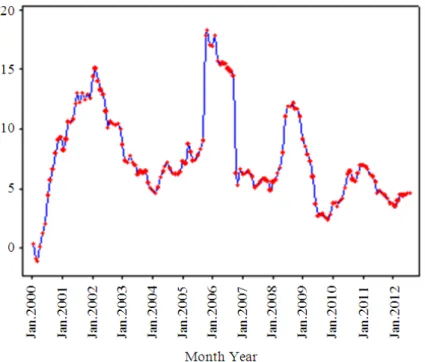
Figure 1 depicts the time series plot of the inflation series. From the figure, it is known that during the period Januari 2000 to Agustus 2012 the inflation in Indonesia has a regular trend on certain period, such as on February 2000 to February 2002 shows increasing trend, from March 2002 to February 2004 tends to decrease and different pattern observed for other periods.

Having applied nonlinearity test to the series above, it comes up with the conclusion that the inflation moves nonlinearl. Moreover, testing for long memory has also been applied to the series and it is obtained that the series has characteristic of being long memory process by introducing certain degree of fractional integration. Hence, the Indonesian inflation is a candidate of spurious long memory process. Furthermore, forecast combination will be conducted as a method to generate the forecast instead of selecting the best model. In fact, the best model is selected based on minimum average of the error and none of the model consistently generates best forecast in all periods. Prior to applying the forecast combination, the forecasts for 1 month ahead, 6 months ahead and 12 months ahead will be generated from long memory model and nonlinear models (Markov Switching and LSTAR).

3.1. Forecasting with ARFIMA

The first stage of ARFIMA model building is identification of some possible ARFIMA models with different order combinations. Furthermore, the best model will be selected to generate te forecast by considering the criterias of having small AIC, all parameters are significant and the residual of the model satisfies the assumptions of being white noise and normally distributed. Among the combinations, there are several candidates of ARFIMA models having small AIC as shown in Table 1.

Based on the table, it is known that the the smallest AIC is produced by ARFIMA (3,d,1). However, among

those models, ARFIMA (1,d,0) is the only model which satisfies the assumption required for the residuals of the model. Therefore, the forecast for three defined lead times will be generated by ARFIMA (1,d,0). The model has characteristic of stationary long memory process with the order of fractional difference of 0.261.

3.2. Forecasting with Markov Switching and

LSTAR

Similar to the forecasting using ARFIMA, the Markov Switching model is selected by considering the minimum AIC as well as the residual assumptions. The smallest AIC of the Markov Switching model is AR(1) where the residual satiisfies the required assumptions. The modeling process is done by estimating the transition matrix of the series. This research uses two regimes yielding on the following transition matrix:

0.902 0.990 0.098 0.010

P= 

 

Another nonlinear model used to forecast the inflation Logistic Smooth Transition Autoregressive (LSTAR). It is assumed that the delay equals to two and the series transit in two regimes. Similar modeling steps with ARFIMA and Markov Switching have been carried out, however best model which satisfies the assumption of normally distributed residual cannot be obtained. As the idea of the forecast is to minimize the forecast error, the best model is selected under the condition of minimum AIC and white noise. In this case, the LSTAR (1) is the candidate of the best model.

3.3. Forecast Combination

Fig. 1. Time series plot of Indonesian Inflation from 2000 to 2010 Table 1. Comparison of several ARFIMA models

Model AIC

ARFIMA (3,d,1) 71.337

ARFIMA (2,d,3) 73.154

ARFIMA (3,d,2) 73.402

ARFIMA (3,d,3) 74.739

ARFIMA (2,d,1) 75.660

ARFIMA (1,d,0) 81.986

3.4. Forecast Combination Using Balance Weight

As described in the previous section, the balace weight assigns the same weight to the forecast. Since we have three models to be combined, the weight will be 1/3 or it is a simple averaging. The variance of the forecast as the result of combination is given as:

2 2

, 1

ˆ

ˆ (ˆ ˆ )

K

t k t t k

k

W y y

σ

=

=

∑

Where: 2 ˆ_t

σ = Varians of the combined forecast on time t

ˆ_k

w = The weight

ˆ_t

y = The forecast on time

t and yˆt k, = The forecast form k-th single model on period t

The result of combination between ARFIMA, Markov Switching and LSTAR for Indonesian inflation forecast is presented in the table below. In this case, the inflation series is assumed to be normally distributed so that the estimated parameters are parameters of normal distribution used to calculate the interval forecast i.e., µ and σ2

.

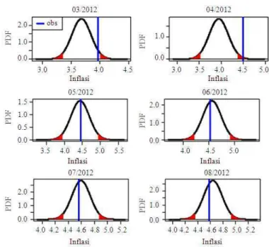
The interval is used to assess the forecast performance i.e., whether the forecast is capable to capture the observation or not. A good forecast will capture the observation with small interval widht. In order to clearly assess the performance of the forecast interval, the following Fig. 2 depicted plots of the forecasts and its corresponding observations. Only six last periods are presented as an illustration.

Fig. 2. PDF of forecast combination using balance weight for lead 12

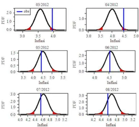
Fig. 4. PDF of forecast combination using balance weight for lead 1

3.5. Forecast Combination using Inverse Mean

Square Prediction Error (MSPE) Weight

The concept of estimating the weight using this method has been discussed in subsection 2.3.1. If the MSPE yields on small value on the m period of the forecast, thus the model is sufficiently acurate to forecast the observation and hence the weight is larger.

From Fig. 4, we can see that the MSPE forecast performs good by being able to capture the observation. The illustration about the forecast on 6 and 12 months ahead are skipped for the sake of simplicity. The comparison of the forecasting results for the whole period using m = 6 can be seen in Fig. 5. The result for m = 9 and m = 12 are omitted for the sake of space.

3.6. Forecast Combination Using Bayesian

Model Averaging (BMA)

In general, forecast combination using simple model averaging does not yield on reliable forecast for forecasting inflation either for lead 1, lead 6 or lead 12. It is expected that combination using Bayesian Model Averaging will improve the forecast reliability. Similar to MSPE, calibration using BMA requires the use of

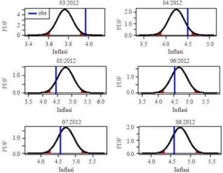
training window m. Figure 6 below performs the forecast performance only for several selected months.

Based on Fig. 7, using m = 6 we obtained 5 observations can be captured by the interval, meaning 88,46% observations lies with in interval of BMA forecast. Moreover, the interval is reliable enough with proper widht. This shows that the BMA performs good for lead 1 forecast especially using m = 6. Interval forecast for lead 6 and 12 are not as good as lead 1. In particular for m = 12 yields on very poor performance.

3.7. Comparison of the Forecast Accuracy of the

Combined Forecasts

This section performs comparison of the forecast accuracy using MSE and MAPE criterias. These two criterias assess the forecast performance deterministically. Table 2 summarizes the values.

Fig. 5. Plots of observations and forecast interval generated as the result of forecast combination using MSPE weight for lead 1, lead 6 and lead 12 with respectively

Fig. 7. Plots of observations and forecast interval generated as the result of forecast combination using BMA for lead 1, lead 6 and lead 12 with respectively

Table 2. MSE and MAPE comparison among three combination methods

Model averaging Lead-1 Lead-6 Lead-12

--- --- --- ---

Balance weight MSE MAPE MSE MAPE MSE MAPE

0.293 8.385 3.282 32.539 10.364 68.223 MSPE weight m = 6 0.202 6.584 2.941 30.425 6.998 54.024

m = 9 0.152 5.903 3.398 34.099 9.816 69.719

m = 12 0.135 5.641 4.025 40.009 12.762 83.565 BMA weight m = 6 0.185 6.783 4.539 38.325 10.685 70.585

m = 9 0.133 5.788 5.080 42.292 9.610 73.389

m = 12 0.169 7.201 5.989 50.464 15.881 90.680 Note: Minimum MSE: Minimum MAPE

Table 3. CRPS comparison among three combination methods

Method Mean CRPS

--- ---

Balance weight Lead-1 Lead-6 Lead-12

0.334 1.234 2.161

MSPE weight m = 6 0.271 1.147 1.731

m = 9 0.235 1.276 2.195

m = 12 0.216 1.503 2.614

BMA weight m = 6 0.250 1.599 2.838

m = 9 0.203 1.609 2.880

m = 12 0.238 1.830 3.521

MSE and MAPE assess the bias of the forecast only, without taking account into the width of the forecast interval. In order to assess both accuracy and resolution of the forecast, the Continuous Ranked Probability Score (CRPS) is used. The idea of the CRPS is to calculate the difference between CDF of the combination result with CDF of the observed inflation data. In this case, smaller CRPS shows better forecast reliability. Table 3 performs the mean CRPS over the whole forecast periods.

The CRPS shows that BMA with lead time of 9 yield on best forecast for lead 1, while MSPE outperforms BMA and balance weight for forecast on lead 6 and 12. General conclusion whether the forecast combination will always outperform the single model can be done by simulation study, which is the subject of the future research.

4. CONCLUSION

This research applies three different forecast combination approaches for forecasting Indonesian inflation. It has been proven that the Indonesian inflation can be modeled by long memory model as well as nonlinear models. However, it is unclear whether the long memory is true or spurious. The results of the analysis shows that the forecast combination can be a good approach for solving the confusion problem between these two competing processes. In term of the forecast accuracy, model combination outperforms the single model although the error is not significantly different. However, in the reality we never know which single model will generate the best forecast for forecasting the future inflation. Forecasting using forecast combination solve the problem by utilysing all information about the forecasts generated by all models. Among the three combination approach, BMA performs best for 1 ahead forecast, while MSPE perfors good for long lead time forecast.

5. REFERENCES

Beran, J., 1994. Statistics for Long-Memory Processes. 1st Edn., CRC Press, ISBN-10: 0412049015. pp: 315.

Drought, S. and C. McDonald, 2011. Forecasting house price inflation: A model combination approach. Discussion.

Geweke, J. and S. Porter-Hudak, 1983. The estimation and application of long memory time series models. J. Time Series Anal., 4: 221-237. DOI: 10.1111/j.1467-9892.1983.tb00371.x

Hamilton, J.D., 1989. A new approach to the economic analysis of nonstationary time series and the business cycle. Econometrica, 57: 357-384.

Hibon, M. and T. Evgeniou, 2005. To combine or not to combine: Selecting among forecasts and their combinations. Int. J. Forecast., 21: 15-24.

Hurvich, C.M., R. Deo and J. Brodsky, 1998. The mean squared error of geweke and porter-hudak’s estimator of the memory parameter of a long-memory time series. J. Time Series Anal., 19: 19-46. DOI: 10.1111/1467-9892.00075

Kuswanto, H., 2012. Artificial ensemble forecast: A new perspective of weather forecast in Indonesia. Proceedings of the International Conference on Mathematics and its Applications, Jul. 12-15, ITS Community.

Kuswanto, H., S. P. Irhamah and I. Koesniawanto, 2012. Bias Comparison on memory parameter of skip sampled long memory and exponentially smooth transition autoregressive process. Int. J. Applied Math. Stat.

Kuswanto, H., 2011. A new test against spurious long memory using temporal aggregation. J. Stat. Comput. Simul., 81: 1297-1311.

Kuswanto, H. and P. Sibbertsen, 2007. Can we distinguish between common nonlinear time series and long memory? Leibniz Hannover University, Germany.

Lobato, I.N. and N.E. Savin, 1998. Real and spurious long-memory properties of stock-market data. J. Bus. Econom. Stat., 16: 261-268.

Ohanissian, A., J.R. Russell and R.S. Tsay, 2008. True or spurious long memory? A New Test. J. Bus.

Econom. Stat., 26: 161-175. DOI:

10.1198/073500107000000340

Ravazzolo, F., 2007. Predictive Gains from Forecast Combinations Using Time Varying Model Weights. In: Forecasting Financial Time Series Using Model, Dalam F. Ravazzolo, Eds., Rotterdarm: Erasmus Universiteit Rotterdarm, pp: 19-56.

Raftery, A.E., T. Gneiting, F. Balabdaoul and M. dan Polakowski, 2005. Using bayesian model averaging to calibrate forecast ensembles. Am. Meteorogical

Society, 133: 1155-1174. DOI:

10.1175/MWR2906.1

Timmermann, A., 2006. Forecast Combinations. In: Handbook of Economic Forecasting, Elliot, G., C.W.J. Granger and A. Timmermann (Eds.), Elsevier, Amsterdam,ISBN-10: 0080460674, pp: 10-70. Wang, H. and S. Ma, 2008. The cytokine storm and

factors determining the sequence and severity of organ dysfunction in multiple organ dysfunction syndrome. Am. J. Emerg. Med., 26: 711-5. DOI: 10.1016/j.ajem.2007.10.031

Vrugt, J.A., C.G. Diks and M.P. dan Clark, 2008. Ensemble Bayesian model averaging using Markov Chain Monte Carlo Sampling. Environ. Fluid Mech., 8: 579-595. DOI: 10.1007/s10652-008-9106-3 Zivot, E. and D.J. Wang, 2006. Modelling Financial