Business cycle development in Czech and Slovak economies

BUSINESS CYCLE DEVELOPMENT

IN CZECH AND SLOVAK ECONOMIES

J. POMĚNKOVÁ

S. KAPOUNEK

Abstract:

Key words:

Department of Finance, Mendel University Brno.

1. Introduction

The process of European integration is often discussed by many politicians and academicians, almost only from the benefits and costs analysis point of view. Many empirical and theoretical studies quote the OCA theory properties. The theoretical foundations of currency union have been developed by Mundell (1961) to which many other authors subsequently contributed. The similarity of business cycles is the most important feature of the OCA, because if business cycles are synchronized, the costs of single monetary policy implementation are minimized.

There are many methods of business cycles synchronization measuring. Mostly

concordance index (Harding and Pagan, 2006).

Various studies have looked at the business cycle synchronization problem with different conclusions. These differences can be related to differences in the used variables, methods of business cycles estimation and synchronization measuring as well. The authors of this article deal with an alternate way to describe and measure synchronization of business cycles. The methodological approach focuses on different waves and different periods in the same business cycle.

The empirical part of the paper analyses Czech and Slovak economies. Czech Republic and Slovakia had experienced almost 75 years of common economic development. After disunion in 1992 both countries beat their own paths to the EU membership and later to the European Monetary Union. Both countries used their own strategies and also their own mix of macroeconomic policies, as they saw different sets of priorities and macroeconomic challenges. In spite of different policy strategy, after 1992 there are expected many similarities in the business cycle movements, especially in the waves and their periods.

2. Objectives

The business cycle estimations are related to the economic activity movements’ definition. Dornbusch (1984,

pp.λě describes business cycles as “more

or less regular pattern of expansion (recovery) and contraction (recession) in economic activity around the path of trend

growth.” In that event mathematical and statistical approach is used to identify business cycle movements. Especially, filter techniques are applied to estimate trend growth in the economic activity.

Many current empirical studies refer to an output gap – the distance between potential output and current GDP. The concept of output gap is very popular for its application from the economic policy stabilization function point of view. When the output gap is negative, the actual GDP is below its potential level and production factors are not being used intensively. In that case, monetary of fiscal expansionary policy is needed. The weakness of the output gap concept lies in a potential output estimation which is frequently based on the production function analysis. As the post-transformation economies are specified with many structural changes and insufficient number of observations, fluctuations of output around its trend level are often used.

The authors of this paper apply several mathematical statistic methodological approaches to identify business cycles, especially the first order differences (FOD), the auto-regression process (AR), the polynomial or linear regression (LF) and the Hodrick-Prescott filter (HP filter). Consequently, they abstract from the output gap approach and their business cycles estimation is based on the cyclical movements around the long-term trend in the economic activity.

price flexibility (Zarnowitz, 1992, pp.77-124). “Because output movements

are not regular, modern macroeconomics has generally turned away from attempts to interpret fluctuations as combinations of deterministic cycles of different lengths; efforts to discern regular Kitchin (3-year), Juglar (10-year), Kuznets (20-year), and Kondratiev (50-year) cycles have been

largely abandoned as unproductive.

(Romer, 2006, pp.175-176) There are as many theoretical approaches in contemporary literature as explanations for the existence of cyclical economic activity fluctuation around the long-term trend. Their simple explanation of the impact of one or several factors or shocks on the economic activity under mutual interaction and ceteris paribus conditions is very attractive and illustrative but rather imperfect when using empiric analyses. The cyclical fluctuation of economic activity actually aggregates many of identified or yet unidentified influences, while the expectations of economic entities and information availability on the market play an equally important role. (Kapounek, 2009)

Another problem in identifying the cyclical movements in economic activity is an indicator selection. A frequent indicator of economic activity is the gross domestic or national product. The main GDP limitations are exclusive of non-market transactions, underground economy existence, purchasing power of money variety in different proportion for different

goods and actual sale prices measurement (GDP does not capture the economic surplus between the price paid and subjective value received). For this article’s purposes, an Austrian economist’s critique is very important. Frank Shostak states that “The GDP framework cannot

tell us whether final goods and services that were produced during a particular period of time are a reflection of real wealth expansion, or a reflection of capital

consumption.” (Shostak, 2001) Very problematic is the key sector – government. If the government spends more, even if inefficiently, output goes up. Changes in the society and economy may have heightened this problem because the share of government output in GDP is increasing. Van den Bergh (2008) summarizes: “GDP really represents an

estimate of the costs instead of the benefits of all market-related economic activities in a country. In addition, GDP does not capture all social costs as it omits external

costs.” There are many other alternate indicators how to measure economic activity: index of industrial production, human development index, private product remaining etc.

Table 1 shows many similarities between the Slovak and Czech business cycle components. The major share of GDP comprises the consumption of households. Investments (gross capital formation) follow with 30 and 28%. The consumption expenditure of general government ranks the third position.

Percentage share of output components Table 1

Component of GDP Czech Republic Slovakia

Final consumption expenditure 72,42% 74,81%

Final consumption expenditure of households 51,10% 54,48% Final consumption expenditure of general government 20,74% 19,49%

Gross capital formation 30,00% 28,08%

Changes in inventories -1,85% 0,39%

Net exports -2,60% -2,56%

Exports of goods and services 73,35% 74,73%

The business cycle estimation in this article is based on the aggregate economic activity, represented by real GDP. The authors assume that the main problem of GDP is its aggregate character. The aggregate character of the GDP indicator, not its components provide all needed information about the economic system. Therefore, several periods are identified in the selected business cycles so as to be compared to one another.

2.1. Material and Methods

Standard theory of Burns and Mitchel (1946) business cycle is used. There are two approaches to business cycles. The first one is called the classical business cycle and is based on fluctuation in the level. The second one is known as the growth (deviation) cycle and is based on fluctuation around a trend.

If the models are designed to characterize the cyclical behavior, the trends are eliminated prior to the analysis. It is often useful to build a model where both trend and cyclical behavior are in the model and eliminate the trend from the model and from actual data in parallel fashion. The aim of such studies is to determine whether models capable of capturing salient features of economic growth can also account for observed patterns of business cycle activity. The specification of the model is subject to the constraint that it must successfully characterize the trend behavior. Having satisfied the constraint, trends are appropriately eliminated and the analysis proceeds with investigation of cyclical behavior. The isolation of cycles is closely related to the trends removal. Indeed, for a time series exhibiting cyclical deviations about a trend, the identification of the trend automatically serves to identifying the cyclical deviations as well. Notice that the removal of the trend will leave such fluctuation intact and their presence can

have a detrimental impact on inferences involving business cycle behavior.

Economic activity in this paper is measured by absolute values of GDP (yt)

transformed into the natural logarithms and denoted as Yt=ln(yt). For analysis of

business cycle additive decomposition method the form

Yt = gt + ct, i=1,...,n (1)

is used. The set of chosen de-trending methods is the following: the first order difference (FOD), random walk with/without a constant (ARc, AR), de-trending using a regression (LF, linear and quadratic trend) and Hodrick – Prescott filter (HP filter). Resultant deterministic models, quadratic one and AR (with or without a constant) were chosen according to the standard statistical techniques for quality evaluation. The wide range of de-trending methods is chosen with the aim of making results more robust. We are not

discussing whether these methods are “the best” for trend removing as well as which

one is more or less suitable and why. We just overview some of the commonly used methods as the result of other studies, for example Canova (1998, 1999), Baxter and King (1999) or Mills (2003) and search for statistically significant periods.

The procedure of HP filter was first introduced by Hodrick and Prescott in 1980 in the context of estimating business cycles. The HP filter decomposes Yt

(macroeconomic time series) into a nonstationary trend gt (growth component)

and a stationary residual component ct

(cyclical component)

Yt =gt + ct, t=1,...,n,

gt and ct are unobservable. The measure

of the gt path smoothness is the sum of the

squares of its second difference. The application of the HP filter involves minimizing the variance of the cyclical component ct subject to a penalty for the

 









 





min

1

2

1 1 1

2

1





      n t n

t t t t t

t t

gtT_t Y g  g g g g

(2)

where ct = Yt -gt . The parameter  is a

positive number which penalizes variability in the growth component series. Let lambda represents the weight. In many papers, a recommended lambda value for quarterly data is =1600 Ahumada, Garegnani (1990), Guy, St-Amant (1997), Hodrick-Prescott (1980) and others. In our study this value will be also used.

For periodicity analysis in the time series following harmonic analysis was used. After removing trend Tt, residuals were

obtained, i.e.

. ,..., 1

,t n

T Y

e_t  _t  _t 

For the analysis of random sequence in the form



 /2

1 ,..., 1 , )) sin( ) cos( ( n j t j j j j

t a t b t t n

e    

, (3)

where , aj, bj and ωj Ě0 < ωj  ) are

unknown parameters, et is a stationary

process, the periodogram is usually used.

In the points ω1,..., ωr the periodogram

constructed for given sequence of realization has relatively big values, and thus makes it possible to find estimates of

the parameters ω1,..., ωr including the value

r (the corresponding statistical procedure is

called the Fishers test of periodicity and is discussed later in the text). Coefficients aj,

bj are estimated using the ordinary least

squares method (OLS) in a standard way. The symbols aj, resp. bj, represent

regression parameters for the j-th smoothing sinusoida, resp. cosinusoida, and for its calculation holds the following formula derived on the basis of OLS

2 / ,..., 1 ), cos( 2 ), sin(

2 1 1

n j t e n b t e n a j n t t j j n t t

j 





 





. (4)

Next, variability corresponding to the j -th smoo-thing sinusoida and cosinusoida is calculated according to the formula

)

(

2

/

1

var



a



b

Testing the statistical significance of all possible periods and connected theoretical variance is done by the Fisher test ĚAnd l, 1976). As mentioned above, it is suitable to use some stationary tests; therefore we propose an augmented Dickey-Fuller (ADF) test (Wooldridge, 2003). 

3. Results and Discussion

Economic activity in this paper is measured by the values of Gross Domestic

Product (GDP) in the Czech Republic 1996/Q1 – 2008/Q3 and Slovakia 1993/Q1

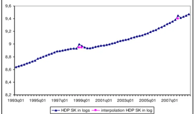
– 2008/Q3 in quarterly values. Input values of GDP are transformed into the natural logarithms and denoted as Yt (Figures 1, 2).

In the case of Slovakia, the input data situation with two jump phenomena in 1998/Q4 and 2007/Q4 arise. After each situation, GDP level returned to its long-run trend.

rate depreciation. After that, the government decreased fiscal expenditures. These changes contributed to the movements in the economic activity during the year 1998 and 1999. The second identified movement in the year 2007 was caused by a shock increase in consumption before the significant consumption taxes increase from the year 2008. Exactly, the stock of goods (not the real consumption) under the consumption taxes increased at the end of the year 2007.

Because both acts can be taken as short-term political shocks without important impact on the long-run trend behaving, the authors decided to interpolate three measurements, namely 1998/Q4, 1999/Q1

and 2007/Q4, by MA process with the length of 9. If it were the reverse, de-trending methods would indicate moments 1998/Q4, 2007/Q4 as structural breaks and the obtained results would have an impact on periodicity analysis.

The empirical analysis was done in the following steps: (i) testing stationarity of input values, (ii) de-trending using chosen method (FOD, AR, LF - polynomial or linear regression, HP filter) with the aim to obtain residuals, (iii) consequently, testing stationarity for residuals, (iv) application of harmonic analysis for identifying possible types of cycles in all given residuals.

12,9 13 13,1 13,2 13,3 13,4 13,5 13,6

1996q01 1998q01 2000q01 2002q01 2004q01 2006q01 2008q01

Fig. 1. GDP (natural logarithm values) for the Czech Republic 1996/Q1 – 2008/Q3

8,2 8,4 8,6 8,8 9 9,2 9,4 9,6

1993q01 1995q01 1997q01 1999q01 2001q01 2003q01 2005q01 2007q01 HDP SK in logs interpolation HDP SK in log

Fig. 2. GDP (natural logarithm values) for Slovakia 1993/Q1 – 2008/Q3

At first, the stationary test of input values was done. According to the ADF test the logarithmic values of Czech Republic GDP are trend (linear) stationary on 5%

or quadratic de-trending will be statistically valid. Despite this fact we are going to consider the FOD de-trending method usually suitable for difference stationary process (Wooldridge, 2003).

The chosen methods for de-trending were the first order difference (FOD, e1),

autoregression with/without a constant (AR, e2;ARc, e3), linear and quadratic time

trend (LF; e4) and Hodrick – Prescott filter

(HP filter, e5). Tables 2, 3 below describe

OLS estimates of some models for both countries. In the case of deterministic models the quadratic regression gives better results than the linear regression,

thus in the next analysis this type of regression is used. For AR process OLS estimated with and without a constant are significant. Hence, both cases were involved in the analysis of periods. Hodrick – Prescott filter is calculated for

smoothing the parameter = 1600 Ěe5).

Before applying the harmonic analysis, the residuals obtained by application of de-trending methods are tested for zero mean stationarity (ADF1). Table 4 shows the results. The notation "name of detrending method, corresponding residuals" is used, for example "FOD, e1".

Estimates of some chosen models for the Czech Republic Table 2

Parameters

estimate SE t-value F-test p-value Radj

2 _n

Quadratic regression 4609,24 1,4·10-55 0,9946 51 const. 13,1757 0,0042 4·10-129

t -0,0023 0,0004 2,1·10-7 t2 0,0002 7·10-6 2,5·10-32

AR const 4280,1 1,7·10-72 0,9988 50

const. -0,4527 0,0665 1,4·10-8 Yt-1 1,0346 0,0050 1,7·10

-72

AR 2,3·108 4·10-162 0,9796 50

Yt-1 1,0006 6,6·10

-5 _3·10-165

Statistical significance at the 1% (***), 5% (**), 10% (*) Source: Own calculation

Estimates of some chosen models for the Slovakia Table 3

Parameters

estimate SE t-value F-test p-value Radj

2 _n

Linear regression 1683,34 0,0000 0,9639 64 konst. 8,6448 0,0105 821,8767 0,0000

t 0,0115 0,0003 41,0285 0,0000

AR const 59562,77 0,0000 0,9990 63

const. -0,0774 0,0373 -2,0732 0,0424 Yt-1 1,0101 0,0041 244,0549 0,0000

AR 1,01·108 0,0000 0,9839 63

Yt-1 1,0015 0,0001 10065,7550 0,0000

Results of ADF stationarity test for the Czech Republic (CZ) and Slovakia (SK) Table 4

FOD, e1 ARc, e2 AR, e3 LF, e4 HP1600, e5

CZ No Yes, *** Yes,** Yes, *** Yes, ***

Lag 3 3 2 2

SK Yes No No Yes, *** Yes, **

Lag 1 6 6

Statistical significance at the 1% (***), 5% (**), 10% (*) H0: non-stationarity of et, t-stat. > quantil, (No)

H1: stationarity of et, t-stat. < quantil, (Yes) Source: Own calculation

Figures 3 and 4 show residuals corresponding to the de-trending method employed and the country.

-0,03 -0,025 -0,02 -0,015 -0,01 -0,005 0 0,005 0,01 0,015 0,02 0,025

1996q01 1998q01 2000q01 2002q01 2004q01 2006q01 2008q01

FOD,e1 Arc,e2 AR,e3 LF,e4 HP1600,e5

Fig. 3. Corresponding residuals for the de-trending methods used for the Czech Republic 1996/Q1 – 2008/Q3

-0,08 -0,06 -0,04 -0,02 0 0,02 0,04 0,06 0,08 0,1

1993q01 1995q01 1997q01 1999q01 2001q01 2003q01 2005q01 2007q01

FOD,e1 Arc,e2 AR,e3 LF,e4 HP1600,e5

In the case of the Czech Republic the empirical analysis showed that the first order difference as well as random walk is not a suitable detrending technique. The FOD residuals are not stationary and are correlated with trend component (r = 0,75) (Canova, 1998). Random walk process has such statistics that random walk with a drift. Thus, in the Czech Republic data set, both methods produce inputs to the dating process of the classical cycle. In addition, despite satisfaction assumptions of UC method, it was decided not to recommend this method as detrending for the Czech Republic’s case. When comparing FOD and AR residuals’ shape and AR cons. the residuals’ shape can be seen

“eyemetrically” similar, especially in the

first half of the period. In the second half of the period the curve shape is more similar to the FOD residuals. Detrending using regression represented by quadratic trend, has acceptable statistics of quadratic regression estimate and is useful. In the case when =1600 for Hodrick-Prescott filter was considered, obtained residuals looked the same as linear filtering residuals. From this point of view both methods can be taken as giving the same cyclical fluctuation.

In the case of Slovakia the empirical analysis showed that the first order difference as well as the Hodrick-Prescott filter with =1600 can be used for detrending. Detrending using regression represented by linear trend is also useful, regression statistics are good (Table 3), but as it can be seen in Figure 4 the residuals after linear de-trending show greater

variance. It is because linear trend does not represent the data trend behaviour as for example with the Hodrick-Prescott filter. Random walk process with/without a drift is not useful, the obtained residuals are not stationary (Table 4).

In the following step application, the harmonic analysis for the identification of possible types of cycles is done. For the Czech Republic (the results are in Table IV) the residuals of linear filtering and Hodrick-Prescott filtering are used. For Slovakia (the results are in Table V) FOD, detrending using regression and Hodrick-Prescott filtering is used. The results of calculated periodicity and testing statistical significance are given in Table 4. Notice that the input values are quarterly, i.e. for example 50 periods is a 12.5 year-duration. In spite of the Romer (2006) critiques of regular periodicities in the business cycles, the authors identified regularities in different waves. According to periodicity, Schumpeter (1939) proposed the following group of cycles named by the scientist who identified their existence in time series. The shorter one is the Kitchin inventory cycles of 3-5 years. Then the Juglar fixed investment cycles of middle length, 7-11 years. And the longer one, the Kuznets infrastructural investment cycles of 12-25

years. The longest one, Kondratieff’s

Results of statistical significance of periods for the Czech Republic Table 5

periods 50 25 16,7 12,5 10 8,3 7,1

LF,e2 *** *** ***

HP1600,e5 *** *** *** *** ** *** ***

Statistical significance at 1% (***), 5% (**), 10% (*) Source: Own calculation

Results of statistical significance of periods for Slovakia Table 6

periods 63 31,5 21 15,8 12,6

FOD,e1 *** **

LF,e2 *** *** *** *** **

HP1600,e5 *** *** *** *

Statistical significance at 1% (***), 5% (**), 10% (*) Source: Own calculation

Comparison of duration of periods, the Czech Republic and Slovakia Table 7 very short short middle long Cycles duration (years) <3 3-5 7-11 12-25 The Czech Republic x x x x

Slovakia x x x

Statistical significance at 1% (***), 5% (**), 10% (*) Source: Own calculation

If we compare the results of both countries (Tables 5, 6, 7), we can see, in the Czech Republic, a statistically significant wide range of cycle duration – a long one as well as middle and short cycles. Even very short cycles of duration of approximately two years were identified. In comparison with this, Slovakia does not have very short cycles, but the remaining range of cycle duration is similar.

It is necessary to say that the success of dating growth cycles crucially depends on the quality of the approximation of the trend component.

4. Conclussion

The frequency analysis (harmonic analysis approach) identified different waves with different periods in the same business cycle. In spite of many similarities between the Czech and Slovak economies, the waves are of asymmetric character at different frequencies. This conclusion assumes that a common stabilization macroeconomic policy is not efficient.

Acknowledgements

The results introduced in the paper are supported by the research intent n. MSM

6215648λ04 with the title “The Czech

Economy in the Process of Integration and Globalisation, and the Development of Agricultural Sector and the Sector of Services under the New Conditions of the

Integrated European Market”.

References

1. And l, J.: Statistická analýza časových

řad. SNTL, Praha. 1976, p. 271. 2. Ahumada, H., Garegnani, M. L.:

Hodrick-Prescott Filter in practice. UNLP 1999.

3. Baxter, R., King, R. G.: Measuring Business Cycles: Approximate Band – Pass Filters for Economic Time Series. Review of Economic and Statistics, 1999, vol. 81, no. 4, pp. 575-593. 4. Burns, A. F., Mitchell, W. C.:

Measuring Business Cycles. New

York. 1946, National Bureau of Economic Research, p. 590.

5. Canova, F.: De-trending and business cycle facts. Journal of monetary Economic, 1998, vol. 41, pp. 533-540. 6. Canova, F.: Does De-trending Matter

for the Determination of the Reference Cycle and Selection of Turning Points?

The Economic Journal, 1999, Vol. 109, No. 452, pp. 126-150.

7. Croux, CH., Forni, M., Reichlin, L.: A

Measure of Comovement for Economic Variables: Theory and Empirics.

Centre for Economic Policy Research. Discussion Paper No. 2339. December 1999.

8. Darvas, Z., Szapáry, G.: Business Cycle Synchronization in the Enlarged EU. Centre for Economic Policy Research. Discussion Paper No. 5179. August, 2005.

9. Dornbusch, F.: Macroeconomics.

Third Edition. New York: 1984, McGraw-Hill Book Company, pp. 5-18.

10. Guay, A., St-Amant, P.: Do the

Hodrick-Prescott and Baxter-king

Filters Provide a Good Approximation of Business Cycles? Université a Québec á Montreál 1997, Working paper No. 53.

11. Harding, D., Pagan, A.:

Synchronization of cycles. Journal of Econometrics, 2006, Volume 132, Issue 1, pp. 59-79.

12. Hodrick, R. J., Prescott, E. C.: Post-war U.S.1980. Business Cycles: An Empirical Investigation, Mimeo, Carnegie-Mellon University, Pitsburgh. 1980, PA. p. 24.

13. Kapounek, S.: Estimation of the

Business Cycles - Selected

Methodological Problems of the

Hodrick-Prescott Filter Application.

Polish Journal of Environmental Studies, 2009 Nr. 6.

14. Koopman, S. J., Azevedo, J. V.:

Measuring Synchronisation and

Convergence of Business Cycles.

Tinbergen Institute Discussion Paper. Amsterdam. 2003.

15. Mill, T. C.: Modelling Trends and

Cycles in Economic Time Series.

16. Mundell, R.: A Theory of Optimum

Currency Areas. The American

Economic Review 51, 1961, pp. 657-665.

17. Romer, D.: Advanced Macroeconomics. Third Edition. New York. 2006, McGraw-Hill/Irwin Companies, p. 678. 18. Shostak, F.: What is up with the GDP?

Mises Daily [online]. Auburn: Ludwig von Mises Institute, August 2001 [cit. 2010-03-15]. Web pages < http://mises.org/daily/770>

19. Van Den Bergh, J. C. J. M.: The GDP

Paradox. Journal of Economic

Psychology, 2008, No 30. 2009.

pp. 117-135.

20. Wooldridge, J. M.: Introductory

Econometrics: A modern approach.

Ohio 2003, s. 863.

21. Zarnowitz, V.: Business Cycles,

Theory, History, Indicators and

Forecasting. Chicago 1992, The