Aggregate uncertainty, disappointment aversion and the business cycle

(1)

Funda¸c˜ao Get´ulio Vargas

Escola de P´os-Gradua¸c˜ao em Economia - EPGE

Aggregate Uncertainty, Disappointment Aversion and the

Business Cycle

Aluna: Júlia Fernandes Araújo da Fonseca Orientador: Marco Antonio César Bonomo

Co-orientador: Tiago Couto Berriel

Rio de Janeiro

(2)

Funda¸c˜ao Get´ulio Vargas

Escola de P´os-Gradua¸c˜ao em Economia - EPGE

Aggregate Uncertainty, Disappointment Aversion and the

Business Cycle

Disserta¸cão submetida à Escola de Pós-Gradua¸cão em Economia

da Funda¸cão Getúlio Vargas como requisito de obten¸cão do t´ıtulo de

Mestre em Economia

Aluna: J´ulia Fernandes Ara´ujo da Fonseca

Banca Examinadora:

Marco Antonio C´esar Bonomo (EPGE-FGV/RJ) Tiago Couto Berriel (EPGE-FGV/RJ)

Ricardo Dias de Oliveira Brito (Insper)

(3)

Ficha catalográfica elaborada pela Biblioteca Mario Henrique Simonsen/FGV

Fonseca, Júlia Fernandes Araújo da

Aggregate uncertainty, disappointment aversion and the business cycle / Júlia Fernandes Araújo da Fonseca. – 2013.

23 f.

Dissertação (mestrado) - Fundação Getulio Vargas, Escola de Pós-Graduação em Economia.

Orientador: Marco Antonio César Bonomo. Coorientador: Tiago Couto Berriel.

Inclui bibliografia.

1. Finanças. 2. Incerteza. 3. Risco (Economia). 4. Investimentos. 5. Modelos macroeconômicos. I. Bonomo, Marco Antônio Cesar. II. Berriel, Tiago Couto. III. Fundação Getulio Vargas. Escola de Pós-Graduação em Economia. IV. Título.

(4)

(5)

Abstract

We investigate the effect of aggregate uncertainty shocks in real variables. More specifi-cally, we introduce a shock in the volatility of productivity in an RBC model with long-run volatility risk and preferences that exhibit generalised disappointment aversion. We find that, when combined with a negative productivity shock, a volatility shock leads to fur-ther decline in real variables, such as output, consumption, hours worked and investment. For instance, out of the 2% decrease in output as a result of both shocks, we attribute 0.25% to the effect of an increase in volatility.

We also find that this effect is the same as the one obtained in a model with Epstein-Zin-Weil preferences, but higher than that of a model with expected utility. Moreover, GDA preferences yield superior asset pricing results, when compared to both Epstein-Zin-Weil preferences and expected utility.

(6)

1 Introduction

In this paper, we are concerned with the effect that an increase in uncertainty has on eco-nomic activity. Our motivation stems, in part, from empirical evidence that an increase in volatility has a negative effect on real variables such as output and hours worked, as in Bloom [2009].

To investigate this effect, we introduce in an otherwise standard RBC two assumptions: stochastic volatility (as Fernandez-Villaverde and Rubio-Ramirez [2010]) and preferences that exhibit generalized disappointment aversion (henceforth GDA). To the best of our knowledge, this is the first attempt to investigate the quantitative effects of these prefer-eces in a macroeconomic model.

Preferences that exhibit disappointment aversion were first introduced by Gul [1991] and later generalized by Routledge and Zin [2010]. GDA preferences overweight outcomes below a certain threshold, which is set as a fraction of the certainty equivalent of future utility. A particular case of GDA is disappointment aversion, when the threshold is set at the certainty equivalent. As we will see further on, both Epstein-Zin-Weil preferences and expected utility can also be seen as a particular case of GDA. We compare the results we obtain with GDA preferences with those implied by both of these particular cases. We find that, when in conjuction with a negative productivity shock, volatility shocks have real and quantitatively relevant effects. However, a volatility shock alone appears to have little impact on economic activity in this model.

Also, the effect of a volatility shock in the baseline model is the same as in a model with Epstein-Zin-Weil preferences, although the asset pricing implications differ. This is most likely due to the fact that, under our baseline calibration, the agent is disappointed in less than 1% of the state space. We would have liked to induce higher levels of disappointment, but were unable to obtain convergence for certain parametric regions.

Regarding the model with expected utility, we find that the impact of a volatility shock is smaller than in the baseline model and in that with Epstein-Zin-Weil preferences. Since the agent with expected utility atributes higher value to consumption smoothing, labor, investment and consumption are less impacted by the shock.

(8)

in the volatility of interest rates at which small open economies borrow impact economic activity in a small open economy business cycle model with stochastic volatility in the process for real interest rates. They find that an increase in the volatility of real interest rates leads to a decrease in output, consumption, investment and hours worked. We depart from both these contributions, as we obtain our results in general equilibrium in a simple RBC that is calibrated to match observations of a developed economy.

Our paper is related to the literature on time-varying volatility in macroeconomics, which considers models with heteroskedasticy and aims to determine to what extent, if any, variations in volatility affect economic activity. Justiniano and Primiceri [2008] and Fernandez-Villaverde and Rubio-Ramirez [2007] estimate DSGE models with het-eroskedastic shocks driving the dynamics of the economy to account for the “Great Mod-eration”. Christiano et al. [2010] shows that shocks to the volatility of individual firms’ productivity have a considerable effect on the business cycle. Fernandez-Villaverde et al. [2012] assesses the economic impact of the increase in aggregate uncertainty regarding fiscal policy.

Also, since the work of Bansal and Yaron [2004], a large literature has been developed around the concept of long-run risks - persistent shocks to growth rates and uncertainty. Models of long-run risks have been applied to explain a variety of asset market puzzles, such as the high equity premium and the return premium on value stocks. Bonomo et al. [2011], incorporates preferences that display GDA in an asset pricing model with long-run volatility risk. Nakamura et al. [2012] quantifies the importance of long-long-run risks and identifies sizable and persistent world growth-rate shocks. They also estimate uncertainty shocks to be considerably more persistent than growth-rate shocks. Bansal et al. [2012] shows that volatility risk affects consumption and that ignoring volatility news leads to miss-specification on the stochastic discount factor. This paper is also related to this literature, as we consider a model with a form of long-run volatility risk.

2 The Model

(9)

2.1 Household

There is an infinite lived representative household with preferences over consumption,ct,

and leisure, 1−lt, that exhibit GDA. We represent the recursive intertemporal utility

functional by:

Ut=

     n

(1−β)(cυ

t −kl1t−ν)

1−1

ψ +β[R

t(Ut+1)]1−

1

ψ

o 1 1₋1

ψ if ψ 6= 1

(cυ

t −klt1−ν)1−β[Rt(Ut+1)]β if ψ = 1

, (1)

where β is the time preference discount factor, ψ is elasticity of intertemporal substi-tution, and Rt(Ut+1) is the certainty equivalent of future utilility conditional on time t

information. In the case of GDA preferences, the certainty equivalent is implicitly defined by:

R1−γ

1−γ =

Z

(−∞,∞)

U1−γ

1−γdF(U)−

1 a −1

Z

(−∞,κR)

κR1−γ

1−γ − U1−γ

1−γ

dF(U),

where 0< a ≤1 and 0< κ ≤1. When a < 1, outcomes that are lower than κR receive an extra (negative) weight, decreasing the certainty equivalent. Hence, a can be seen as a measure of disappointment aversion, whileκ is the fraction of the certainty equivalent

R that determines the threshold below which outcomes are considered disappointing. Note that, when a = 1, R becomes the certainty equivalent corresponding to expected utility and Ut represents Epstein-Zin-Weil preferences (Epstein and Zin [1989]; Weil

[1990]). Also, when a = 1 and ψ = 1/γ, these preferences collapse into the expected utility framework. Hence, both Epstein-Zin-Weil preferences and expected utility are particular cases of GDA preferences.

The household’s budget constraint is given by:

ct+it+

bt+1

R_tf =wtlt+rtkt+bt, (2)

where it is investment, Rft is the risk-free gross interest rate, bt is the holding of an

uncontingent bond that pays one unit of the consumption good at time t+ 1, lt is labor,

rt is the rental rate of capital and kt is capital.

(10)

kt+1 = (1−δ)kt+it, (3)

where δ is the depreciation rate.

2.2 Firm

The final good is produced by a competitive firm with Cobb-Douglas technology:

yt =ezt−

1 2V[zt]kζ

tl1t−ζ, (4)

where zt is the productivity level and evolves as:

zt=λzt−1+eσtεt, εt∼ N(0,1). (5)

Since we would like to isolate the effect of a change in the volatility of productivity, we don’t define the Solow residual as ezt_{. That is because, given} _σ

t, ezt has log-normal

distribution. Hence, an increase in σt would also increase the mean of productivity,

eE_[_z_t]+1

2V[zt]. Hence, the Solow residual is defined as ezt− 1

2V[zt], where V[z_t] is the variance

of zt.

Note that we are incorporating time-varying volatility in the process for productivity, in order to assess the effect of a shock to the volatility of productivity. In the literature, these changes in volatility are usually modeled in one of three ways: stochastic volatility, GARCH process or Markov switching regime.

We decide against the GARCH approach, as it would require that the inovation to the volatility of productivity be εt, which is the inovation to the level of productivity. That

means we would not be able to separate a volatility shock from a productivity shock. This problem is not present with either stochastic volatility or Markov switching and both would be suitable for our purpose. We opt for stochastic volatility, which is used in a large part this literature, such as Villaverde et al. [2011] and Fernandez-Villaverde et al. [2012].

(11)

σt= (1−ρ)¯σ+ρσt−1+ηωt, ωt∼ N(0,1). (6)

2.3 Equilibrium

Definition A competitive equilibrium is a sequence of allocations {ct, lt, it, yt}∞t=0 and

prices {wt, rt, Rft}∞t=0 such that:

1. Given prices{wt, rt, Rtf}∞t=0, the representative household maximizes utility (1)

sub-jected to budget constraint (2).

2. Given prices {wt, rt, Rft}∞t=0, the firm minimizes costs given production function (4)

3. Markets clear: the law of motion for capital (3) holds and yt =ct+it

4. Productivity follows equations (5) and (6)

3 Calibration and Solution

3.1 Calibration

We calibrate the model to match observations of the U.S. economy, following Bonomo et al. [2011] for certain parameters of GDA preferences.

We set ν, the parameter that governs labor supply, to 0.7576 and k = 1.4705, to get the representative household to work one third of its time in steady state and to ensure that the Frish elasticity of labor supply equals 1 in steady state. We set the elasticity of output to capital ζ = 0.3, so as to match the labor share of national income. The depreciation rateδ is set to 0.0196 to match the ratio of investment to output. Following Caldara et al. [2012], λ= 0.95, e¯σ _{= 0.007,} _ρ_{= 0.9 and} _η_{= 0.06.}

As in Caldara et al. [2012], we set the discount factor β = 0.991 to generate an anual interest rate of 3.6%. Following Bonomo et al. [2011], we set the elasticity of intertemporal substitutionψ = 1.5, the risk aversionγ = 2.5 and the disappointment aversion parameter a= 0.3.

(12)

that 0.99956, we were unable to achieve convergence at the level of 10−6_.

The values for the parameters are summarized in Table 1: Table 1: Calibration

Parameter Value

β 0.991

ψ 1.5

γ 2.5

υ 0.5

ν 0.7576

k 1.4705

ζ 0.3

δ 0.0196

λ 0.95

¯

σ 0.007

ρ 0.9

η 0.06

a 0.3

κ 0.99956

3.2 Solution method

Regarding the solution method, the fact that GDA preferences have non-differentiabilities and kinks prevented us from using either perturbation methods or Chebyshev polyno-mials. Hence, we solve the model through value function iteration. Since both welfare theorems hold, we can refer to the value function representation of the social planner’s problem:

V(kt, zt, σt) = max ct,lt,kt+1

n

(1−β)(cυ_t −kl_t1−ν)1−ψ1 +β[R

t(V(kt+1, zt+1, σt+1))]1−

1

ψ

o 1 1−_ψ1

s.t. ct+kt+1 =ezt−

1 2V[zt]kζ

tlt1−ζ+ (1−δ)kt

zt =λzt−1+eσtεt, εt ∼ N(0,1)

σt= (1−ρ)¯σ+ρσt−1+ηωt, ωt∼ N(0,1)

(13)

1. Set i= 0, V0_(k

t, zt, σt) = (eztcss)u−hl(1+ss ν) and R0(kt, zt, σt) = E[(V0)1−γ], where

css and lss are the non-stochastic steady state values for consumption and labor,

respectively.

2. Obtain the certainty equivalent R in a secondary loop, which will be described next.

3. For every {kt, zt, σt}, compute the possible values ofV and find the maximum value

Vi+1 _and _ci+1

t , lti+1, kti+1+1 that produce this maximum value.

4. If dif f = max|Vi+1_|_V−i_|Vi| ≥10−6, set i=i+ 1 and go to step 2. Otherwise, stop.

The algorithm of the secondary loop, used to obtain the certainty equivalent, is: I Set j = 0 andRj ₌_Ri_.

II Set Rj+1 _{= (}R

(−∞,∞) (Vi₎1₋γ

1−γ dF(Vi)− a1 −1 R

(−∞,κRj₎(

κ(Rj₎1₋γ 1−γ

(Vi₎1₋γ

1−γ )dF(Vi))1/(1−γ)

III If max |Rj+1_|Rj−R_| j| ≥ Θdif f, set j =j + 1 and go to step II. Otherwise, stop and set

Ri ₌_Rj+1_{. In this exercise, we use Θ = 30.}

As in Caldara et al. [2012], we start by iterating on a small grid. After convergence, we increase the size of the grid and use the previous value function as an initial guess, using linear interpolation to atribute values to the new grid points. We work up to a state space with 375,000 (3000 points for capital, 25 for productivity and 5 for volatility). Also, to accelerate convergence even further, we: (i) update the value function for a subset of the state space and use linear interpolation to obtain the values for the remaining points and (ii) implement step 3 in a region around the solution of the previous iteration, ci

t, lit, kti+1.

4 Effect of an Increase in Aggregate Uncertainty

(14)

in the near future. Depending on the effect on labor, we could expect an increase or a decrease in investment.

To assess the effect of a volatility shock in this simple framework, we compute impulse response functions to a 2 standard deviation shock to σ, the log of the volatility of productivity. Also, we look at the IRFs of a combined volatility shock and negative productivity shock of the same magnitude, to see whether this interaction changes the impact uncertainty might have on economic activity.

4.1 Simulation method

Since we are interested in investigating the effect of an increase in volatility, we use as the starting point for our impulse response functions the stochastic steady state of the model.

Hence, after the initial shock, we draw from the standard normal distribution a sequence of realizations of the stochastic components (ε and ω) and simulate the trajectory of the economy for the remainder of the simulation period. We repeat this exercise 20000 times and define the IRFs as the average of all simulations, so that variables converge once again to the stochastic steady state. All IRFs are expressed as deviation from stochastic steady state.

4.2 Volatility shock

(15)

0 10 20 30 40 50 60 70 80 90 100

−2 0 2 4

x 10−5 c o n s u m p t i o n(c)

0 10 20 30 40 50 60 70 80 90 100 0

0.5 1

x 10−3 v o l a t i l i t y(σ)

0 10 20 30 40 50 60 70 80 90 100 0

2 4 6

x 10−4 c ap ital (k )

0 10 20 30 40 50 60 70 80 90 100

−2 0 2 4 6

x 10−6 lab or (l)

0 10 20 30 40 50 60 70 80 90 100

−2 0 2 4x 10

−5 _{i nv e stm e nt (i)}

0 10 20 30 40 50 60 70 80 90 100 0

2 4 6 8x 10

−5 _{ou tp u t (y )}

0 10 20 30 40 50 60 70 80 90 100

−3

−2

−1 0 1

x 10−5 p ro d u c tiv ity (z )

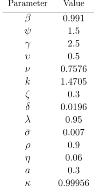
Figure 1: Impulse Response Functions to a volatility shock minus trajectory in the absence of shocks.

In Figure 1, it’s important to note that the scale of the effect for most variables is 10−5_{, which is the same scale of the movements in productivity. While the volatility of}

productivity remains high, we can see larger movements in productivity, which in turn seem to be causing other variables to oscillate as well.

It appears that a volatility shock alone has little impact on economic activity in this model.

4.3 Volatility shock and productivity shock combined

Next, we evaluate the impact of a volatility shock combined with a negative productivity shock, relative to a negative productivity shock alone.

(16)

0 10 20 30 40 50 60 70 80 90 100

−0.01

−0.005 0

c o n s u m p t i o n(c)

0 10 20 30 40 50 60 70 80 90 100

−5 0 5 10x 10

−4 _{v o l a t i l i t y}₍σ)

0 10 20 30 40 50 60 70 80 90 100

−0.15

−0.1

−0.05 0 0.05

c ap ital (k )

0 10 20 30 40 50 60 70 80 90 100

−4

−2 0 2

x 10−3 lab or (l)

0 10 20 30 40 50 60 70 80 90 100

−15

−10

−5 0 5

x 10−3 inv e stm e nt (i)

0 10 20 30 40 50 60 70 80 90 100

−0.03

−0.02

−0.01 0

ou tp u t (y )

0 10 20 30 40 50 60 70 80 90 100

−0.02

−0.01 0 0.01

p rod u c tiv ity (z )

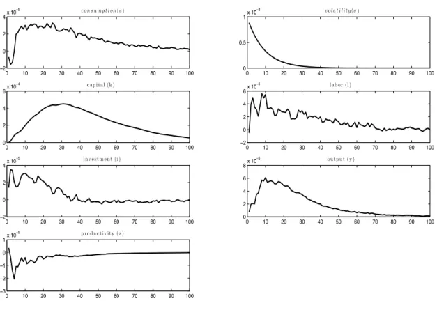
Figure 2: Impulse Response Functions to a negative productivity shock combined with a volatility shock in the model with GDA preferences expressed as deviation from stochastic steady state.

In the simulated stochastic steady state, the Solow residual is 0.996 and the standard deviation of productivity is 0.007. After the combined shock to both productivity and volatility, the Solow residual falls to 0.98 and the standard deviation rises to 0.008. As we can see, the combination of both shocks results in a decrease in consumption, hours worked, investment, capital and output. As we know, a negative productivity shock reduces the marginal product of labor, reducing the demand for labor and the amount of hours worked, and shifts the production function downward. As a result, output falls, the real interest rate rises and investment and consumption fall.

(17)

0 10 20 30 40 50 60 70 80 90 100

−1

−0.5 0

0 10 20 30 40 50 60 70 80 90 100 0

0.5 1

0 10 20 30 40 50 60 70 80 90 100

−0.015

−0.01

−0.005 0

c ap i tal (k )

0 10 20 30 40 50 60 70 80 90 100

−6

−4

−2 0x 10

−4 _{l ab or (l )}

0 10 20 30 40 50 60 70 80 90 100

−2

−1 0 1

x 10−3 inv e stm e nt (i )

0 10 20 30 40 50 60 70 80 90 100

−3

−2

−1 0

x 10−3 ou tp u t (y )

0 10 20 30 40 50 60 70 80 90 100

−2

−1.5

−1

−0.5 0x 10

−3 _{p ro d u c ti v i ty (z )}

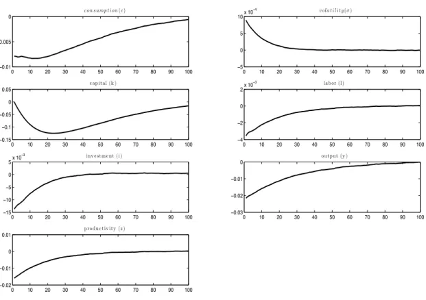
Figure 3: Impulse Response Functions to a negative productivity shock combined with a volatility shock minus Impulse Response Functions to a productivity shock alone.

The result is that the addition of a volatility shock intensifies the decrease in economic activity. In a state of the world in which productivity is low, high volatility of productivity induces the representative agent to work even less, since the probability of having higher productivity in the near future is high.

Also, low productivity means that the agent is poorer, which drives him to a more concave region of his utility function. In other words, in this low productivity state of the word, the agent values certainty even more, which strengthens his precautionary motive. This leads to a decrease in consumption and investment, which in turn causes output to fall even further.

(18)

4.4 Evaluating the results

We now briefly compare our results with other works in the literature of time-varying volatility and second moment shocks.

In Bloom [2009], in the aftermath of a shock to the volatility of business conditions, output falls 2% and employment falls 1.5%. So not only does this work obtain real effects to a volatility shock alone, this effect is considerably larger than the one we can attribute to the rise in volatility in our combined shock exercise. We can also emphasize, however, that we obtain our results in a general equilibrium framework without adjustment costs. Also, in Bloom [2009], a volatility shock consists of almost doubling volatility, on average. Another related work is Fernandez-Villaverde et al. [2011], which analyses how changes in the volatility of the real interest rate at which emerging economies borrow impact real economic activity. They calibrate the model to match observations of four different countries (Argentina, Ecuador, Venezuela and Brazil) and report the results of a volatility shock. The shock decreases output in 0.15% in Argentina, 0.1% in Ecuador, 0.007% in Venezuela and 0.006% in Brazil.

In this case, the impact of a volatility shock decreases with the standard deviation of the stochastic volatility. The standard deviation on the volatility of interest rates for Brazil in 0.28, whereas we set the standard deviation of the volatility of production as 0.06. Hence, it’s important to note that we obtain our results in a framework calibrated to match observations of a developed economy, in which the stochastic process is less volatile and, therefore, volatility shocks are smaller.

After this brief comparison, we can highlight that (i) not much has been done in this liter-ature in general equilibrium and calibrating to match observations of developed economies and (ii) empirical exercises aren’t focusing on the interaction between volatility shocks and negative productivity shocks, which seems like a natural channel for the effects of an increase in aggregate uncertainty in general equilibrium.

5 Epstein-Zin-Weil preferences and Expected Utility

(19)

to obtain Epstein-Zin-Weil preferences, we set a = 1 and, to collapse into the expected utility framework, we set a= 1 and ψ = 1/γ = 0.4.

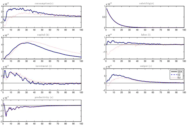
In Figure 4, we present the results of a volatility shock for all 3 models:

0 10 20 30 40 50 60 70 80 90 100

−4

−2 0 2 4

0 10 20 30 40 50 60 70 80 90 100 0

0.5 1

0 10 20 30 40 50 60 70 80 90 100 0

2 4 6

x 10−4 c ap i tal (k )

0 10 20 30 40 50 60 70 80 90 100

−2

−1 0 1

x 10−5 l ab or (l )

0 10 20 30 40 50 60 70 80 90 100

−2 0 2 4

x 10−5 inv e stm e nt (i )

0 10 20 30 40 50 60 70 80 90 100

−5 0 5 10

x 10−5 ou tp u t (y )

0 10 20 30 40 50 60 70 80 90 100

−3

−2

−1 0 1

x 10−5 p ro d u c ti v i ty (z )

GDA EZ EU

Figure 4: Impulse Response Functions to volatility shock minus trajectory without shocks: In the solid black line, we have the IRF for the model with GDA (a = 0.3), in the dashed line, the IRF for the

Epstein-Zin-Weil model (a = 1) and, in the dotted line, the IRF for the model with expected utility

(a= 1 andψ= 0.4).

(20)

0 10 20 30 40 50 60 70 80 90 100

−0.01

−0.005 0

c on s u m p t i on(c)

0 10 20 30 40 50 60 70 80 90 100

−5 0 5 10x 10

−4 _{v ol a t i l i t y}₍σ)

0 10 20 30 40 50 60 70 80 90 100

−0.15

−0.1

−0.05 0 0.05

c ap ital (k )

0 10 20 30 40 50 60 70 80 90 100

−4

−2 0 2x 10

−3 _{lab or (l)}

0 10 20 30 40 50 60 70 80 90 100

−15

−10

−5 0 5x 10

−3 _{inv e stm e nt (i)}

0 10 20 30 40 50 60 70 80 90 100

−0.03

−0.02

−0.01 0

ou tp u t (y )

0 10 20 30 40 50 60 70 80 90 100

−0.02

−0.01 0 0.01

p rod u c tiv ity (z )

GDA EZ EU

Figure 5: Impulse Response Functions to both shocks: In the solid line, we have the IRF for the model with GDA (a= 0.3), in the dashed line, the IRF for the Epstein-Zin-Weil model (a = 1) and, in the

dotted line, the IRF for the model with expected utility (a= 1 andψ= 0.4).

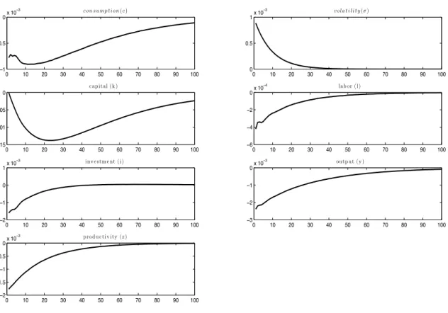
From Figure 5, we can see that, under our baseline calibration, the results obtained with Epstein-Zin-Weil preferences are the same as those implied by the model with generalized disappointment aversion. A possible explanation is the fact that, with κ = 0.99956, the representative agent is disappointed in less than 1% of the state space. Hence, it is possible that the disappointment aversion isn’t large enough to distinguish the agent’s choices from that of an agent with Epstein-Zin-Weil preferences when both are faced with a shock of this magnitude. As we will see further on, however, the asset pricing implications from both models differ.

We can also notice that effect of the shocks is higher in the models with Epstein-Zin-Weil preferences and GDA than in the model with expected utility. Since the elasticity of intertemporal substitution equals 0.4 in the expected utility model, the representative agent atributes greater value to consumption smoothing than an agent with ψ = 1.5. Hence, the decrease in labor, investment and consumption is smaller.

(21)

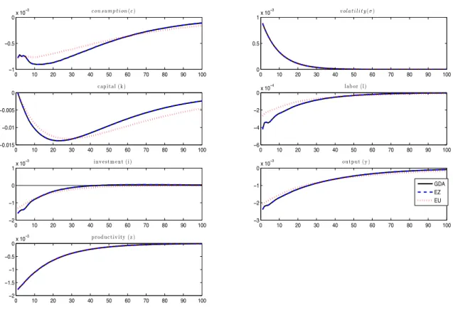
0 10 20 30 40 50 60 70 80 90 100

−1

−0.5 0x 10

−3 _{c o n s u m p t i o n}₍_c₎

0 10 20 30 40 50 60 70 80 90 100

0 0.5

1x 10

−3 _{v o l a t i l i t y}₍σ)

0 10 20 30 40 50 60 70 80 90 100

−0.015

−0.01

−0.005 0

c ap ital (k )

0 10 20 30 40 50 60 70 80 90 100

−6

−4

−2 0x 10

−4 _{lab or (l)}

0 10 20 30 40 50 60 70 80 90 100

−2

−1 0 1x 10

−3 _{i nv e stm e nt (i)}

0 10 20 30 40 50 60 70 80 90 100

−3

−2

−1 0x 10

−3 _{ou tp u t (y )}

0 10 20 30 40 50 60 70 80 90 100

−2

−1.5

−1

−0.5 0

x 10−3 p ro d u c tiv ity (z )

GDA EZ EU

Figure 6: Impulse Response Functions to both shocks minus IRFs to productivity shock alone: In the solid black line, we have the IRF for the model with GDA (a = 0.3), in the dashed line, the IRF for

the Epstein-Zin-Weil model (a= 1) and, in the dotted line, the IRF for the model with expected utility

(a= 1 andψ= 0.4).

Once again, we have that the effect of the shock on all variables is the same in the models with Epstein-Zin-Weil preferences and with GDA. Also, since the agent with expected utility prefers to smooth consumption over time, the shock has less impact on economic activity in this model.

6 Asset Pricing Implications

In this section, we present the asset pricing implications of our baseline model, as well as those of the models with Epstein-Zin-Weil preferences and expected utility. For simplicity, we price a consumption claim. For this purpose, we simulate the economy for 2000 periods and use the stochastic discount factor implied by these models to price a claim to consumption. The results of this exercise are summarized in table 2.

(22)

Table 2: Asset Pricing Implications

GDA EZW EU

E_[R_m₋_R_f_] _2.93 _0.16 _0.23

σ[Rm] 1.5 1.5 1.7

E_[R_f_]₋₁ _0.9 _1.15 _1.14

σ[Rf] 0.3 0.2 0.7

models.

However, we obtain extremely low values for the volatility of returns, not only in the GDA model, but also with Epstein-Zin-Weil and expected utility. As we know, it is difficult to match the volatility of returns (see, for instance, Campbell [2002]). Also, since consumption is smoother that stock returns, the fact that we are pricing a consumption claim contributes to lowering these second moments.

For the models with Epstein-Zin-Weil preferences and expected utility, we obtain 0.16% and 0.23% respectively. As in Bonomo et al. [2011], we find that GDA preferences yield superior asset pricing results, even in an economy with production.

Generally speaking, including production adds to the chalenge of matching asset pricing stylized facts, since these macroeconomic models imply that asset prices are extremely stable (Campbell [2002]). The real interest rate equals the marginal product of capital and, hence, is disturbed only by productivity shocks and changes in capital. Also, since we calibrate the model to match observations of the US economy, the interest rate is only a few basis points. The return on capital is also stable since capital can be costlessly transformed into goods.

7 Conclusion

In this work, we investigated the effects of volatility shocks on economic activity in the context of a real business cycle model with preferences that display generalized disap-pointment aversion and stochastic volatility in the process for productivity. We find that a shock to the volatility of productivity, when combined with a negative productivity shock, has a negative impact on economic activity. We also find that a volatility shock alone has no impact in this model.

(23)

utility. In future work, we plan to investigate the convergence issues we face in the GDA model and hopefully determine whether these preferences can be an aid to obtaining real effects to volatility shocks.

(24)

References

Ravi Bansal and Amir Yaron. Risks for the long run: A potential resolution of asset pricing puzzles. Journal of Finance, 59(4), August 2004.

Ravi Bansal, Dana Kiku, Ivan Shaliastovich, and Amir Yaron. Volatility, the macroecon-omy and asset prices. Working Paper 18104, National Bureau of Economic Research, May 2012. URL http://www.nber.org/papers/w18104.

Nicholas Bloom. The impact of uncertainty shocks. Econometrica, 77(3):623–685, 05 2009.

Marco Bonomo, Rene Garcia, Nour Meddahi, and Romeo Tedongap. Generalized disap-pointment aversion, long run volatility risk and asset prices. The Review of Financial

Studies, 24(1), 2011.

Dario Caldara, Jesus Fernandez-Villaverde, Juan Rubio-Ramirez, and Wen Yao. Com-puting dsge models with recursive preferences. Review of Economic Dynamics, (15), October 2012.

John Y. Campbell. Consumption-based asset pricing. Technical report, 2002.

Lawrence Christiano, Roberto Motto, and Massimo Rostagno. Financial factors in eco-nomic fluctuations. Working Paper Series 1192, European Central Bank, May 2010. Larry Epstein and Stanley Zin. Risk aversion, and the temporal behavior of consumption

and asset returns: A theoretical framework. Econometrica, 57(4), June 1989.

Jesus Fernandez-Villaverde and Juan Rubio-Ramirez. Macroeconomics and volatility: Data, models, and estimation. NBER Working Papers 16618, National Bureau of

Eco-nomic Research, Inc, December 2010. URLhttp://ideas.repec.org/p/nbr/nberwo/16618.html. Jesus Fernandez-Villaverde and Juan F. Rubio-Ramirez. Estimating macroeconomic

models: A likelihood approach. Review of Economic Studies, 74(4):1059–1087, Oc-tober 2007.

Jesus Fernandez-Villaverde, Pablo Guerron-Quintana, Juan Rubio-Ramirez, and Martin Uribe. Risk matters: The real effects of volatility shocks. American Economic Review, 101(6), October 2011.

(25)

Rubio-11-022, Penn Institute for Economic Research, Department of Economics, University of Pennsylvania, August 2012. URLhttp://ideas.repec.org/p/pen/papers/11-022.html. Faruk Gul. A theory of disappointment aversion. Econometrica, (57):357–384, 1991.

Lars Peter Hansen, John C. Heaton, and Nan Li. Consumption strikes back? mea-suring long-run risk. Journal of Political Economy, 116(2):260–302, 04 2008. URL

http://ideas.repec.org/a/ucp/jpolec/v116y2008i2p260-302.html.

Alejandro Justiniano and Giorgio E. Primiceri. The time-varying volatility of macroeco-nomic fluctuations. American Economic Review, 98(3):604–41, June 2008.

Emi Nakamura, Dmitriy Sergeyev, and Jn Steinsson. Growth-rate and uncertainty shocks in consumption: Cross-country evidence. Working Paper 18128, National Bureau of Economic Research, June 2012.

Bryan R. Routledge and Stanley E. Zin. Generalized disappointment aversion and asset prices. Journal of Finance, (65):1303–1332, 2010.

George Tauchen. Finite state markov-chain approximations to univariate and vector

au-toregressions.Economics Letters, 20(2):177–181, 1986. URLhttp://ideas.repec.org/a/eee/ecolet/v20y1986i2p177-181.html