Carlos Pestana Barros & Nicolas Peypoch
A Comparative Analysis of Productivity Change in Italian and
Portuguese Airports
WP 006/2007/DE
_________________________________________________________
António Afonso & Ana Sequeira
Revisiting business cycle synchronisation in the European
Union
WP 22/2010/DE/UECE
_________________________________________________________
Department of Economics
W
ORKING
P
APERS
ISSN
Nº0874-4548
School of Economics and Management
Revisiting business cycle synchronisation
in the European Union
*
António Afonso
$
#
,
Ana Sequeira
2010
Abstract
We assess the business cycle synchronization features of aggregate output in the 27 EU
countries using annual data for the period 1970-2009. In particular, we compute
measures of synchronisation for private consumption, government spending, gross fixed
capital formation, exports and imports. Our results show a rise in synchronization over
the full period, and although private consumption is the biggest component of GDP,
external demand tends to be a more important determinant of business cycle
synchronization.
JEL: E32; F15; F41; F42
Keywords: EU, business cycle synchronization.
*
The opinions expressed herein are those of the authors and do not necessarily reflect those of the ECB or
the Eurosystem.
$
ISEG/TULisbon – Technical University of Lisbon, Department of Economics; UECE – Research Unit
on Complexity and Economics, R. Miguel Lupi 20, 1249-078 Lisbon, Portugal, email:
aafonso@iseg.utl.pt. UECE is supported by FCT (Fundação para a Ciência e a Tecnologia, Portugal),
financed by ERDF and Portuguese funds.
#
European Central Bank, Directorate General Economics, Kaiserstraße 29, D-60311 Frankfurt am Main,
Germany, emails: antonio.afonso@ecb.europa.eu.
1. Introduction
In the context of the European and Monetary Union (EMU) and of the broader
setting of the European Union (EU) itself, the existence of a higher degree of business
cycle synchronisation seems to be an expected outcome of European integration. An
increase in the correlation of the cyclical fluctuations may reduce the potential costs of
the inexistence of country-specific monetary policies, in the case of the EMU.
Moreover, the presence of high business cycle correlation between countries and the
EMU aggregates also helps the implementation of monetary policy conducted by the
European Central Bank. Indeed, the theory of the Optimum Currency Area, first
developed by Mundell (1961), McKinnon (1963) and Kenen (1969), stresses the
importance of international linkages between the members of a monetary union to deal
with the loss of the country-specific monetary policy to address the economic business
cycle.
In this paper we analyse business cycle synchronization in the EU, notably by
assessing how it has evolved over time, using annual data for the period 1970-2009.
Specifically we look at business cycle synchronisation of both GDP and of aggregate
demand components: private consumption, final consumption expenditure of general
government, gross fixed capital formation, and exports and imports of goods and
services. We also determine which aggregated demand component sector mostly drives
GDP business cycle synchronization.
In a nutshell, the results show that the level of business cycle synchronization for the
27 EU countries has increased between 1970 and 2009. Notably, it has been higher after
the introduction of the single currency. In the most recent 1993-2008 sub-period, some
of the new Member States (Cyprus, Latvia and Slovenia) already presented business
cycle synchronization similar to that of some EU-15, namely comparing to Greece and
Portugal.
The remainder of the paper is organized as follows. Section Two provides a brief
review of related literature. Section Three explains the empirical methodology used to
compute business cycle synchronization. Section Four reports the results obtained, and
Section Five summarises the paper’s main findings.
2. Related literature
(1999) describe the rise of the output correlation between Germany and the other
European countries, particularly in the period 1993-1997. Furceri and Karras (2008)
focus on business cycle synchronization for GDP components, using data for the period
1993-2004 (EU with 12 member states), and conclude the countries observed are better
synchronized with the EMU-wide economy after joining the Euro. Moreover, the
aggregate demand components best synchronized are exports and imports.
Afonso and Furceri (2009) evaluate the sectoral business cycle synchronization in
the EU (27 member states) for the period 1980-2005 and conclude that, in general,
Industry, Building and Construction and Agriculture, Fishery and Forestry give the best
contribution to aggregate output business cycle synchronization, while Services show
low business cycle synchronization.
Several authors have also investigated the evolution of business cycle
synchronization in North-America. Lopes and Pina (2008) use fuzzy clustering and
rolling window techniques to compare Europe with two other currency unions - Canada
and the USA - for what business cycle synchronization and core-periphery patterns are
concerned. This study reveals that EMU is economically viable, once the average
cyclical correlations among European countries have developed in a positive and
significant way (assuming very near or superior values to those found for North
American regions). On the other hand, Wynne and Koo (2000) compare the business
cycle in the European Union (15 member states) with the business cycle in twelve
Federal Reserve districts in the U.S., concluding that synchronization in the USA is
higher than in Europe, for the period 1963-1992. Clark and Wincoop (2001) try to
understand the border effect analyzing the US-Canada border and inter-European
borders, concluding that it not only exists in Europe, but is also statistically significant
in this case.
Other studies document the evolution of business cycle synchronization over time.
Gayer (2007) analyzes industrial production and GDP, and verifies that business cycle
synchronization in the euro area has been rising since the euro introduction (although
inferior to the synchronization level showed in the early 1990s). Fatás (1997), using
annual data for the period 1966-1992, studies the evolution of business cycle
synchronization between EU countries or regions. Calculating the correlations of
growth rates of employment, he identifies a rise in cross-country correlations and a fall
between same-country regions. In addition, Peiró (2004) studied the existence of
Mink et al. (2007) expose a new cycle co-movement measure which allows them to
determine the synchronization of cycles and the differences between their amplitudes.
Applying it to euro area data for the period between 1970 and 2005, they argue that
business cycle synchronization and co-movement do not show an upward trend, and
countries presenting the lowest values for these variables are Finland, Greece and Italy.
Some other papers study business cycle correlation between the euro area and
acceding countries. Korhonen (2003) uses an econometric study to gauge the integration
level of nine country-candidates with the euro area, concluding that Greece and Portugal
are as integrated as some of the most advanced country-candidates, namely Hungary
and Slovenia. Artis et al. (2004) examine the evolution of the business cycle in the
accession countries and find evidence of a weak synchronization, excluding the cases of
Poland and Hungary.
Using a model-based clustering, Crowley (2008) shows that macroeconomic
variables evolved in a divergent way within the euro area and reports the existence of a
geographical core-periphery pattern. Normalizing distances between the leading country
and the rest of countries, and afterward generating values using a bivariate uniform
distribution, as well as a bivariate normal distribution, Camacho et al. (2006) conclude
that there is no evidence proving the existence of any attractor or common driving force
in economic cycles of European countries. Finally, Inklaar and Haan (2001) do not find
any evidence of a connection between exchange rate stability and business cycle
synchronization in Europe.
3. Methodology
We compute our business cycle measures for GDP as the correlation between the
country’s GDP cyclical component,
c
i, and the EU’s GDP cyclical component,c
EU:
i,
EU
corr c c
.
(1)
In addition, and to assess which aggregate demand component
j
for each country
i
is
mainly responsible for the aggregate output business cycle synchronization, we compute
the country’s aggregate demand cyclical components,
c
ij, and then calculate the
ij,
EU
corr c c
.
(2)
We used the HP filter (Hodrick and Prescott, 1980) with the smoothness parameters
equal to 100 and 6.25 to compute the cyclically adjusted components of aggregate
demand as well as the corresponding component of GDP.
As a robustness measure, and given some of the critics to different de-trending
techniques, as the HP filter (see Canova (1998), we also calculate the Business Cycle
Synchronization using a so-called Business Cycle Synchronization Index (BSCI).
According to Kalemli-Ozcan et al. (2010) e Giannone et al. (2008), this new measure
evaluates the cross-country synchronization (between countries
i
and
j
) to the same
variable. Considering
S
ijt a negative of the divergence in growth rates, defined as theabsolute value of GDP (or other aggregate demand components), growth differences
between countries
i
and
j
in year
t
are given by:
1 1
(ln
ln
) (ln
ln
)
ijt it it jt jt
S
Y
Y
Y
Y
.
(3)
where
Y
it is real GDP of countryi
in period
t
.
In our analysis we will apply this measure to study synchronization between the real
GDP of country
i
and the real GDP of the euro area. Since we will report the results per
period of time, each value will match to the average of obtained values for each one of
these periods.
4. Empirical analysis
4.1. Data
Our data come from the European Commission
Annual Macro-economic Database
(AMECO) and covers the EU 27 countries from 1970 to 2009, as far as data availability
allows for.
1We use real GDP at 2000 constant prices to compute output business cycle
synchronization, and we consider as well the following aggregate demand components:
private consumption, final consumption expenditure of general government, gross fixed
capital formation, and exports and imports of goods and services.
1
4.2. Output Business Cycle Synchronization
In order to analyze the business cycle synchronization across a set of European
countries, we first computed the correlation coefficient between the cyclical component
of real GDP in country
i
, and the cyclical component of real GDP in the euro area
(defined for this purpose as the 12 “old” initial euro area countries). We used the HP
filter with the smoothness parameter equal to 100 to disentangle between cycle and
trend. Naturally, the higher the correlation coefficient the higher the business cycle
synchronization.
In this study we use annual data and cover the period time between 1970 and 2009.
In order to segment and deepen our analysis, we have divided the overall period in three
sub-periods: the first one from 1970 to 1992 – where we hardly observe values for the
last group of countries that joined the EU; the second one from 1993 to 1998 – allowing
us to check the possible Maastricht treaty’s effects on synchronization; and the last one,
from 1999 to 2009 – where we analyze the consequences of the adoption of the single
currency. For the last two sub-periods, we are already able to present values regarding
the current 27 members of EU.
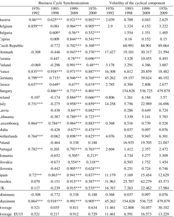
We report in Table 1 the results for business cycle synchronisation for the 27 EU
countries, vis-à-vis the euro area (EA12).
2It is possible to observe that the level of
business cycle synchronization has increased, notably between 1970-1992 and
1999-2009. Analyzing column four of Table 1, for the full period, we can conclude that most
countries are relatively well synchronized with the euro area, being that of the fifteen
initial EU countries, only four (Denmark, Finland, UK and Sweden) have correlations
below the average.
In the sub-period of 1970 to 1992, we notice that although there were already
countries with a high level of business cycle synchronization (such as Austria, Belgium,
France and Luxembourg), in some cases business cycle synchronization was extremely
low (Ireland, Sweden, U.K.) or even negative (Denmark, Finland).
Comparing the values obtained in the two sub-first periods, we notice a decrease in
synchronization from the first one to the second one. Only Spain and France present
positive variations. However, we should take into account that the period between 1993
and 1998 covers only six years.
Table 1 – GDP Business cycle synchronization (vis-à-vis EA12)
Note: Hodrick-Prescott Filter with smoothness parameter equal to 100.
***,**,* denote significance respectively at 1%, 5%, and 10%.
In the more recent period between 1999 and 2009, all countries depict a high level
synchronization with the euro area. Below average synchronization is reported for
several EU New Member States (notably Poland, with the lowest synchronization,
Bulgaria and Romania), and Greece. Interestingly, Cyprus, Latvia and Slovenia already
showed a correlation above the average. Indeed, several countries outside the euro area
Business Cycle Synchronization
Volatility of the cyclical component
1970-1992
1993-1998
1999-2009
1970-2009
1970-1992
1993-1998
1999-2009
in that sub-period had already a higher economic synchronization than some euro area
countries (Greece and Portugal, for instance), in line with Korhonen (2003).
Table 1 also shows the volatility of the correlation coefficients that measure the
respective business cycle synchronisation. We can then see that the average volatility
increased throughout the three sub-periods. In the first sub-period, business cycle
volatility ranged between Luxembourg and Ireland and Germany, which had the lowest
volatility level. Between 1993 and 1998, countries like Austria, Cyprus, Greece, Latvia,
Luxembourg, Malta, Slovenia and Slovakia also presented low volatility levels, while
the opposite occurred in the case of Hungary. In the 1999-2009 sub-period the number
of countries with low business cycle volatility diminished.
In Table 2 we report the results for the Business Cycle Synchronization Index for
each of the EU Member States, taking into consideration three time periods: 1971-1992,
1993-2009 and 1971-2009 (the reason why 1971 is the first year is because all the
values obtained come from a first-order differences process).
For the first sub-period, and given that the closer BSCI is to zero, the higher will be
the synchronization between country
i
and the euro area, we observe that the countries
that were more synchronized with the euro area are France and Germany, and the least
synchronized ones were Portugal and Greece.
Between 1993 and 2009, the most synchronized countries were France (0.004),
Germany (-0.005), Belgium (-0.005), and Austria (-0.006), and the least synchronized
were Lithuania (-0.680) and Latvia (-0.062). These results are in line with conclusions
that can be drawn for the full period, and also with the overall results from Table 1,
where the HP filter was used.
Moreover, and as we have observed also in Table 1, and evaluating the evolution of
values showed in the last line of Table 2 (average to the EU-15), we can see that overall
countries have become more synchronized with the euro area over time. The same is
true for the EU New Member States, a result in line with what had been argued notably
by Rose and Engel (2002), once increased intra EU trade also increase the
Table 2 – GDP Business cycle synchronization Index (vis-à-vis EA12)
Business Cycle Synchronization Index
1971-1992
1993-2009
1971-2009
Austria
-0.013
-0.006
-0.010
Belgium
-0.008
-0.005
-0.006
Bulgaria
-0.040
-0.042
Cyprus
-0.013
-0.015
Czech Republic
-0.023
-0.027
Denmark
-0.018
-0.008
-0.013
Estonia
-0.058
-0.058
Finland
-0.019
-0.016
-0.018
France
-0.006
-0.004
-0.005
Germany
-0.007
-0.005
-0.006
Greece
-0.028
-0.016
-0.022
Hungary
-0.020
-0.020
Ireland
-0.021
-0.039
-0.029
Italy
-0.010
-0.007
-0.009
Latvia
-0.062
-0.082
Lithuania
-0.068
-0.077
Luxembourg
-0.024
-0.020
-0.022
Malta
-0.019
-0.020
Netherlands
-0.009
-0.008
-0.009
Poland
-0.033
-0.034
Portugal
-0.031
-0.008
-0.021
Romania
-0.047
-0.053
Slovakia
-0.040
-0.040
Slovenia
-0.027
-0.032
Spain
-0.014
-0.007
-0.011
Sweden
-0.015
-0.011
-0.013
UK
-0.015
-0.009
-0.012
Minimum
-0.031
-0.068
-0.082
Maximum
-0.006
-0.004
-0.005
Average
-0.016
-0.023
-0.026
Average EU15
-0.016
-0.011
-0.014
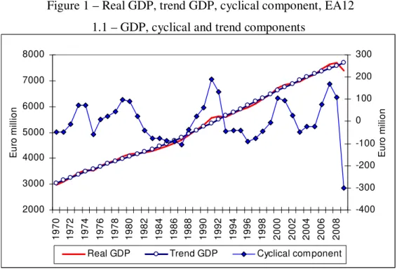
Given that we are using the 12 “old” countries of the EU to build the aggregate
cyclical components of GDP, it is worthwhile comparing the peaks and troughs that we
uncover with the ones reported by the CEPR Euro Area Cycle Dating Committee. Such
comparison is reported in Figure 1.
Interestingly, it is possible to observe that the downturns identified by the
Committee are very close to the peaks and troughs that we computed for the cyclical
Figure 1 – Real GDP, trend GDP, cyclical component, EA12
1.1 – GDP, cyclical and trend components
2000
3000
4000
5000
6000
7000
8000
1
9
7
0
1
9
7
2
1
9
7
4
1
9
7
6
1
9
7
8
1
9
8
0
1
9
8
2
1
9
8
4
1
9
8
6
1
9
8
8
1
9
9
0
1
9
9
2
1
9
9
4
1
9
9
6
1
9
9
8
2
0
0
0
2
0
0
2
2
0
0
4
2
0
0
6
2
0
0
8
E
u
ro
m
il
li
o
n
-400
-300
-200
-100
0
100
200
300
E
u
ro
m
il
io
n
Real GDP
Trend GDP
Cyclical com ponent
1.2 – Real and trend GDP growth rates, and CEPR peaks and troughs
08Q1-?
92Q1-93Q3
80Q1-82Q3
77Q3-75Q1
-4 -3 -2 -1 0 1 2 3 4 5 6 7 1 9 7 0 1 9 7 2 1 9 7 4 1 9 7 6 1 9 7 8 1 9 8 0 1 9 8 2 1 9 8 4 1 9 8 6 1 9 8 8 1 9 9 0 1 9 9 2 1 9 9 4 1 9 9 6 1 9 9 8 2 0 0 0 2 0 0 2 2 0 0 4 2 0 0 6 2 0 0 8 G ro w th r a te ( % )Real GDP
Trend GDP
Source: own computations and CEPR Euro Area Cycle Dating Committee for the euro area peaks and
troughs in chart 1.2 (http://www.cepr.org/data/dating/).
4.3. Business Cycle Synchronization by GDP components
Private Consumption synchronization
In Table 3 there are three different types of information available. The first four
columns show the correlation between the cyclical component of private consumption
in country
i
and the cyclical component of real GDP in the euro area. The next four
Table 3 present the volatilities of those private consumption business cycle correlations.
The sub-periods considered remain the same.
Table 3 – Private consumption synchronization (vis-à-vis EA12)
Business Cycle Synchronization Share in GDP (%) Volatility
of the cyclical
component
1970-1992
1993-1998
1999-2009
1970-2009
1970-1992
1993-1998
1999-2009
1970-2009
1970-1992
1993-1998
1999-2009
1970-2009
Austria 0.644*** 0.083 0.674** 0.543*** 57.8 57.7 54.2 56.8 1.324 0.884 0.733 1.108
Belgium 0.899*** 0.319 0.897*** 0.847*** 54.5 55.0 52.3 54 1.520 0.432 1.135 1.320
Bulgaria 0.411 0.624** 0.539*** 67.6 71.0 69.6 1.392 0.994 1.097
Cyprus -0.308 0.479* 0.255* 62.7 66.4 65.3 0.277 0.193 0.215
Czech Republic -0.841 0.185 -0.15 50.6 52.0 50.7 43.342 20.627 49.681
Denmark -0.188 -0.319 0.697*** 0.18 54.1 51.0 49.4 52.4 13.841 12.505 19.025 15.022
Estonia -0.165 0.77*** 0.669*** 54.5 57.9 56.7 1.532 7.539 6.055
Finland 0.066 -0.466 0.825*** 0.355** 53.2 52.5 50.7 52.4 1.733 1.673 1.326 1.786
France 0.697*** 0.601 0.829*** 0.688*** 57.6 56.3 57.4 57.3 8.134 6.115 6.093 8.759
Germany 0.68*** 0.481 0.268 0.422*** 56.2 59.4 57.9 57.2 32.150 19.328 11.352 26.183
Greece 0.641*** 0.691* 0.681** 0.657*** 64.5 75.0 72.7 68.3 2.033 0.228 2.508 2.010
Hungary 0.402 0.41 0.39*** 53.6 56.5 55.7 384.672 473.049 438.732
Ireland 0.449** 0.273 0.975*** 0.786*** 63.2 52.1 47.5 57.2 0.792 0.440 2.715 1.623
Italy 0.741*** 0.365 0.833*** 0.737*** 58.4 58.9 59.6 58.8 10.164 7.053 8.706 10.431
Latvia -0.51 0.818*** 0.702*** 64.1 65.7 65.3 0.119 0.573 0.492
Lithuania -0.087 0.785*** 0.669*** 61.2 66.6 65.1 0.767 4.172 3.594
Luxembourg 0.788*** 0.625* 0.29 0.543*** 53.4 44.5 38.6 48.0 0.125 0.081 0.232 0.162
Malta -0.921 0.327 0.362** 65.0 66.5 66.1 0.031 0.053 0.050
Netherlands 0.61*** -0.049 0.566** 0.605*** 54.2 50.0 49.1 52.2 3.292 2.215 4.495 3.826
Poland -0.419 0.075 0.163 64.1 63.9 63.6 8.746 9.439 8.669
Portugal 0.798*** 0.568 0.688*** 0.705*** 58.5 63.6 65.2 61.1 1.751 1.157 1.130 1.539
Romania -0.747 0.6** 0.392*** 63.2 79.7 71.8 3.263 7.155 6.030
Slovakia -0.509 0.445* 0.226* 45.3 55.5 52.4 0.328 0.522 0.490
Slovenia -0.477 0.683** 0.094 59.0 55.7 56.2 0.170 0.207 0.338
Spain 0.797*** 0.713* 0.891*** 0.852*** 62.0 59.9 59.7 61.1 8.319 4.089 12.449 9.631
Sweden 0.353** 0.085 0.883*** 0.542*** 54.1 50.2 48.6 52.0 25.197 5.969 17.764 24.391
UK 0.212 0.271 0.749*** 0.501*** 59.6 63.5 66.4 62.0 12.603 3.030 14.261 13.235
Minimum -0.188 -0.921 0.075 -0.15 53.2 44.5 38.6 48 0.125 0.031 0.053 0.050
Maximum 0.899*** 0.713*** 0.975*** 0.852*** 64.5 75.0 79.7 71.8 32.150 384.672 473.049 438.732
Average 0.546 0.003 0.628 0.492 57.4 57.8 58.8 58.9 8.199 18.883 23.276 23.573
Average EU15 0.546 0.283 0.716 0.598 57.4 56.6 55.3 56.7 8.199 4.347 6.928 8.068
Note: Hodrick-Prescott Filter with smoothness parameter equal to 100.
***,**,* denote significance respectively at 1%, 5%, and 10%.
For the period from 1970 to 1992, only Denmark presented a small negative private
consumption synchronization (although not statistically significant) with the euro area.
sub-period, most countries presented high synchronization values, although to less extent in
the cases Poland, Czech Republic, Germany, Malta and Luxembourg.
Considering the contribution of private consumption to GDP, we can see that it has
barely changed throughout time, representing on average a somewhat between 57% and
59% of GDP. At the country level, and apart from the EU New Member States, only
Italy, Portugal and the UK had an increase if the contribution to GDP of private
consumption. Is some cases such share decreased, notably in France, with a negative
variation from the first to the second sub-period, and a positive one from the second to
the third, while the opposite occurred in Belgium, Germany and Greece. In all the other
countries the share of private consumption in GDP decreased.
Regarding the volatilities of private consumption business cycle correlations, in the
first sub-period, those countries that were best synchronized with the euro area
presented themselves with lower volatility values as well. Between 1993 and 1998, the
volatilities of the correlations between the consumption of country
i
and the GDP in
euro area decreased, except in the cases of the Czech Republic and Hungary. In the last
sub-period period, volatilities have increased for most countries, as we have observed
for the case of GDP as well.
Final Consumption Expenditure of General Governments synchronization
Table 4 shows the same kind of information for the final consumption expenditure
of general government, as it was previously presented for private consumption.
In this case, government spending represents, on average, around 20% of the GDP.
In every period under analysis, Sweden is the country with the highest share of
government spending in GDP. Interestingly, the New EU Member States show similar
characteristics and behaviour as in the case of the other EU countries.
For the overall period we can see that public expenditure synchronization with GDP
in the euro area was positive (and statistically significant) for Bulgaria, Greece, Ireland,
Italy, the Netherlands, Poland Portugal, Spain, and Sweden. To some extent, we see in
these cases the existence of some pro-cyclicality of government spending, which one
would not expect to help fiscal sustainability. Negative correlations are uncovered for
Table 4 – Final consumption expenditure of general government synchronization
(vis-à-vis EA12)
Business Cycle Synchronization Share in GDP (%) Volatility
of the cyclical
component
1970-1992
1993- 1998
1999-2009
1970-2009
1970-1992
1993- 1998
1999-2009
1970-2009
1970-1992
1993-1998
1999-2009
1970-2009
Austria -0.047 0.203* -0.133 -0.147 18.1 20.0 18.9 18.6 0.437 0.711 0.752 0.592
Belgium 0.108 -0.674 -0.617 -0.093 21.3 21.4 22.5 21.7 0.844 0.460 0.621 0.737
Bulgaria 0.91* 0.076* 0.412*** 15.2 17.4 16.9 0.709 0.242 0.528
Cyprus -0.626 -0.55 -0.511 15.6 18.1 17.4 0.053 0.078 0.070
Czech Republic -0.098* 0.042 0.047 21.3 21.5 21.6 12.656 14.405 24.148
Denmark -0.271 0.122 -0.598 -0.308 24.8 25.5 26.4 25.4 5.084 2.443 3.668 4.368
Estonia 0.273 0.307 0.187 22.6 18.7 20.1 0.807 1.045 0.964
Finland 0.503*** -0.829 -0.518 0.158 19.1 22.9 21.8 20.4 0.663 0.344 0.544 0.617
France -0.151 0.142*** 0.044 -0.073 20.9 23.7 23.4 22.0 3.122 4.438 3.456 3.359
Germany 0.507*** 0.172*** -0.548* 0.14 18.8 19.5 18.8 18.9 11.906 5.914 5.593 9.857
Greece -0.256 0.3 0.341* 0.21* 13.6 14.8 17.1 14.7 0.523 0.524 0.999 0.772
Hungary 0.601*** 0.212 -0.19 24.5 22.0 23.1 433.067 182.015 546.750
Ireland 0.172 0.382*** 0.64 0.443*** 17.2 15.9 15.4 16.5 0.369 0.379 0.662 0.461
Italy 0.591*** 0.287** 0.136* 0.435*** 17.8 18.6 19.7 18.5 5.469 5.759 4.476 5.581
Latvia 0.438 0.523 0.204 21.0 19.8 18.6 0.065 0.078 0.076
Lithuania -0.3 0.362 -0.024 23.1 20.5 20.6 1.277 0.483 1.419
Luxembourg 0.577*** 0.035*
-0.531** 0 15.1 16.0 16.0 15.5 0.063 0.058 0.123 0.083
Malta -0.932
-0.474** -0.561 19.0 20.2 19.4 0.016 0.032 0.027
Netherlands 0.528*** 0.72** 0.155 0.337** 23.1 23.2 24.2 23.4 1.354 1.823 2.023 1.588
Poland -0.248 0.156 0.45*** 18.7 18.0 18.8 3.901 3.611 4.675
Portugal 0.751*** 0.416** -0.205 0.36** 13.8 18.0 20.4 16.3 0.561 0.501 0.614 0.570
Romania 0.223** 0.265 0.253* 13.4 16.7 15.8 1.261 1.104 1.106
Slovakia -0.614 -0.04 -0.189 22.9 19.3 20.6 0.405 0.238 0.314
Slovenia 0.482***
-0.237** 0.062 18.7 18.8 18.6 0.062 0.073 0.074
Spain 0.709*** 0.473*** -0.284 0.238* 13.8 18.0 18.1 15.6 2.089 2.831 2.230 2.197
Sweden 0.596*** 0.301 0.249 0.488*** 26.4 27.4 26.7 26.6 10.840 7.446 7.446 10.082
UK 0.236 0.352*** -0.204* 0.102 20.6 19.1 20.6 20.4 3.283 5.818 4.806 4.242
Minimum -0.271 -0.932 -0.617 -0.561 13.6 13.4 15.4 14.7 0.063 0.016 0.032 0.027
Maximum 0.751*** 0.91*** 0.64*** 0.488*** 26.4 27.4 26.7 26.6 11.906 433.067 182.015 546.750
Average 0.304 0.093 -0.053 0.09 19.0 20.0 20.0 19.5 3.107 18.286 8.941 23.158
Average EU15 0.304 0.160 -0.138 0.153 19.0 20.3 20.7 19.6 3.107 2.630 2.534 3.007
Note: Hodrick-Prescott Filter with smoothness parameter equal to 100.
***,**,* denote significance respectively at 1%, 5%, and 10%.
Regarding the evolution on private consumption synchronization over time, it
varied negatively in the elder members of the EU (except for France, Greece and
Ireland), and positively for the New Member States (excluding Bulgaria, Hungary and
When we look to the volatility levels, the Czech Republic and Hungary have the
highest values, and, interestingly, high levels of volatility also occurred in the period
1993-1998.
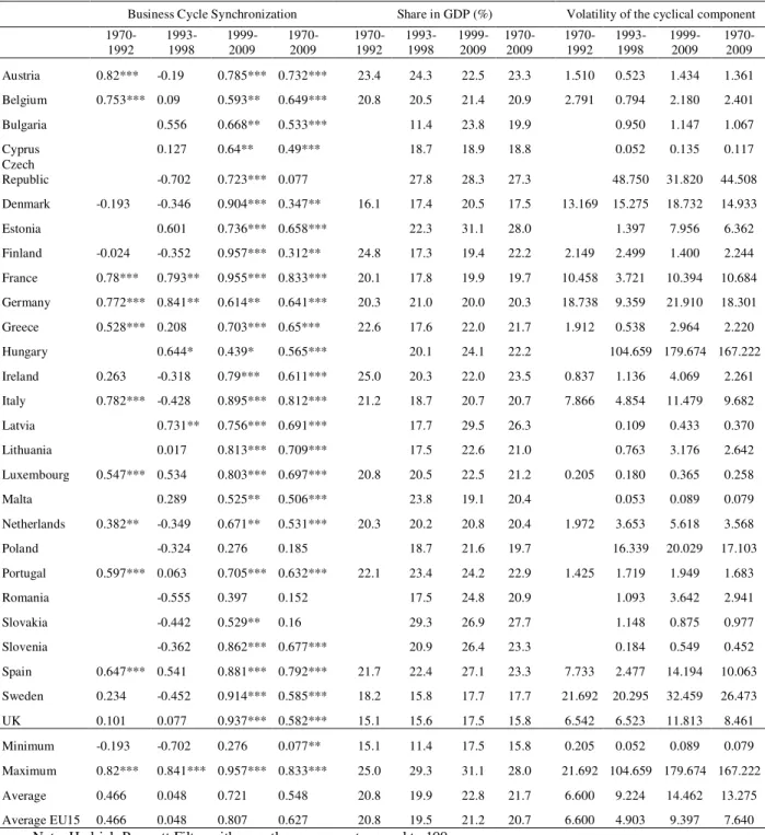
Gross Fixed Capital Formation synchronization
Table 5 shows the investment component of GDP, more precisely gross fixed
capital formation (GFCF).
During the period 1970-2009, GFCF synchronization with euro area GDP was
rather high for many countries (notably France, Italy, and Spain), although there are also
low synchronization levels, such as the case of Denmark and Finland. In the period
1993-1998, only France and Germany presented a positive variation from the first
sub-period to the second one. Between 1999 and 2009, the lower levels of GFCF business
cycle synchronisation were the New Member States like the Czech Republic, Bulgaria
and Slovakia. Finland and Denmark also present low correlations. On the other hand,
the best synchronized countries were France and Italy.
GFCF is responsible, on average, for around 21% of GDP. For the sub-period
1999- 2009, the U.K. is the country in which the investment’s share in GDP is the
lowest (17.5%), while Estonia had the highest level (31.1%).
Again, from the last four columns in 5, we observe an increase in business cycle
volatility, with the Czech Republic, Hungary and Sweden, with the highest volatility
Table 5 – Gross fixed capital formation synchronization (vis-à-vis EA12)
Business Cycle Synchronization Share in GDP (%) Volatility of the cyclical component
1970-1992
1993-1998
1999-2009
1970-2009
1970-1992
1993-1998
1999-2009
1970-2009
1970-1992
1993-1998
1999-2009
1970-2009
Austria 0.82*** -0.19 0.785*** 0.732*** 23.4 24.3 22.5 23.3 1.510 0.523 1.434 1.361
Belgium 0.753*** 0.09 0.593** 0.649*** 20.8 20.5 21.4 20.9 2.791 0.794 2.180 2.401
Bulgaria 0.556 0.668** 0.533*** 11.4 23.8 19.9 0.950 1.147 1.067
Cyprus 0.127 0.64** 0.49*** 18.7 18.9 18.8 0.052 0.135 0.117
Czech
Republic -0.702 0.723*** 0.077 27.8 28.3 27.3 48.750 31.820 44.508
Denmark -0.193 -0.346 0.904*** 0.347** 16.1 17.4 20.5 17.5 13.169 15.275 18.732 14.933
Estonia 0.601 0.736*** 0.658*** 22.3 31.1 28.0 1.397 7.956 6.362
Finland -0.024 -0.352 0.957*** 0.312** 24.8 17.3 19.4 22.2 2.149 2.499 1.400 2.244
France 0.78*** 0.793** 0.955*** 0.833*** 20.1 17.8 19.9 19.7 10.458 3.721 10.394 10.684
Germany 0.772*** 0.841** 0.614** 0.641*** 20.3 21.0 20.0 20.3 18.738 9.359 21.910 18.301
Greece 0.528*** 0.208 0.703*** 0.65*** 22.6 17.6 22.0 21.7 1.912 0.538 2.964 2.220
Hungary 0.644* 0.439* 0.565*** 20.1 24.1 22.2 104.659 179.674 167.222
Ireland 0.263 -0.318 0.79*** 0.611*** 25.0 20.3 22.0 23.5 0.837 1.136 4.069 2.261
Italy 0.782*** -0.428 0.895*** 0.812*** 21.2 18.7 20.7 20.7 7.866 4.854 11.479 9.682
Latvia 0.731** 0.756*** 0.691*** 17.7 29.5 26.3 0.109 0.433 0.370
Lithuania 0.017 0.813*** 0.709*** 17.5 22.6 21.0 0.763 3.176 2.642
Luxembourg 0.547*** 0.534 0.803*** 0.697*** 20.8 20.5 22.5 21.2 0.205 0.180 0.365 0.258
Malta 0.289 0.525** 0.506*** 23.8 19.1 20.4 0.053 0.089 0.079
Netherlands 0.382** -0.349 0.671** 0.531*** 20.3 20.2 20.8 20.4 1.972 3.653 5.618 3.568
Poland -0.324 0.276 0.185 18.7 21.6 19.7 16.339 20.029 17.103
Portugal 0.597*** 0.063 0.705*** 0.632*** 22.1 23.4 24.2 22.9 1.425 1.719 1.949 1.683
Romania -0.555 0.397 0.152 17.5 24.8 20.9 1.093 3.642 2.941
Slovakia -0.442 0.529** 0.16 29.3 26.9 27.7 1.148 0.875 0.977
Slovenia -0.362 0.862*** 0.677*** 20.9 26.4 23.3 0.184 0.549 0.452
Spain 0.647*** 0.541 0.881*** 0.792*** 21.7 22.4 27.1 23.3 7.733 2.477 14.194 10.063
Sweden 0.234 -0.452 0.914*** 0.585*** 18.2 15.8 17.7 17.7 21.692 20.295 32.459 26.473
UK 0.101 0.077 0.937*** 0.582*** 15.1 15.6 17.5 15.8 6.542 6.523 11.813 8.461
Minimum -0.193 -0.702 0.276 0.077** 15.1 11.4 17.5 15.8 0.205 0.052 0.089 0.079
Maximum 0.82*** 0.841*** 0.957*** 0.833*** 25.0 29.3 31.1 28.0 21.692 104.659 179.674 167.222
Average 0.466 0.048 0.721 0.548 20.8 19.9 22.8 21.7 6.600 9.224 14.462 13.275
Average EU15 0.466 0.048 0.807 0.627 20.8 19.5 21.2 20.7 6.600 4.903 9.397 7.640
Note: Hodrick-Prescott Filter with smoothness parameter equal to 100.
***,**,* denote significance respectively at 1%, 5%, and 10%.
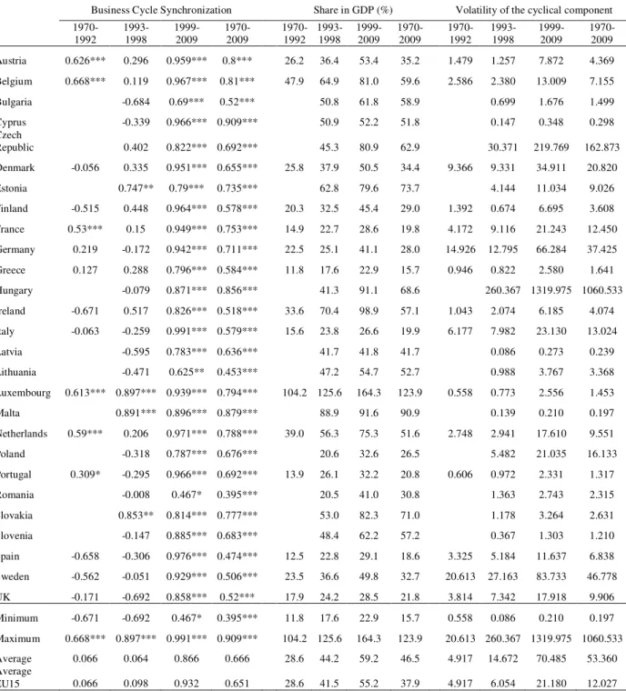
Exports and Imports of goods and services synchronization
In Table 6 we report the results related to business cycle synchronization,
volatility and the share of exports in GDP. A relevant issue is the rapid growth of
average share of exports in GDP between 1970 and 2009. This evolution may be
explained by a higher level of market integration and the introduction of the single
Table 6 – Exports of goods and services synchronization (vis-à-vis AE12)
Business Cycle Synchronization Share in GDP (%) Volatility of the cyclical component
1970-1992
1993-1998
1999-2009
1970-2009
1970-1992
1993-1998
1999-2009
1970-2009
1970-1992
1993-1998
1999-2009
1970-2009
Austria 0.626*** 0.296 0.959*** 0.8*** 26.2 36.4 53.4 35.2 1.479 1.257 7.872 4.369
Belgium 0.668*** 0.119 0.967*** 0.81*** 47.9 64.9 81.0 59.6 2.586 2.380 13.009 7.155
Bulgaria -0.684 0.69*** 0.52*** 50.8 61.8 58.9 0.699 1.676 1.499
Cyprus -0.339 0.966*** 0.909*** 50.9 52.2 51.8 0.147 0.348 0.298
Czech
Republic 0.402 0.822*** 0.692*** 45.3 80.9 62.9 30.371 219.769 162.873
Denmark -0.056 0.335 0.951*** 0.655*** 25.8 37.9 50.5 34.4 9.366 9.331 34.911 20.820
Estonia 0.747** 0.79*** 0.735*** 62.8 79.6 73.7 4.144 11.034 9.026
Finland -0.515 0.448 0.964*** 0.578*** 20.3 32.5 45.4 29.0 1.392 0.674 6.695 3.608
France 0.53*** 0.15 0.949*** 0.753*** 14.9 22.7 28.6 19.8 4.172 9.116 21.243 12.450
Germany 0.219 -0.172 0.942*** 0.711*** 22.5 25.1 41.1 28.0 14.926 12.795 66.284 37.425
Greece 0.127 0.288 0.796*** 0.584*** 11.8 17.6 22.9 15.7 0.946 0.822 2.580 1.641
Hungary -0.079 0.871*** 0.856*** 41.3 91.1 68.6 260.367 1319.975 1060.533
Ireland -0.671 0.517 0.826*** 0.518*** 33.6 70.4 98.9 57.1 1.043 2.074 6.185 4.074
Italy -0.063 -0.259 0.991*** 0.579*** 15.6 23.8 26.6 19.9 6.177 7.982 23.130 13.024
Latvia -0.595 0.783*** 0.636*** 41.7 41.8 41.7 0.086 0.273 0.239
Lithuania -0.471 0.625** 0.453*** 47.2 54.7 52.7 0.988 3.767 3.368
Luxembourg 0.613*** 0.897*** 0.939*** 0.794*** 104.2 125.6 164.3 123.9 0.558 0.773 2.556 1.453
Malta 0.891*** 0.896*** 0.879*** 88.9 91.6 90.9 0.139 0.210 0.197
Netherlands 0.59*** 0.206 0.971*** 0.788*** 39.0 56.3 75.3 51.6 2.748 2.941 17.610 9.551
Poland -0.318 0.787*** 0.676*** 20.6 32.6 26.5 5.482 21.035 16.133
Portugal 0.309* -0.295 0.966*** 0.692*** 13.9 26.1 32.2 20.8 0.606 0.972 2.331 1.317
Romania -0.008 0.467* 0.395*** 20.5 41.0 30.8 1.363 2.743 2.315
Slovakia 0.853** 0.814*** 0.777*** 53.0 82.3 71.0 1.178 3.264 2.631
Slovenia -0.147 0.885*** 0.683*** 48.4 62.2 57.2 0.367 1.303 1.210
Spain -0.658 -0.306 0.976*** 0.474*** 12.5 22.8 29.1 18.6 3.325 5.184 11.637 6.838
Sweden -0.562 -0.051 0.929*** 0.506*** 23.5 36.6 49.8 32.7 20.613 27.163 83.733 46.778
UK -0.171 -0.692 0.858*** 0.52*** 17.9 24.2 28.5 21.8 3.814 7.342 17.918 9.906
Minimum -0.671 -0.692 0.467* 0.395*** 11.8 17.6 22.9 15.7 0.558 0.086 0.210 0.197
Maximum 0.668*** 0.897*** 0.991*** 0.909*** 104.2 125.6 164.3 123.9 20.613 260.367 1319.975 1060.533
Average 0.066 0.064 0.866 0.666 28.6 44.2 59.2 46.5 4.917 14.672 70.485 53.360
Average
EU15 0.066 0.098 0.932 0.651 28.6 41.5 55.2 37.9 4.917 6.054 21.180 12.027
Note: Hodrick-Prescott Filter with smoothness parameter equal to 100.
***,**,* denote significance respectively at 1%, 5%, and 10%.
For the overall period, we can see that most of the countries exhibit a quite high
level of exports synchronization with GDP in the euro area, and synchronization
increased considerably since 1970. In the first sub-period, from fifteen countries
considered, seven presented negative correlations, especially Ireland and Spain.
synchronization, namely Belgium and Austria. The values related to the last period are
considerably higher. For instance, that is the case for Italy, which has a correlation
coefficient equal to 0.991 (and statistically significant).
For what concerns the respective business cycle volatilities, the average volatility
level has increased between periods, and Hungary and the Czech Republic remained the
countries with the highest synchronisation levels.
The average share of exports in GDP grew significantly between 1970 and 2009,
from 28.6% in the first period (1970-1992) to 59.2% in the last period (1999-2009).
This evolution may be explained by a higher level of market integration and the
introduction of the single currency, which naturally facilitated intra EU trade.
Moreover, it is also possible to observe that in the New Member States of the EU
the GDP export share has become rather important, surpassing in some cases the
contribution of external demand to GDP in the “old” EU members. An example is
Hungary where the contribution of exports to GDP more than doubled between
1993-1998 and 1999-2009. For Luxembourg it is interestingly to notice that the share of
exports in GDP is above 100%, which has to be seen in the light of the significant
financial services industry existent in that country,
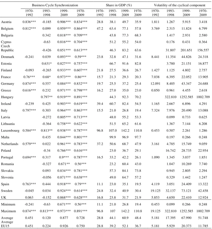
In Table 7 report the results related to business cycle synchronization, volatility and
the share of imports in GDP.
Observing the fourth column in Table 7, we can see that Belgium, France and Italy
are the countries where imports are best synchronized with GDP in the euro area.
Actually, in the first sub-period we find some countries with negative correlations (like
Denmark and Ireland), and between 1999 and 2009 the least synchronized country is
Romania, with a correlation coefficient of 0.671.
In the sub-period of 1999 to 2009, and although the New Members States are less
synchronized, the respective values are already comparable to the values of the first
fifteen members of the EU, which is a sign of increased integration with the EU.
The average imports volatilities of business cycle correlations have increased,
throughout time. Once again, Hungary and Czech Republic are cases to highlight
regarding relevant increases in GDP imports share. In addition, as in the case of the
export shares, the imports shares also increased overall. Just as we saw in the analysis
Table 7 – Imports of goods and services synchronization (vis-à-vis AE12)
Business Cycle Synchronization Share in GDP (%) Volatility of the cyclical component
1970-1992
1993-1998
1999-2009
1970-2009
1970-1992
1993-1998
1999-2009
1970-2009
1970-1992
1993-1998
1999-2009
1970-2009
Austria 0.836*** -0.185 0.906*** 0.834*** 28.8 38.1 49.7 35.9 1.811 1.267 5.915 3.418
Belgium 0.812*** 0.099 0.959*** 0.864*** 47.2 63.4 77.1 57.8 3.769 2.315 11.824 6.799
Bulgaria 0.342 0.818*** 0.709*** 43.8 77.3 68.3 1.417 2.931 2.580
Cyprus -0.63 0.816*** 0.704*** 51.2 55.2 54.0 0.176 0.431 0.364
Czech
Republic -0.426 0.851*** 0.613*** 46.3 83.2 63.6 31.807 201.651 156.557
Denmark -0.241 0.039 0.893*** 0.59*** 23.8 32.8 47.1 31.6 8.441 11.354 44.826 24.318
Estonia 0.631* 0.827*** 0.757*** 66.7 91.6 82.8 3.780 21.151 16.877
Finland -0.093 -0.265 0.933*** 0.607*** 21.8 27.5 36.6 26.7 1.427 1.125 4.802 2.757
France 0.76*** 0.68* 0.973*** 0.86*** 15.7 21.3 29.3 20.3 7.038 6.395 22.052 13.905
Germany 0.874*** 0.557 0.884*** 0.832*** 19.7 25.5 37.2 25.4 12.091 8.405 43.347 24.688
Greece 0.616*** 0.232 0.971*** 0.798*** 16.2 27.0 35.0 23.0 0.850 0.961 4.455 2.618
Hungary 0.797** 0.919*** 0.891*** 44.3 92.3 70.2 322.810 1252.585 1002.709
Ireland -0.239 0.425 0.903*** 0.619*** 39.4 60.7 82.4 54.5 1.165 2.667 6.896 4.291
Italy 0.797*** 0.303 0.964*** 0.863*** 15.5 21.0 26.8 19.4 7.324 7.976 20.490 13.088
Latvia -0.272 0.805*** 0.713*** 48.0 55.2 53.3 0.099 0.733 0.625
Lithuania -0.364 0.758*** 0.622*** 51.5 65.2 61.6 1.367 7.144 6.208
Luxembourg 0.584*** 0.813** 0.938*** 0.787*** 96.8 107.0 142.2 110.8 0.453 0.507 2.261 1.286
Malta 0.435 0.844*** 0.801*** 99.9 96.9 97.7 0.197 0.266 0.248
Netherlands 0.579*** 0.022 0.961*** 0.783*** 37.2 50.6 68.7 47.9 3.161 4.785 15.749 9.059
Poland -0.34 0.766*** 0.616*** 23.0 36.7 29.1 16.742 28.735 22.954
Portugal 0.694*** 0.317 0.9*** 0.787*** 16.5 33.2 42.2 26.1 1.090 1.345 3.037 1.851
Romania -0.327 0.671** 0.56*** 23.2 60.4 43.0 1.047 10.269 7.740
Slovakia 0.093 0.834*** 0.781*** 57.3 84.1 73.8 0.945 2.805 2.294
Slovenia -0.056 0.871*** 0.638*** 49.0 64.7 57.2 0.329 1.442 1.247
Spain 0.763*** 0.444 0.918*** 0.79*** 11.1 23.0 35.1 19.5 4.119 3.051 24.409 13.322
Sweden -0.045 0.034 0.924*** 0.614*** 24.8 32.4 40.9 30.4 19.125 32.137 73.121 42.458
UK 0.063 -0.152 0.868*** 0.628*** 16.8 23.8 31.7 21.9 5.853 4.650 22.410 12.924
Minimum -0.241 -0.63 0.671*** 0.56*** 11.1 21.0 26.8 19.4 0.453 0.099 0.266 0.248
Maximum 0.874*** 0.813*** 0.973*** 0.891*** 96.8 107 142.2 110.8 19.125 322.810 1252.585 1002.709
Average 0.451 0.120 0.877 0.728 28.8 44.1 60.9 48.4 5.181 17.395 67.990 51.748
Average
EU15 0.451 0.224 0.926 0.750 28.8 39.2 52.1 36.7 5.181 5.929 20.373 11.785
Note: Hodrick-Prescott Filter with smoothness parameter equal to 100.
***,**,* denote significance respectively at 1%, 5%, and 10%.
If we cross-check the information from tables 6 and 7, we see that there is not a
full match between countries that are better synchronized exports wise and the
countries best synchronized regarding imports. Nevertheless, the countries least
synchronized with the euro area, Romania and Lithuania, report the last positions as
In addition, analyzing the weight of each component of the GDP, on average,
and for each period considered, we can see that the values for exports and imports are
quite similar.
Finally, we report in Table 8 the correlations of the cyclical component of the
different aggregate demand’s components with the GDP one, for the period 1970-2009.
It is possible to see that the private investment is the component revealing the highest
GDP correlation, followed by private consumption. On the other hand, government
spending is aggregate’s demand least correlated component with GDP, while also
showing negative correlations with imports and exports.
Table 8 – Correlation of cyclical components for the EA12
1970-2009
GDP
C
GFCF
FCGG
EXP
IMP
GDP
1
C
0.884***
1
GFCF
0.951*** 0.836***
1
FCGG
0.315**
0.509***
0.179
1
EXP
0.752*** 0.423*** 0.727***
-0.198
1
IMP
0.874*** 0.638*** 0.881***
-0.058
0.949***
1
1970-1992
GDP
C
GFCF
FCGG
EXP
IMP
GDP
1
C
0.937***
1
GFCF
0.938*** 0.872***
1
FCGG
0.648*** 0.785*** 0.498***
1
EXP
0.283*
-0.018
0.287*
-0.297
1
IMP
0.922*** 0.823*** 0.943***
-0.378
0.455**
1
1993-1998
GDP
C
GFCF
FCGG
EXP
IMP
GDP
1
C
0.732**
1
GFCF
0.640*
0.357
1
FCGG
0.315
0.767*
-0.321
1
EXP
-0.029
-0.643
0.374
-0.908
1
IMP
0.409
-0.189
0.793*
-0.732
0.849*
1
1999-2009
GDP
C
GFCF
FCGG
EXP
IMP
GDP
1
C
0.929***
1
GFCF
0.966*** 0.880***
1
FCGG
-0.410
-0.396
-0.593
1
EXP
0.991*** 0.901*** 0.961***
-0.423
1
IMP
0.976*** 0.901*** 0.981***
-0.520
0.989***
1
In the 1970-1992 sub-period, private consumption and private investment are
clearly the most correlated component with the GDP. In the sub-period 1993-1998
exports are negatively correlated with the GDP, private consumption, imports and
government spending correlate positively.
Between 1999 and 2009, we see that all the aggregated demand components are
positively and strongly correlated with GDP, with exception for government spending.
We must emphasize the fact that this component presents negative correlations with all
the other variables examined.
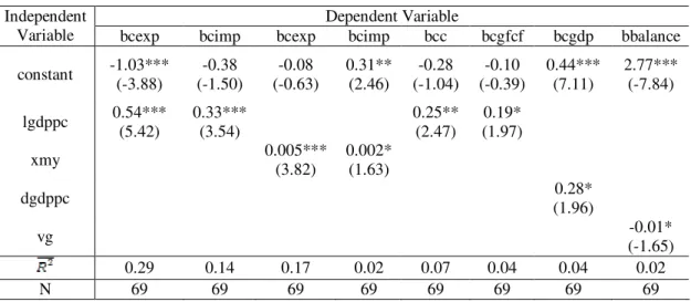
4.4. Some regression analysis
In this section we assess some potential linkages between business cycle
synchronization and other related relevant economic variables. For this purpose, we
have considered the pooled sample of 69 country observations: 15 for the sub-period
1970-1992; 27 for the sub-period 1993-1998; and finally, the remaining 27 that cover
the sub-period 1999-2009. We report in Table 9 the main results of this analysis.
Table 9 – Regression analysis
Dependent Variable
Independent
Variable
bcexp
bcimp
bcexp
bcimp
bcc
bcgfcf
bcgdp
bbalance
constant
-1.03***
(-3.88)
-0.38
(-1.50)
-0.08
(-0.63)
0.31**
(2.46)
-0.28
(-1.04)
-0.10
(-0.39)
0.44***
(7.11)
2.77***
(-7.84)
lgdppc
0.54***
(5.42)
0.33***
(3.54)
0.25**
(2.47)
0.19*
(1.97)
xmy
0.005***
(3.82)
0.002*
(1.63)
dgdppc
0.28*
(1.96)
vg
-0.01*
(-1.65)
0.29
0.14
0.17
0.02
0.07
0.04
0.04
0.02
N
69
69
69
69
69
69
69
69
***,**,* denote significance respectively at 1%, 5%, and 10%. t-statistics are in brackets.
Note:
bcexp
: Exports Business Cycle Synchronisation;
bcimp
: Imports Business Cycle Synchronisation;
bcc
: Private
Consumption Business Cycle Synchronisation;
bcgfcf
: Gross Fixed Capital Formation Business Cycle
Synchronisation;
bcgdp
: GDP Business Cycle Synchronisation;
bbalance
: Budget Balance (in percentage of GDP);
lgdppc
: Logarithm of GDP
per capita
;
xmy
: Trade-to-GDP ratio or trade openness ratio;
dgdppc
: GDP
per capita
deviation (relative to average);
vg
: Volatility of cyclical components of government spending;
According to the results we can conclude that the higher a country’s national
wealth, proxied by per capita GPD, the higher will be its exports, imports, private
degree of openness or integration in the world economy. Indeed, higher trade openness
ratios imply better business cycle synchronization in the above mentioned components.
3This analysis allows us to also to highlight an interesting outcome based on the
relation between the budget balance and the volatility of the cyclical component of
government spending. Thus, an increase in the volatility of this component of
aggregated demand reduces the budget balance (increases the budget deficit).
5. Conclusion
As argued in the literature, the stabilization costs of joining a monetary union is
a decreasing function of the correlation between the cyclical output of the member
country and the cyclical output of the union as a whole. In this context, and in the case
of the euro area, we were able to corroborate the existence of strong business cycle
correlations between individual countries and the euro area aggregates, which facilitates
the implementation of the single monetary policy by the European Central Bank.
More specifically, in this paper we have analyzed business cycle synchronization
in the EU, using annual data for the period 1970-2009. In particular we looked at
business cycle synchronization of both GDP and of the aggregate demand components.
The results that we obtained show that the level of business cycle
synchronization for the 27 EU countries has increased between 1970 and 2009, in line
with Furceri and Karras (2008). Notably, it has been higher after the introduction of the
single currency. In the most recent sub-period, we see that some of the new Member
States (Cyprus, Latvia and Slovenia) already present business cycle synchronization
similar to that of some EU-15, namely comparing to Greece and Portugal.
We also compare the peaks and troughs that we uncover with the ones reported
by the CEPR Euro Area Cycle Dating Committee, concluding that the downturns
identified by the committee are very close to the peaks and troughs that we computed
for the cyclical component of GDP (using the HP filter).
In addition, we have considered each aggregated demand sub-component,
computing for each of them the respective level of business cycle synchronization, the
volatility of its cyclical component and the corresponding respective total valued added
shares. Although private consumption is, on average, the biggest component of GDP, in
3
general and on average, external demand tends to be a more important determinant for
GDP business cycle synchronization.
Another interesting issue is the rapid growth of average share of exports in GDP
between 1970 and 2009. This evolution may be explained by a higher level of market
integration and the introduction of the single currency, which naturally facilitated intra
EU trade. Indeed, higher trade openness ratios imply better business cycle
synchronization in the imports and exports components.
References
Afonso, A. and Furceri, D. (2009). “Sectoral Business Cycle Synchronization in the
European Union”,
Economics Bulletin
, 29 (4), 2996-3014.
Angeloni, I., and Dedola, L. (1999). “From the ERM to the Euro: New Evidence on
Economic and Policy Convergence Among EU Countries”, European Central Bank
Working Paper N. 4.
Artis, M.; Marcelino, M. and Proietti, T. (2004). “Characterizing the Business Cycle for
Accession Countries,” CEPR Discussion Paper N. 4457.
Camacho, M., Perez-Quiros, G., Saiz, L. (2006). ”Are European Business Cycles Close
Enough to Be Just One?”,
Journal of Economic Dynamics and Control
, 30,
1687-1706.
Canova, F. (1998). “Detrending and business cycle facts”,
Journal of Monetary
Economics
, 41 (3), 475-512.
Clark, T. and Van Wincoop, E. (2001). “Borders and business cycles”,
Journal of
International Economics
55, 59-85.
Crowley, P. (2008). “One money, several cycles? Evaluation of European business
cycles using model-based cluster analysis”. Bank of Finland Research Discussion
Papers 3.
Fatás, A. (1997). “EMU: countries or regions: lessons from the EMS experience,”
European Economic Review
41, 743-751.
Furceri, D. and Karras, G. (2008). ”Business Cycle Synchronization in the EMU”,
Applied Economics
40, 1491-1501.
Gayer, C. (2007), "A fresh look at business cycles synchronization in the euro area",
European Economy, Economic Papers Number 287.
Giannone, D., Lenza, M. and Reichlin, L. (2008). “Business cycles in the euro area”,
Hodrick, R. and Prescott, E. (1980). “Postwar U.S. Business Cycles: An Empirical
Investigations”, Discussion Paper N. 451, Carnegie Mellon University.
Inklaar, R., Haan, J. (2001). ”Is there really a European Business Cycle? A Comment”,
Oxford Economic Papers
, 53 (2): 215-220.
Kalemli-Ozcan, S. and Papaioannou, E. (2010). “This Time Is Different: Financial
Integration and the 2007 Crisis”, mimeo, November.
Kenen, R. (1969). “The theory of optimum currency area: an eclectic view,” in: R.
Mundell and A. Swoboda, (eds.),
Monetary problems of the international economy
,
Chicago, Univeristy of Chicago Press.
Korhonen, I. (2003). ”Some Empirical Tests on the Integration of Economic Activity
between the Euro Area and the Accession Countries: A note.”
Economics of
Transition
, 11, 1-20.
Lopes, A. and Pina, A. (2008). “Business Cycles, Core and Periphery in Monetary
Unions: Comparing Europe and North America”, Department of Economics,
ISEG-UTL, Working Paper nº 07/2008/DE/UECE.
McKinnon, R. (1963). “Optimum currency areas,” American Economic Review 53,
717-725.
Mink, M., Jacobs, J., Haan, J. (2007), Measuring Synchronicity and Co-movement of
Business Cycles with an Application to the Euro Area. CESifo Working Paper No.
2112, October.
Mundell, R. (1961) “A theory of optimum currency areas,”
American Economic Review
82, 942-963.
Peiró, A. (2004). “Are Business Cycle Asymmetric? Some European Evidence”,
Applied Economics
36, 335-342.
Rose, A. and Engel, C. (2002). “Currency unions and international integration,”
Journal
of Money, Credit and Banking
34, 1067-1089.
Wynne, M. and Koo, J. (2000). “Business cycles under monetary union: a comparison
Annex – Data
Original series (from AMECO) 1/
AMECO code
GDP, current market prices
1.0.0.0.UVGD
Y
GDP, 2000 market prices
1.1.0.0.OVGD
GDP Price deflator, 2000 = 100.
3.1.0.0.PVGD
Private final consumption expenditure at current prices
1.0.0.0.UCPH
C
Private final consumption expenditure at 2000 prices
1.1.0.0.OCPH
Price deflator private final consumption expenditure
3.1.0.0.PCPH
Gross fixed capital formation at current prices; total economy
1.0.0.0.UIGT
I
Gross fixed capital formation at 2000 prices; total economy
1.1.0.0.OIGT
Price deflator gross fixed capital formation; total economy
3.1.0.0.PIGT
Gross capital formation; general government at current prices
1.0.0.0.UIGG0
Gross fixed capital formation at current prices; private sector
1.0.0.0.UIGP
Final consumption expenditure of general government at current prices 1.0.0.0.UCTG
G
Exports of goods and services at current prices (National accounts)
1.0.0.0.UXGS
X
Exports of goods and services at 2000 prices
1.1.0.0.OXGS
Price deflator exports of goods and services
3.1.0.0.PXGS
Imports of goods and services at current prices (National accounts)
1.0.0.0.UMGS
M
Imports of goods and services at 2000 prices
1.1.0.0.OMGS
Price deflator imports of goods and services
3.1.0.0.PMGS
Net exports of goods and services at current prices (National accounts) 1.0.0.0.UBGS
X-M
Domestic demand excluding stocks at current prices
1.0.0.0.UUNF
Domestic demand including stocks at current prices
1.0.0.0.UUNT
Change in inventories
1.0.0.0.UUNT -
1.0.0.0.UUNF
CHI
1/ European Commission
Annual Macro-economic Database
(AMECO).
Y=C+I+G+(X-M)+CHI.
Appendix 1 - Business cycle synchronization (vis-à-vis EU15, HP filter
,
=100
)
Table A1.1 – GDP Business cycle synchronisation (vis-à-vis EU15)
Business Cycle Synchronization Volatility of the cyclical component
1970-1992 1993-1998 1999-2009 1970-2009 1970-1992 1993-1998 1999-2009 1970-2009
Austria 0.793*** 0.619* 0.899*** 0.861*** 2.039 0.709 4.043 2.625
Belgium 0.883*** 0.516 0.958*** 0.916*** 2.900 1.324 4.152 3.222
Bulgaria 0.349 0.583** 0.534*** 1.554 1.351 1.405
Cyprus 0.275 0.799*** 0.565*** 0.160 0.152 0.150
Czech Republic -0.395 0.706*** 0.454*** 60.991 88.901 89.064
Denmark -0.129 0.183 0.952*** 0.515*** 17.427 19.101 30.317 21.594
Estonia -0.134 0.822*** 0.712*** 3.328 10.455 8.493
Finland 0.167 0.244 0.994*** 0.632*** 3.178 3.291 4.386 3.887
France 0.9*** 0.898*** 0.975*** 0.918*** 16.308 6.812 20.859 18.482
Germany 0.61*** 0.213 0.914*** 0.619*** 45.262 19.157 39.624 40.192
Greece 0.67*** 0.451 0.72*** 0.692*** 2.785 0.304 2.808 2.677
Hungary 0.491 0.793*** 0.837*** 154.828 536.725 479.879
Ireland 0.125 0.139 0.919*** 0.751*** 0.806 1.261 6.184 3.570
Italy 0.837*** 0.235 0.969*** 0.911*** 14.258 5.756 22.989 16.696
Latvia 0.14 0.874*** 0.763*** 0.286 0.649 0.724
Lithuania 0.018 0.826*** 0.778*** 3.339 5.141 5.783
Luxembourg 0.922*** 0.277 0.958*** 0.894*** 0.368 0.516 0.739 0.528
Malta 0.159 0.622** 0.494*** 0.037 0.097 0.076
Netherlands 0.836*** 0.287 0.862*** 0.849*** 4.076 3.082 9.947 6.301
Poland 0.06 0.279 0.237* 16.935 19.705 21.047
Portugal 0.717*** 0.21 0.769*** 0.708*** 2.604 1.412 2.357 2.472
Romania -0.386 0.53** 0.3** 4.734 5.277 5.509
Slovakia -0.127 0.535** 0.319** 0.503 1.752 1.454
Slovenia 0.179 0.904*** 0.715*** 0.251 0.724 0.746
Spain 0.823*** 0.556 0.967*** 0.897*** 11.179 3.169 15.454 12.629
Sweden 0.326* 0.453 0.944*** 0.736*** 31.963 25.707 62.279 45.573
UK 0.416** 0.397 0.951*** 0.717*** 16.767 7.263 22.462 17.984
Minimum -0.129 -0.395 0.279 0.237* 0.368 0.037 0.097 0.076
Maximum 0.922*** 0.898*** 0.994*** 0.918*** 45.262 154.828 536.725 479.879
Average 0.593 0.234 0.816 0.679 11.461 12.808 34.057 30.102
Average EU15 0.593 0.378 0.917 0.774 11.461 6.591 16.573 13.229