www.ocean-sci.net/12/577/2016/ doi:10.5194/os-12-577-2016
© Author(s) 2016. CC Attribution 3.0 License.
Design and validation of MEDRYS, a Mediterranean Sea
reanalysis over the period 1992–2013
Mathieu Hamon1, Jonathan Beuvier1,2, Samuel Somot2, Jean-Michel Lellouche1, Eric Greiner3, Gabriel Jordà4, Marie-Noëlle Bouin2, Thomas Arsouze5, Karine Béranger6, Florence Sevault2, Clotilde Dubois1, Marie Drevillon1, and Yann Drillet1
1Mercator Océan, 10 rue Hermès, 31520 Ramonville-Saint-Agne, France 2Météo France, 42 av. Gaspard Coriolis, 31057 Toulouse CEDEX, France 3CLS, 11 rue Hermès, 31520 Ramonville-Saint-Agne, France
4Department of Ecology and Marine Resources, IMEDEA (CSIC-UIB),
Institut Mediterrani d’Estudis Avançats, Esporles (Illes Balears), Spain
5LMD, école Polytechnique, 91128 Palaiseau CEDEX, France 6LTHE, rue de la Piscine, 38400 Saint-Martin d’Hère, France
Correspondence to:Jonathan Beuvier ([email protected]) Received: 24 July 2015 – Published in Ocean Sci. Discuss.: 18 August 2015 Revised: 14 December 2015 – Accepted: 1 April 2016 – Published: 22 April 2016
Abstract. The French research community in the Mediter-ranean Sea modeling and the French operational ocean fore-casting center Mercator Océan have gathered their skill and expertise in physical oceanography, ocean modeling, atmospheric forcings and data assimilation to carry out a MEDiterranean sea ReanalYsiS (MEDRYS) at high reso-lution for the period 1992–2013. The ocean model used is NEMOMED12, a Mediterranean configuration of NEMO with a 1/12◦(∼7 km) horizontal resolution and 75 vertical
z levels with partial steps. At the surface, it is forced by a new atmospheric-forcing data set (ALDERA), coming from a dynamical downscaling of the ERA-Interim atmospheric reanalysis by the regional climate model ALADIN-Climate with a 12 km horizontal and 3 h temporal resolutions. This configuration is used to carry a 34-year hindcast simulation over the period 1979–2013 (NM12-FREE), which is the ini-tial state of the reanalysis in October 1992. MEDRYS uses the existing Mercator Océan data assimilation system SAM2 that is based on a reduced-order Kalman filter with a three-dimensional (3-D) multivariate modal decomposition of the forecast error. Altimeter data, satellite sea surface tempera-ture (SST) and temperatempera-ture and salinity vertical profiles are jointly assimilated. This paper describes the configuration we used to perform MEDRYS. We then validate the skills of the data assimilation system. It is shown that the data
as-similation restores a good average temperature and salinity at intermediate layers compared to the hindcast. No particular biases are identified in the bottom layers. However, the re-analysis shows slight positive biases of 0.02 psu and 0.15◦C
above 150 m depth. In the validation stage, it is also shown that the assimilation allows one to better reproduce water, heat and salt transports through the Strait of Gibraltar. Fi-nally, the ability of the reanalysis to represent the sea surface high-frequency variability is shown.
1 Introduction
The Mediterranean Sea is a semi-enclosed sea located be-tween 5.5◦W and 36◦E and between 30 and 46◦N. It is
con-nected to the Atlantic Ocean through the Strait of Gibral-tar and to the Black Sea through the Dardanelles and the Bosphorus straits. The surrounding orography tends to gen-erate cold and dry regional northern winds over the Mediter-ranean Sea. This leads to strong heat and freshwater losses by evaporation and latent heat transfer. The heat loss is esti-mated around 5 W m−2 (MacDonald et al., 1994) while the
freshwater loss is about 0.6 m year−1(Mariotti et al., 2008).
Strait of Gibraltar while it is estimated that only about 10 % of the net water flux is balanced with river runoff (Struglia et al., 2004).
In a climate change context, the Mediterranean area is con-sidered as a hot spot and shows an increase in the temperature and precipitation interannual variability, and a strong warm-ing and drywarm-ing (Giorgi et al., 2006). The vulnerability of the population is likely to increase with a higher probability of events occurring that lead to floods and droughts, which are among the most devastating natural hazards. In this context, it is necessary to simulate the water cycle over the Mediter-ranean basin (Drobinski et al., 2013) and to understand how it will impact water resources. We must improve our under-standing of the variability of the water cycle, from extreme events to the seasonal and interannual scales. In addition to the socioeconomic motivations and from a strictly physical point of view, the specific configuration of the basin also per-mits the study of a wide variety of dynamical oceanic pro-cesses. For example, the Mediterranean Sea has been found to have a dominant mesoscale circulation component (Robin-son et al., 1987; Ayoub et al., 1998; Hamad et al., 2005; Fernandez et al., 2005) in addition to a thermohaline circu-lation similar to the world ocean (Wüst, 1961; Robinson et al., 2001). The Mediterranean eddy field also shows semi-permanent structures (Rhodes and South Adriatic gyres for example) that define the general circulation in the basin. Modeling the different timescales and spatial scales of this circulation is still challenging because, for example, of ap-proximations and uncertainties on nonlinear dynamical bal-ance, atmospheric forcing or the bathymetry (Sorgente et al., 2011; Pinardi et al., 2013).
The ocean reanalysis is a reconstruction technique that al-lows for the production of a consistent four-dimensional (4-D) estimate of a physical field from observations and nu-merical modeling simulation. Observations are used to con-strain the model trajectory to be as close as possible to the “real” state of the ocean. Ocean reanalyses are thus refer-ence products that help to improve our knowledge of the ocean variability at various space scales and timescales. Sev-eral techniques have been used in the past to produce large-scale reanalysis but regional reanalyses are challenging be-cause observational data sets are scarcer and the use of high-resolution model requires one to adequately represent fluxes through the air–sea interface. This is even more important in the Mediterranean Sea due to the complex orography. Many small-size islands and a particularly complex coastline limit the low-level air flow, channeling potentially strong and re-curring regional winds (Mistral, Tramontane, Bora, Etesian, Sirocco; Herrmann et al., 2011). The role of the spatial res-olution of the forcing has been highlighted as a key aspect of the representation of Mediterranean Sea phenomena such as local winds (Sotillo et al., 2005; Ruti et al., 2007; Her-rmann et al., 2011; Lebeaupin Brossier et al., 2012), open-sea deep convection (Herrmann and Somot, 2008; Béranger et al., 2010), shelf-cascading (Dufau-Julliand et al., 2004;
Langlais et al., 2009), coastal upwelling (Estournel et al., 2009; Casella et al., 2011), permanent circulation features (Estournel et al., 2003; Ourmières et al., 2011) or intermit-tent eddies (Marullo et al., 2003; Ciappa, 2009; Rubio et al., 2009). The infra-diurnal temporal resolution of the forc-ing has also been identified as necessary to represent key phenomena such as large salinity anomalies following in-tense rainfall events (Lebeaupin Brossier et al., 2012) or the sea surface temperature (SST) diurnal cycle (Lebeaupin Brossier et al., 2011, 2014). Other studies demonstrated the importance of the good representation of the atmospheric synoptic chronology linked with the so-called weather pat-terns or weather regimes (Josey et al., 2011; Papadopoulos et al., 2012; Durrieu de Madron et al., 2013) or with the passage of Mediterranean storms associated with strong air– sea exchanges (Herrmann and Somot, 2008; Herrmann et al., 2010). At a longer timescale, interannual to decadal vari-ability of the atmospheric forcings (water or heat fluxes) is known to dominate the climate variability of the deep wa-ter mass formation in both basins of the Mediwa-terranean Sea (Beuvier et al., 2010; Herrmann et al., 2010; L’Heveder et al., 2013), leading sometimes to exceptional decadal events such as the Eastern Mediterranean Transient (Roether et al., 2007) or the Western Mediterranean Transition (Schroeder et al., 2008).
The first regional Mediterranean reanalyses have been re-cently produced over the 1985–2007 period by Adani et al. (2011), using a reduced-order optimal interpolation and a 3-D variational scheme. Their OPA ocean model (Océan PArallélisé, Madec et al. 1997) on a 1/16◦regular horizontal
grid (Tonani et al., 2008) is forced by daily atmospheric fields from the European Center Medium-Range Weather Fore-cast (ECMWF) with bulk parameterizations and a monthly precipitation climatology. They used the reanalysis ERA-15 for the 1985–1992 period and then the operational analyses for the 1993–2007 period. We note thus several successive changes in the atmospheric forcing, in particular during the 1993–2007 period, for which the resolution of the ECMWF analyses has progressively increased in several steps from about 100 to 25 km. Such changes suggest that temporal con-tinuity and coherence in atmospheric forcing are not guaran-teed. However, the first results of these reanalyses pointed out, for example, that such products allow one to better sim-ulate the AW salinity inflow, the sea surface height variability and current–jet pathways.
around 1/12◦ over the world ocean. Within our numerical
domain, the ORCA grid has a horizontal resolution rang-ing between 6 and 7.5 km. Note that this spatial resolution is similar to the 1/16◦regular horizontal grid used in Adani et al. (2011). MEDRYS differs in that it uses of a reduced-order Kalman filter in the assimilation scheme from the French op-erational oceanography center Mercator Océan and the long-term 12 km high-resolution fields of the atmospheric forc-ing called ALDERA. Even if we cannot overcome other ho-mogeneity issues resulting from the coverage of the observ-ing network (applyobserv-ing in both MEDRYS and ALDERA), we pay a special attention to the consistency of the atmospheric forcing (same resolution, same model physics) in order to reduce as much as possible the sources of inhomogeneity in MEDRYS. This reanalysis then contributes to better describe the interannual to decadal variability of the Mediterranean circulation and trends
In the current paper, we first present the configuration of the reanalysis MEDRYS and the twin hindcast NM12-FREE in Sect. 2. Then, Sect. 3 presents validation diagnostics and some scientific assessments. Finally, discussions and conclu-sion are conducted in Sect. 4.
2 Experimental setup
Two twin simulations have been produced: MEDRYS, a Mediterranean reanalysis covering the 1992–2013 period with data assimilation and its associated free-run NM12-FREE, a 34-year hindcast simulation covering the 1979– 2013 period without assimilation. Both simulations use the same ocean model configuration, NEMOMED12, described in Sect. 2.1 and the high-resolution atmospheric-forcing ALDERA, presented in Sect. 2.3. Specific setups concern-ing data assimilation in the reanalysis are then presented in Sect. 2.4 and 2.5.
2.1 Ocean model configuration: NEMOMED12 We use the ocean general circulation model NEMO (Madec and the NEMO team, 2008) in a regional configuration of the Mediterranean Sea called NEMOMED12 (Lebeaupin Brossier et al., 2011, 2012; Beuvier et al., 2012a, b; hereafter NM12). The development of NM12 is made in the continu-ity of the evolution of the French modeling of the Mediter-ranean Sea, following OPAMED16 (Béranger et al., 2005), OPAMED8 (Somot et al., 2006) and NEMOMED8 (Beuvier et al., 2010). More details concerning the physical parameter-izations and the boundary conditions in NM12 can be found in Beuvier et al. (2012a).
The NM12 configuration covers the whole Mediterranean Sea and a buffer zone including a part of the Atlantic basin, but not the Black Sea. The horizontal resolution is 1/12◦and
corresponds to a varying grid cell size between 6 and 7.5 km (the distance between two points varying with the cosine of
the latitude). NM12 has 75 vertical stretchedzlevels (from
1z=1 m at the surface to1z=135 m at the bottom, with 43 levels in the first 1000 m) in a partial step configuration. The bottom layer thickness is varying to fit the bathymetry (Mercator-LEGOS version 10 bathymetry at 1/120◦ resolu-tion). The no-slip boundary condition is used and the con-servation of the model volume is assumed. The mean tidal effect of the quadratic bottom friction formulation computed from a tidal model (Lyard et al., 2006) has been taken into account, leading to significant additional bottom friction in the Strait of Gibraltar, Channel of Sicily, Gulf of Gabès and the northern Adriatic sub-basin. As a lateral boundary con-ditions and in order to represent the exchanges with the At-lantic Ocean, a buffer zone is used: from 11 to 7.5◦W, 3-D
temperature and salinity, as well as the sea surface height (SSH) fields are relaxed toward ORAS4 global ocean reanal-ysis monthly fields (Balmaseda et al., 2013), produced by the ECMWF. For temperature and salinity, the restoring term in the buffer zone is weak west of the Cadiz and Gibraltar ar-eas and incrar-eases westwards. As the Mediterranean Sea is an evaporation basin, the model volume is conserved through the damping of the SSH in the buffer zone toward prescribed SSH anomalies with a very strong restoring. The SSH from ORAS4 is set in the Atlantic according to a strong damping with a very small characteristic timescale (τ =2 s).
We use the climatological averages of the interannual data set of Ludwig et al. (2009) to compute monthly runoff val-ues, split in two parts (Beuvier et al., 2012a). The 33 main rivers of the NM12 domain are added as precipitation at mouth points (29 in the Mediterranean Sea and 4 in the buffer zone). As the Ludwig et al. (2009) data set consists in 239 mouth points, the inputs of the 210 other rivers in the Mediterranean basin are gathered as a coastal runoff in each subbasin (following the same dividing as in Ludwig et al., 2009). Until 2000, we use the interannual values from Lud-wig et al. (2009) and then the climatological average repre-senting the 1960–2000 period. The Black Sea, not included NM12, is taken into account with a monthly average one layer net flow across the Marmara Sea and the Dardanelles Strait. We assume that the flow is a freshwater flux (Beuvier et al., 2012a). Until 1997, we use the interannual values from Stanev et Peneva (2002) and then the climatological average representing the 1960–1997 period.
2.2 Simulations: NM12-FREE and MEDRYS
Rixen et al. (2005), the filtered interannual product is used in order to reduce the impact of large spatiotemporal gaps in the data distribution. In the buffer zone, potential temper-ature and salinity are initialized from ORAS4 global ocean reanalysis fields in order to maintain consistency with the re-laxation. In the initial condition fields, a linear transition be-tween 7.5 and 6◦W is applied between the ORAS4 and the
MedAtlas fields. MEDRYS starts from the state of NM12-FREE in October 1992 and ends in June 2013.
2.3 Atmospheric forcing: ALDERA
The most recent long-term hindcast simulations using the NEMOMED12 ocean model (Beuvier et al., 2012b; Soto-Navarro et al., 2014; Palmiéri et al., 2015) were driven by the ARPERA2 data set (Herrmann et al., 2010). This forcing was obtained by a dynamical downscaling using the stretched-grid Regional Climate Model (RCM) ARPEGE-Climate and a spectral nudging technique. ARPERA2 covers the period 1958–2013 with a daily temporal resolution and a 50 km spa-tial resolution over the Mediterranean Sea. It may include temporal inhomogeneity especially in 2001 when the large-scale driving fields change from ERA-40 to ECMWF analy-sis.
In order to overcome the main deficiencies of the ARPERA2 data set (relatively coarse spatial and temporal resolution, temporal homogeneity issue), we use a new forc-ing data set for MEDRYS and NM12-FREE. This data set (called hereafter ALDERA) is based on a dynamical down-scaling of the ERA-Interim reanalysis (Dee et al., 2011) over the period 1979–2013 by the RCM ALADIN-Climate (Radu et al., 2008; Colin et al., 2010; Herrmann et al., 2011). The dynamical downscaling technique is commonly used to over-come the lack of atmospheric regional reanalysis over sea and to improve locally the resolution of the air–sea forc-ing in areas dominated by small-scale atmospheric patterns such as the Mediterranean Sea (Sotillo et al., 2005; Her-rmann and Somot, 2008; Beuvier et al., 2010; HerHer-rmann et al., 2010, 2011; Josey et al., 2011; Beuvier et al., 2012a; Lebeaupin-Brossier et al., 2012; Solé et al., 2012; Vervatis et al., 2013; Auger et al., 2014; Harzallah et al., 2014). In ALDERA, we use the version 5 of ALADIN-Climate, first described in Colin et al. (2010). For the model defini-tion, we used a Lambert conformal projection for the pan-Mediterranean area at the horizontal resolution of 12 km cen-tered at 14◦E, 43◦N with 405 grid points in longitude and
261 grid points in latitude excluding the coupling zone. The model version has 31 vertical levels. The time step used is 600 s. This geographical setup allows the Med-CORDEX of-ficial area (Ruti et al., 2015; www.medcordex.eu) to be fully included in the model central zone. In this configuration, the RCM is driven at its lateral boundary by the ERA-Interim reanalysis (T255, 80 km at its full resolution; Dee et al., 2011; http://www.ecmwf.int/en/research/climate-reanalysis/ era-interim), which is updated every 6 h. The ERA-Interim
data assimilation system uses a 2006 release of the Inte-grated Forecasting System, which contains many improve-ments both in the forecasting model and analysis method-ology relative to ERA-40. Before starting this simulation, a 2-year long spin-up is carried out allowing the land water content to reach its equilibrium. Land surface parameters and aerosol concentrations are updated every month following a climatological seasonal cycle coming from observations. The sea surface temperatures and the sea ice limit are updated every month with a seasonal and interannual variability us-ing the same SST and sea ice analyses as the one used to drive the ERA-Interim reanalysis (Dee et al., 2011). As at-mospheric reanalyses constitute today the best knowledge of the 4-D dynamic of the atmosphere available over the last decades, such a simulation is often called “perfect-boundary simulation” or “poor-man regional reanalysis”.
ALDERA is available at a 12 km spatial resolution and a 3 h temporal resolution over the whole Mediterranean Sea, Black Sea and near-Atlantic Ocean. It includes a rep-resentation of the effect of the aerosols on the longwave and shortwave radiations and uses the same bulk formula as in ARPERA2 (Louis, 1979) to compute the turbulent fluxes (sensible heat, latent heat and momentum fluxes). All variables required to drive regional ocean models us-ing bulk formula or flux formulation are available. For the NEMOMED12 configuration (both NM12-FREE and MEDRYS) reanalysis, the various fluxes have been inter-polated every 3 h on the NEMOMED12 grid using a con-servative interpolation scheme. NEMOMED12 receives heat fluxes (total and solar for the light penetration), net freshwa-ter fluxes (evaporation and precipitation) and wind stresses every 3 h. A retroaction term towards the same SST fields as the one seen by ALADIN-Climate is added in the heat flux, following the method of Barnier et al. (1995), with a retroac-tion coefficient of−40 W m−2K−1. The total heat flux,
in-cluding the retroaction term, has been stored when running the hindcast NM12-FREE and is used to force MEDRYS, ensuring thus that both simulations have exactly the same at-mospheric forcing.
No sea surface salinity (SSS) damping is used but a 2-D-smoothed monthly climatological freshwater flux correc-tion is added, following the same method as in Beuvier et al. (2012a), but with the 2-D spatial variability kept: these monthly 2-D fields have been computed by averaging the SSS relaxation term through a previous companion simula-tion with NEMOMED12 and the same atmospheric forcing, and then filtered at the resolution of 1◦by a spatial averaging.
The surface freshwater budget is thus balanced without alter-ing the spatial and temporal variations of the freshwater flux as well as the SSS. This correction term is added to the water fluxes coming from the atmospheric fields and from the river and Black Sea runoff.
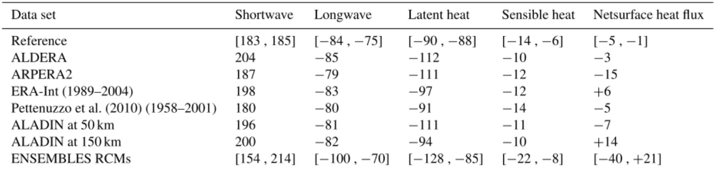
Table 1.Mediterranean Sea-averaged and temporal-averaged values of the various terms of the sea surface heat budget (W m2). Values are computed over the 1985–2004 period except for when indicated. The reference comes from Sevault et al. (2014). The so-called ENSEMBLES RCMs is an ensemble of 15 runs carried out with state-of-the-art RCMs during the EU project ENSEMBLES at 25 km, driven by the ERA-40 reanalysis over the 1958–2001 period (see Sanchez-Gomez et al., 2011).
Data set Shortwave Longwave Latent heat Sensible heat Netsurface heat flux
Reference [183 , 185] [−84 ,−75] [−90 ,−88] [−14 ,−6] [−5 ,−1]
ALDERA 204 −85 −112 −10 −3
ARPERA2 187 −79 −111 −12 −15
ERA-Int (1989–2004) 198 −83 −97 −12 +6 Pettenuzzo et al. (2010) (1958–2001) 180 −80 −91 −14 −5 ALADIN at 50 km 196 −81 −111 −11 −7 ALADIN at 150 km 200 −82 −94 −10 +14 ENSEMBLES RCMs [154 , 214] [−100 ,−70] [−128 ,−85] [−22 ,−8] [−40 ,+21]
ALDERA in order to illustrate the small-scale features of the 12 km resolution model with respect to lower resolution models (see later comments for Tables 1 and 2 and Figs. 1 and 2).
2.3.1 Long-term Mediterranean Sea surface heat and water budgets
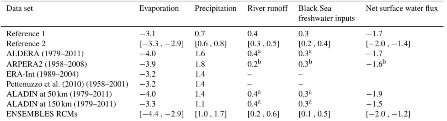
Tables 1 and 2 compares the spatially and temporally aver-aged values of the Mediterranean Sea surface heat and wa-ter budget wa-terms of the ALDERA forcing with past stud-ies and observed-based references (flux are positive down-ward in W m−2 and mm day−1). ALDERA shows values
within the range of the references for the net heat and wa-ter surface fluxes, respectively, with −3 W m−2 over the
1985–2004 period (−4 W m−2 over the 1979–2012 period)
and −1.69 mm day−1 (1979–2011). Over the 20-year
pe-riod considered, ALDERA shows compensating errors be-tween an overestimated shortwave and an overestimated la-tent heat loss when compared to the observation-based esti-mates (Sevault et al., 2014). Both values are in equilibrium with the heat and water transports at the Strait of Gibral-tar (see Sect. 3.2.6). However, some individual terms show biases. This is especially true for the shortwave radiation, the latent heat flux (and consequently the evaporation) and the precipitation averaged over the sea surface. Note that ALDERA and ARPERA2 show very similar results, which is expected as they share most of their physical parameteri-zations. This also means that increasing the spatial resolution in the RCMs does not fundamentally change the mean biases at least from 50 to 12 km. This is confirmed when comparing ALDERA to the ALADIN-Climate simulation at 50 km res-olution. ALADIN-Climate ran at 150 km is however closer to ERA-Interim with a weaker latent heat loss. Note that the Pettenuzzo et al. (2010) data set also achieves the Mediter-ranean sea heat budget balance but with lower values both for shortwave radiation and the latent heat loss. When com-pared to the ENSEMBLES RCMs used in the last published multi-model intercomparison study with Atmosphere RCM
(Sanchez-Gomez et al., 2011), ALDERA always fits inside the uncertainty range.
2.3.2 Interannual variability and trends
At the basin scale, the interannual variability of the vari-ous terms of the Mediterranean Sea heat budget can also be evaluated for the period 1985–2004 of the reference data set of Table 1 (Sevault et al., 2014). For example, for the basin-averaged net shortwave radiation flux, the interannual standard deviation in ALDERA (1.6 W m−2) is
underesti-mated with respect to International Satellite Cloud Clima-tology Project (ISCCP; http://isccp.giss.nasa.gov/) observa-tions (2.8 W m−2)whereas the interannual temporal
corre-lation is equal to 0.84. For the latent heat loss, the 1985– 2004 interannual standard deviation is equal to 5.6 W m−2in ALDERA within the range of the observations (4.7 W m−2 for the NOCS data set – National Oceanography Centre Southampton – and 6.7 W m−2for the OAFlux data set –
Ob-jectively Analyzed air–sea Fluxes) and the interannual tem-poral correlation is good (0.83 with NOCS and 0.81 with OAFlux). Interannual standard deviations are lower for the net longwave radiation flux (1.2 W m−2 in ALDERA), and
for the sensible heat loss (1.3 W m−2in ALDERA) and the
various observation-based estimates disagree (not shown). Trends in the surface forcing are relevant in long-term simulations as they can induce long-term trends in the wa-ter mass characwa-teristics. Concerning the surface heat flux terms in ALDERA, only the trend in latent heat flux is sig-nificant with an increase in the heat loss by the sea equal to+4.1 W m−2decade−1 over the 1979–2012 period. This
Table 2.Same as Table 1 but for the Mediterranean Sea surface water budget terms (mm day−1). The reference 1 comes from Sanchez-Gomez et al. (2011) and the reference 2 from Dubois et al. (2010). The reference values do not always cover a common period.
Data set Evaporation Precipitation River runoff Black Sea Net surface water flux freshwater inputs
Reference 1 −3.1 0.7 0.4 0.3 −1.7
Reference 2 [−3.3 ,−2.9] [0.6 , 0.8] [0.3 , 0.5] [0.2 , 0.4] [−2.0 ,−1.4] ALDERA (1979–2011) −4.0 1.6 0.4a 0.3a −1.7 ARPERA2 (1958–2008) −3.9 1.8 0.2b 0.3b −1.6b ERA-Int (1989–2004) −3.2 1.4 – –
Pettenuzzo et al. (2010) (1958–2001) −3.2 1.4 – –
ALADIN at 50 km (1979–2011) −4.0 1.4 0.4a 0.3a −1.9 ALADIN at 150 km (1979–2011) −3.3 1.1 0.4a 0.3a −1.5 ENSEMBLES RCMs [−4.4 ,−2.9] [1.0 , 1.7] [0.2 , 0.6] [0.1 , 0.5] [−2.0 ,−1.2]
aThe ALDERA atmospheric forcing is here completed by the river runoff and Black Sea freshwater inputs coming respectively from Ludwig et al. (2009) and Stanev and Peneva (2002) as used in Beuvier et al. (2012b) and in MEDRYS.bThe ARPERA2 atmosphere forcing is here completed by the river runoff and Black Sea freshwater inputs coming respectively from Ludwig et al. (2009) and Stanev and Peneva (2002) as used in the Herrmann et al. (2010) paper.
2.3.3 Illustration of the small-scale features in the ALDERA forcing
Over the Mediterranean Sea, the added-value of high-resolution models has been shown in particular concerning the representation of the heat and water budget terms (El-guindi et al., 2011; Josey et al., 2011), of wind field espe-cially close to the coast and islands (Sotillo et al., 2005; Ruti et al., 2007; Herrmann and Somot, 2008; Langlais et al., 2009; Herrmann et al., 2011; Vrac et al., 2012) and of the events of strong air–sea fluxes (Herrmann and Somot, 2008; Béranger et al., 2010; Lebeaupin-Brossier et al., 2012). Dy-namical downscaling of reanalyses have therefore been used to force long-term hindcast simulations (Beuvier et al., 2010, 2012; Herrmann et al., 2010; Solé et al., 2012; Vervatis et al., 2013; Auger et al., 2014; Harzallah et al., 2014). Fig-ure 1 illustrates the role of the atmospheric resolution in the representation of the wind and the latent heat flux on 14 March 2013 in the Gulf of Lions by comparing ALDERA at 12 km with ALADIN-Climate runs at lower resolution. This particular date has been selected because of the strong Mistral event in the Gulf of Lions. Increasing the resolution allows ALDERA to create small-scale features of the wind near the coast as well as the associated pattern of latent heat flux during the Mistral event. The comparison of latent heat flux at 42◦N, 5◦E also indicates that the maximum of latent
heat flux is resolution dependent. In ALADIN-12 km (the so-called ALDERA), the maximum of latent heat loss is about 900 W m−2, whereas in ALADIN-150 km, it barely reaches
500 W m−2with ALADIN-50 km being intermediate range. Figure 2 also illustrates the resolution dependency of the surface wind field but over the eastern Mediterranean basin during a Meltemi (or Etesian) event (16 August 2012). This case shows the clear shadowing effect of the Greek islands. The wind channeling at 12 km leads locally to increased wind speed, changes in wind direction and increased vorticity
in-puts for the ocean due to strong horizontal gradients. All these effects are visible at the southeastern part of Crete, an area where the Ierapetra anticyclone is formed regularly (see below). Note that the goal here is not to prove the added value of the 12 km with respect to lower resolution as in situ observations and regridding would be required for this pur-pose, but to illustrate differences between the three resolu-tions (150, 50 and 12 km) and to show ALDERA small-scale features with potential impacts on local to regional Mediter-ranean Sea circulation.
2.4 Data assimilation scheme
The data assimilation system used in MEDRYS is SAM2 (Système d’Assimilation Mercator 2nd version), which is used at Mercator Océan for operational oceanography pur-poses. The Mercator Océan monitoring and forecasting sys-tem has demonstrated its skills for the global ocean forecast (Lellouche et al., 2013) and we used it in a regional config-uration. As the main part of the assimilation scheme used in this paper is already described by Lellouche et al. (2013), we will summarize the assimilation methodology and focus on the specifications inherent to the Mediterranean configura-tion.
Figure 1. Daily average wind direction (arrows) and latent heat flux (color in W m−2) on 14 March 2013 in (a) ALADIN-150 km,(b)ALADIN-50 km and(c)ALADIN-12 km (the so-called ALDERA).
the Nth day of a given year, ocean-state anomalies com-puted from NM12-FREE within the window [N−60 days;
N+60 days] of each year are gathered and define the co-variance of the model forecast error. For the Mediterranean configuration, we computed about 900 anomaly fields from NM12-FREE for a given assimilation cycle. Compared to a global configuration, the moderate size of the domain allows us to use such a number of anomaly fields (about 300 in a global configuration) in order to statically compute an accu-rate error covariance field. Moreover, as the analysis incre-ment is a linear combination of the anomalies, a large amount of anomalies is desirable in order to better span the oceanic variability.
Figure 2. Daily average wind direction (arrows) and wind speed (color in m s−1) on 16 August 2012 in (a) ALADIN-150 km,(b)ALADIN-50 km and(c)ALADIN-12 km (the so-called ALDERA).
Mediter-ranean Sea, strong regional winds occur in areas with low bathymetry and near important straits like Gibraltar and Sicily. A significant part of SSH is then driven non-locally by the wind. Shelf surge and hydraulic control effects are typically 10 times larger in the Mediterranean Sea than in the middle of the ocean. In our regional configuration, SSH in-crements are purely statistical and derived by the covariances between SSH (the prognostic variable of the model), temper-ature and salinity implied by the ensemble of anomalies. 2.5 Observational data sets
The assimilated observations in MEDRYS consist of SST maps, along-track sea level anomaly (SLA) data and in situ temperature and salinity profiles. For each cycle, we assimilate the associated centered SST map coming from the daily NOAA Reynolds 0.25◦ product, including
vanced Very High Resolution Radiometer (AVHRR) and Ad-vanced Microwave Scanning Radiometer (AMSR) observa-tions (Reynolds et al., 2007). We assimilate SST only each 1◦to avoid correlation problem between observations. More-over, we noted a negative average bias of 0.2◦C between
the AVHRR-AMSR product and the ERA-Interim reanaly-sis SST that has been used for flux computation. For the sake of consistency between fluxes and assimilated SST in MEDRYS, we decided to add 0.2◦C to the AVHRR-AMSR
maps as a constant offset.
Along-track SLA delayed-time products, specifically re-processed for Mediterranean Sea, and distributed by AVISO (http://www.aviso.altimetry.fr) in April 2014 in the frame-work of MyOcean project, are assimilated in MEDRYS. These products include along-track filtering (low-pass fil-tered with a cutoff wavelength of 65km for the whole do-main) and along-track sub-sampling (only one point over two is retained to avoid taking into account redundant informa-tion). For these products, the reference period of the SLA is based on a 20-year (1993–2012) period. Names and abbrevi-ations used in this paper as well as the measurement period of each satellite are summarized in Table 3. The assimilation of SLA observations requires the knowledge the observation error and of a mean dynamic topography (MDT). As the sim-ulated Mediterranean Sea has a constant volume in the NM12 configuration, a volume correction term is also needed for the computation of the observation operator in MEDRYS. Con-cerning the observation error, we choose to not trust observa-tions near the coastal areas. The observation error is then ar-tificially increased within 50 km of the whole Mediterranean coast. The mean surface reference used is a hybrid product between the CNES-CLS09 MDT (Rio et al., 2011) adjusted with the data from the Gravity Field and Steady-State Ocean Circulation Explorer (GOCE) and from the Mercator Océan 1/4◦ Reanalysis GLORYS2V1(Lellouche et al., 2013)
rep-resenting the 1993–2012 period. In MEDRYS, the volume correction consists in adding a term in the SLA observation operator, representing the effect of the glacial isostatic
ad-Table 3.Name, abbreviation and period of SLA measurement for all satellite used by the assimilation process.
Satellite name Abbreviation Begin End
ERS2 e2 15 May 1995 9 Apr 2003
Topex/Poseidon tp 25 Sep 1992 24 Apr 2002 Topex/Poseidon (interleaved) tpn 16 Sep 2002 8 Oct 2005 Geosat Follow-On g2 7 Jan 2000 7 Sep 2008
Jason 1 j1 24 Apr 2002 19 Oct2008
Envisat en 9 Oct 2002 22 Oct 2010
Jason 2 j2 19 Oct 2008 now
Jason 1 (interleaved) j1n 14 Feb 2009 now Envisat (interleaved) enn 22 Oct 2010 now
Cryosat 2 c2 19 Feb 2012 now
Jason 1 Geodetic j1g 14 May 2012 now
justment (GIA) and the barystatic effect due to the mass in-take of continental ice melting. The spatial fluctuations of the GIA are applied on the MDT to compensate for the local deformation of the geoid due to the ongoing deformation of the solid Earth (Peltier et al., 2008). For the global ocean on average, the correction is about−0.3 mm year−1. In addition
we also apply a correction to compensate the mass intake of continental ice melting in the Mediterranean basin. On aver-age, the mass intake corresponds to a rise of 0.85 mm year−1. In situ temperature and salinity profiles come from the CORA4 (Cabanes et al., 2013) in situ database provided by CORIOLIS data center from the start of the reanalysis up to December 2012. For the last 6 months we used the real-time database. A check through objective quality control and a data thinning have been done on the data set in CORA4. Indeed, for each instrument, only one profile per day and within a 0.1◦ distance is selected. The best profile is
iden-tified thanks to a set of objective criteria on measurement resolution and the number of measurements flagged as good along the profile. In addition to the quality check done by CORIOLIS, SAM2 carries out a supplementary quality con-trol on in situ observations. In order to minimize the risk of erroneous data being assimilated, the system automatically removes, through different criteria, the data too far from a seasonal climatology (Lellouche et al., 2013). On average over the whole period, 79 observations of temperature per year and 16 observations of salinity per year are rejected by this supplementary quality control performed by SAM2.
3 Validation methodology and scientific assessment 3.1 Validation methodology
During the MyOcean project, scientists have defined valida-tion metrics by region and type of product, including obser-vational products. Many efforts were made to synthesize and homogenize quality information in order to provide quality summaries and accuracy numbers. All these rely on the same basis of metrics that can be divided into four main categories derived from Crosnier and Le Provost (2007).
The consistency between two-system solutions or between a system and observations can be checked by “eyeball” veri-fication. This consists in comparing subjectively two instan-taneous or time mean spatial maps of a given parameter. Co-herent spatial structures or oceanic processes such as main currents, fronts and eddies are evaluated. This process is re-ferred to as CLASS1 metrics. The consistency over time is checked using CLASS2 metrics, which include comparisons of moorings time series, and statistics between time series. Space and/or time integrated values such as volume and heat transports, heat content and eddy kinetic energy are referred to as CLASS3. Their values are generally compared with lit-erature values or values obtained with past time observations such as climatologies or reanalyses. Finally, CLASS4 met-rics give a measure of the real-time accuracy of systems, by calculating various statistics of the differences between all available oceanic observations (in situ or satellite data sets before data thinning and online quality check) and their model equivalent at the time and location of the observation. The validation procedure thus involves all classes of metrics. It checks improvements between versions of a system, and ensures that a version is robust and its performance stable over time.
First, we present assimilation statistics directly coming from SAM2 and then results from both NM12-FREE and MEDRYS (daily outputs for all variables and additional hourly outputs for sea surface variables) are presented. As CLASS1 diagnostic, we thus focus on the impact of the as-similation of SLA data on surface circulation. As CLASS3, the assessment of the interannual variability is made using integrated heat and salt contents. Then a CLASS4 diagnos-tic is made using the entire CORA4 database (without data thinning/quality check) and the high-frequency surface vari-ability is presented through a comparison to a fixed mooring in the Gulf of Lions (CLASS2). Even if the assimilation pro-cess corrects a part of the distance between the model and the observation, the fluxes play a major role in determining the water masses in the Mediterranean Sea and are thereby a good indicator regarding the quality of an experiment. That is why, as CLASS3, we point out in the last section, the ben-efit of the assimilation in terms of transport through the Strait of Gibraltar.
3.2 Scientific assessment 3.2.1 Assimilation statistics
We present here assimilation diagnostics to highlight that the reanalysis system is stable and well constrained by the assim-ilated observations. In this section, the evolution of the mean and the rms innovation for all SLA, SST and in situ profiles are shown.
The mean and the rms of SLA innovation are presented in Fig. 3. The mean SLA innovation has a slight linear de-crease of 0.65 mm year−1. This suggests that the volume
cor-rection (effect of the GIA and ice melting; see Sect. 2.5) we applied is not accurate enough. On average over the whole period, the mean SLA innovation then shows a slight nega-tive anomaly of−8 mm. We also note a seasonal cycle. This is probably due to inconsistency between ORAS4 interan-nual SSH fields in the Atlantic part and the assimilated data but a part of this problem could also come from runoff forc-ing. If the seasonal variations represented in the runoff cli-matological values are not realistic enough, the error in the intake of water mass through the Mediterranean basin is di-rectly transferred to the SLA innovation. The rms of the inno-vation is steady all along the reanalysis and close to 6.5 cm. This result is quite good, knowing that the standard deviation of observations over time is 8 cm (not shown here).
The main constraint on the SST consists in the assimila-tion of in situ surface data and gridded maps derived from satellite measurements. Thus, for each cycle, we assimilate at least 243 values uniformly distributed every spatial degree and a variable amount of in situ surface data from CORA (Fig. 4). Before 2004, we note that the main part of assim-ilated data comes from the satellite data. The mean satellite SST innovation is close to 0◦C during the whole period of the reanalysis. The rms of innovation is about 0.7◦C all along the time period and exhibits a seasonal signal with 0.25◦C amplitude, whose maximum is reached at the end of sum-mer. The same diagnostic using in situ profile observations at the surface exhibits some similar features, but we note a weak positive bias between in situ and satellite data of about 0.12◦C at the end of the period (the rms and the mean values
from in situ measurements are only significant between 2005 and 2012).
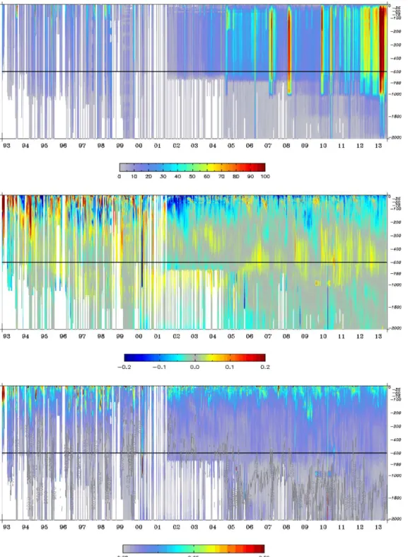
Finally, we present data assimilation diagnostics for tem-perature and salinity profile functions of the depth (Figs. 5 and 6). Diagnostics on the amount of assimilated data show that before the Argo era, i.e., before about 2005, there are few profiles deployed in the Mediterranean Sea, and most of them only reach 1000 m depth. Nonetheless, the mean inno-vation is close to zero on average between the surface and 2000 m depth for temperature and salinity. From 2005 to the end of the experiment, we note a positive anomaly (of ob-servation minus model) of about 0.2◦C and 0.03 psu around
Figure 3.Time series of weekly sea level anomaly (SLA; m) data assimilation statistics averaged over the whole Mediterranean basin: mean innovation (top) and rms of innovation (bottom). The colors stand for different satellites (please refer to Table 3).
Figure 4.Time series of weekly sea surface temperature (SST;◦C) data assimilation statistics from in situ (blue) and satellite SST AVHRR-AMSR (black), averaged over the whole Mediterranean basin : number of data (top), mean innovation (middle) and rms of innovation (bottom).
that started in 2003. Those positive anomalies at interme-diate depths suggest that the Levantine Intermeinterme-diate Water (LIW) in the model is too cold and too fresh compared to assimilated data in this layer. Conversely, the innovation in surface and deep layers shows a slight negative anomaly. On average, the rms of the innovation shows reasonable values compared to the mean innovation and the specified obser-vation errors but we note a clear seasonal variation, espe-cially for temperature profiles. During summer, the surface layers become more stratified. Due to the strong gradients, a small variation in the trajectory of the ocean model is then more likely to drift from observations and the rms naturally increases. Moreover, the cold bias in the surface associated with a warm bias in the subsurface illustrates that there is a lack of stratification in MEDRYS during summer.
Figure 5.Evolution of weekly temperature data assimilation statistics from in situ profiles, function of the depth averaged over the whole Mediterranean basin : number of observations (top), mean innovation (middle) and rms of the innovation (bottom).
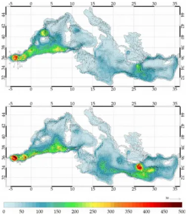
eddy in NM12-FREE experiment suggests that the model and its high-resolution atmospheric-forcing ALDERA are able to produce it but do not dissipate it afterward. This results in a large perturbation in the general circulation in west-ern Mediterranean in NM12-FREE. According to Fig. 7, the Liguro–Provençal current in NM12-FREE is deflected at the southern limit of the Gulf of Lions and a significant part of the AW is driven along the Spanish coast. This influences the circulation in the Algero–Provençal and the Alboran sub-basins. In MEDRYS, the assimilation process restores
real-istic surface circulation. The AW migrates into the western Mediterranean through the Strait of Gibraltar and reaches the Sicily channel through the Algerian current remaining close to the African coast.
in-Figure 6. Evolution of weekly salinity data assimilation statistics from in situ profiles, function of the depth averaged over the whole Mediterranean basin : number of observations (top), mean innovation (middle) and rms of the innovation (bottom).
jected by the assimilation process. We also notice that the Levantine sub-basin, and more specifically both the Ierape-tra and Pelops anticyclonic eddies, are more energetic sug-gesting that the mesoscale circulation components have been increased thanks to the assimilation of observational data.
3.2.3 Integrated temperature and salinity
Figure 7.Mean eddy kinetic energy (EKE; cm2s−2)at 40m depth over the period 1992–2013 for NM12-FREE (top) and MEDRYS (bottom). Arrows represent the mean currents (cm2s−1)over the
same period and at the same depth.
Llasses et al., 2015). Both products differ in the details of the mapping algorithm and the quality control applied to the observations. The difference between them can be viewed as a first estimate of the uncertainties linked to the obser-vational products, which cannot be neglected (Jordà and Gomis, 2013; Llasses et al., 2015). Basin integrals of the var-ious products are compared whatever real data are present or not. Monthly evolution over three different layers represent-ing surface (0–150 m), intermediate (150–600 m) and deep (600 m-bottom) waters are shown in Figs. 8 and 9.
The time series of the averaged temperature between the surface and 150 m depth in Fig. 8 point out the good rep-resentation of the seasonal cycle in both NM12-FREE and MEDRYS. The phase and the magnitude of the seasonal cy-cle are consistent with the EN3 and IMEDEA gridded prod-ucts. In terms of mean value, the two experiments are very close and present a positive bias compared to the gridded products. Indeed, in the 0–150 m layer, the difference be-tween the simulations and EN3 is about 0.15◦C and twice that compared to IMEDEA. This is also consistent with the assimilation statistics of in situ profiles shown in Sect. 3.2.1. In the upper layer, the averaged salinity in MEDRYS and NM12-FREE is comparable with that in EN3 and IMEDEA. However, between 1992 and 2013, MEDRYS shows a slight positive bias of about 0.02 psu, whereas NM12-FREE show
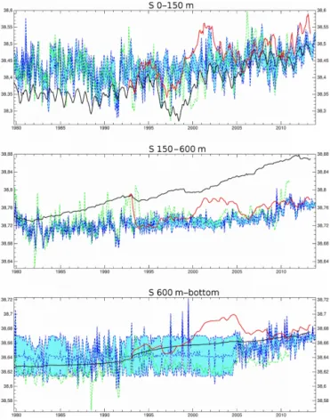
Figure 8.Evolution of the monthly integrated heat content (ex-pressed as mean temperature in◦C) over the Mediterranean basin for the layers 0–150 m (top), 150–600 m (middle) and 600 m-bottom (m-bottom) from MEDRYS (red line), NM12-FREE (black line), EN3 (dotted green line) and the IMEDEA (blue dotted line) hydrographic gridded products. The blue shaded area indicates the uncertainty ranges around the values of IMEDEA.
a slight negative bias of −0.03 psu compared to the
refer-ence products. Before 1993, the hindcast presents a clear negative bias of −0.07 psu. In 1993, the data assimilation corrects this surface salinity bias. The interannual variability of the atmospheric water fluxes (evaporation–precipitation– runoffs; not shown) present a less evaporative period fol-lowed by a stronger one in the late 90s and early 2000s. This leads to similar variability in the surface salt content in both MEDRYS and NM12-FREE. As there are few in situ data, especially for salinity, the stronger evaporation combined to a weak salinity constraint during the early 2000s leads to high surface salinization in MEDRYS.
Figure 9.Same as Fig. 8 but for integrated salt content (expressed as mean salinity in psu).
MEDRYS salinity in the early 2000s. Those too salty and too dense waters have been formed in the surface layers and have been advected toward the bottom layers. This bias is proba-bly explained by a bad adjustment of the volume correction term of the SLA model equivalent (Sect. 2.5). In Sect. 3.2.1, we noted that the mean SLA innovation (obs-model) was de-creasing, meaning that the simulated sea level tends to rise too quickly compared to the observations. In response to that, the system tends to compensate by densifying surface waters. As the assimilation system is more constrained on tempera-ture (due to better data coverage) it has a strong effect on salinity. The resulting bias is also detected in the bottom layer until 2005. Considering the small number of assimilated data below 600 m depth, the model is only slightly constrained be-yond this depth, especially before 2005. Thus, the reanalysis is quite close to the hindcast in terms of tendency and mean value for both temperature and salinity.
According to Fig. 8, it is difficult to establish whether both the hindcast and the reanalysis are able to represent a realistic temperature in the deepest layer. Actually, we cannot clearly distinguish any reference values as the two gridded products show different signals. However, the two experiments present a linear trend of warming of about 4×10⁻³◦C year−1
com-parable to EN3 for the 1993–2012 period IMEDEA presents
a lower warming of about 1.5×10⁻³◦C year−1. In the
deep-est layer, EN3 and IMEDEA show similar mean salinity (38.63 and 38.64 psu between 1979 and 2010, respectively) and a similar interannual variability. NM12-FREE presents a linear salinization over the whole period of the experiment in agreement with the gridded product (1.2×10⁻³psu year−1).
With a limited number of data to assimilate, MEDRYS shows an episode of high salinization from 1997 to 2004. Thanks to better data coverage after 2005, the reanalysis becomes more constrained and shows a more realistic average salinity, in accordance to our reference products.
Following Adani et al. (2011), the vertical distribution of the temperature and salinity anomalies is then presented in Figs. 10 and 11. Temperature and salinity anomalies have been computed with respect to the monthly cycle of the MEDATLAS-1979 climatology, from which the Octo-ber month has been taken to initialize NM12-FREE (see Sect. 2.2). These figures complete the vertical view given by Figs. 5 and 6, which were computed only at observation locations, and the integrated view given by Figs. 8 and 9. Moreover, this kind of diagnostics is presented in Adani et al. (2011) thus allowing for a qualitative comparison of two available reanalyses. For temperature, both NM12-FREE and MEDRYS show a similar behavior in the surface layer (above 100 m depth); we can thus attribute these anomalies to the model configuration (for instance issues with the ver-tical mixing) and to interannual variations, both simulations being forced by the same realistic atmospheric forcings in the surface. In the intermediate layer, NM12-FREE becomes slowly warmer and warmer, starting with a cold anomaly of about−0.1◦C in 1993 and ending with a warm anomaly of
about +0.2◦C in 2013, in the core of the LIW layer. For
MEDRYS, this core is too cold at about−0.2 to−0.1◦C,
this anomaly becoming smaller at the end of the period. In the bottom layer, NM12-FREE remains slightly colder than its initial state, around−0.1◦C, whereas MEDRYS shows a
slight warming during the 20 years, in agreement with Fig. 8. For salinity, again the anomalies above 100 m depth are similar in both simulations; the succession of positive and negative anomalies can be related to interannual variability. Nevertheless, the surface layer is more salty in MEDRYS than in NM12-FREE, especially during the last years. In the intermediate layer, around the core of the LIW layer, NM12-FREE becomes saltier and saltier during the 20 years, from
anoma-Figure 10.NM12-FREE basin mean temperature (◦C, above) and salinity (psu, below) anomalies with respect to MedAtlas-1979.
Figure 11.MEDRYS basin mean temperature (◦C, above) and salinity (psu, below) anomalies with respect to MedAtlas-1979.
lies up to+0.1 psu. Moreover, the positive anomalies in the surface layer in MEDRYS around year 2000 seems to propa-gate downwards (as seen in Fig. 9), leading to the end of the negative anomaly in the intermediate layer between 2001 and
2005 and to a stronger positive anomaly in the bottom layer between 2002 and 2006.
similar patterns in both reanalyses: high variability in the surface layer, a slightly too cold intermediate layer, and a deep layer becoming warmer and saltier during the simu-lated period, the amplitude of the anomalies being smaller in MEDRYS. As these reanalyses are performed with different numerical modeling choices, different atmospheric forcing and different assimilation schemes, these common features could be related to realistic physical processes, which could be interesting to assess in a common dedicated work. 3.2.4 Temperature and salinity vertical profiles
The model equivalent at the time and spatial location of the observations has been computed from daily aver-aged outputs. Mean and rms differences over the whole Mediterranean basin were computed for three layers (0–150, 150–600, 600–4000 m) for temperature and salinity profiles (CLASS4) and are presented in Figs. 12 and 13. In or-der to evaluate the improvement with respect to a constant state, we applied the same process with the profiles from MEDATLAS-1998. The MEDATLAS-1998 temperature and salinity fields are the initial states of short simulations used for process studies such as in Beuvier at al. (2012a). Those fields have been obtained applying a low-pass filter with a time window of 3 years on the MEDATLAS data covering the 1997-1999 period. The choice of centering the climatol-ogy on the late 90s corresponds to a compromise between a recent year (before 2002, the last field in MEDATLAS) and a sufficient data coverage in both temperature and salin-ity, knowing that the uncertainty associated with the ME-DATLAS fields increases after 2000. Only daily data sets, checked through objective quality control, have been assim-ilated in MEDRYS. Large differences may appear locally in the CLASS4 scores with spurious observations. CLASS4 results complement here the statistics made against 1-week forecasts in Sect. 3.2.1.
We first assess the mean and rms temperature differences between the analysis and the observations in Fig. 12. Con-cerning the layer-averaged mean differences, results are not fully consistent with comparisons made with integrated con-tent in Sect. 3.2.3. Indeed, those statistics show that, on aver-age, MEDRYS is very close to the observations (at the loca-tion of the observaloca-tions). We only note a significant negative bias of 0.03◦C in the layer 150/600 m on average over the
pe-riod 1993–2012. The mean temperature difference in the two first layers of the reanalysis reproduces the interannual vari-ability present in the observations. As MEDATLAS-1998 is a climatology, the magnitude of the oceanic interannual vari-ability is then represented by the blue curve. We also point out that, on average, no particular temperature bias occurred in the deepest layer in MEDRYS. This highlights that the sys-tem is well constrained and efficiently responds to the assimi-lation of in situ profiles. On average MEDRYS remains close to temperature measurements, and this also confirms that the reference products shown in the Sect. 3.2.3 are subject to
un-certainties, especially in the deepest layers where the esti-mated mean temperature may vary widely from one prod-uct to another. In terms of mean salinity (Fig. 13), MEDRYS is also close to the observations in the deepest layers but, as expected, presents a slight positive bias of about 0.02 psu between the surface and 150 m depth. When we compared the integrated salinity of the reanalysis with other gridded products, we noted a spurious salinization in MEDRYS in the early 2000s that propagated toward deeper layers. On av-erage, the CLASS4 mean difference in salinity is only about 0.1 psu between the surface and 150 m depth and is not no-ticeable below. Assuming that the major part of the salinity observations are used in both MEDRYS and the reference gridded products, this suggests that the signal of the deeper salinization is not in the observations but is a consequence of the propagation of the simulated surface anomaly through the ocean model. However, as the uncertainties in the salin-ity products are large (Llasses et al., 2015), it cannot be dis-carded that the observational products missed that change.
The rms of the difference is quite good both in temper-ature and salinity considering the variability in the differ-ent layers. However, we note that the rms of the difference in salinity increases in the waters deeper than 600 m, mean-ing that, despite a realistic estimation of the mean value, the spatial variability is not robust. This can be explained by the lack of salinity measurements and the poor data cover-age in Mediterranean Sea under 1000 m depth, especially be-fore 2005. On average, MEDRYS presents a lower rms of the difference of temperature and salinity than MEDATLAS-1998. It is not surprising considering that MEDATLAS-1998 is composed of climatological monthly fields and does not represent the variability of the Mediterranean Sea along the whole period of 21 years. In the first 150 m, the rms of the difference in MEDRYS increases with the summertime strat-ification.
3.2.5 High-frequency variability: comparison at LION buoy
Figure 12.Temperature (◦C) mean (upper row) and rms (bottom row) differences analysis minus observation (black), and MEDATLAS-1998 minus observation (blue). For these diagnostics, all availableT /Sobservations from the CORIOLIS database and MEDRYS daily average analysis, collocated (temporally and spatially) with observations, are used. The number of observations is shown with gray bars. Averages are performed in the 0–150m (left), 150–600 m (middle) and 600–4000 m (right) layers in the whole Mediterranean basin.
For both SST and SSS comparisons, MEDRYS is slightly closer to the independent observations than the hindcast, in terms of mean values and variability. Indeed, the mean sur-face water of MEDRYS shows a positive bias of 0.07◦C and 0.03 psu while NM12-FREE shows negative biases which are larger in magnitude (0.13◦C and 0.06 psu). The major part
of the mean bias in SSS between MEDRYS and the obser-vations can be explained by the large difference during Jan-uary (+0.1 psu on average) because the mean bias afterward is very weak (less than 0.01 psu). Indeed, we notice a strong jump in the observed SSS, which on 30 January (+0.04 psu)
corresponds to a salinity sensor repair (M. N. Bouin, per-sonal communication, 2015). The water-pump was defective and affected the conductivity measurement. Assuming that a constant negative bias of 0,04 psu contaminated the obser-vation during January, MEDRYS finally presents very good results in SSS during SOP2 at the LION buoy.
Figure 13.Same as Fig. 12 but for salinity (psu).
This is not surprising since the variability at the surface is controlled by fluxes (identical for both experiments) dur-ing the mixed phase of the convection. We especially note the good representation in phase and amplitude of the di-urnal variations of SST. This is especially obvious around the 20 February and during many days in March during a temporary re-stratification period, when the diurnal cycle of ALDERA heat fluxes have a higher daily amplitude (begin-ning of spring season).
3.2.6 Transport through the Strait of Gibraltar
We present here water, heat and salt transport through the Strait of Gibraltar at 5.5◦W in Fig. 15. Heat and salt fluxes
are computed from temperature (T) and salinity (S) using Eqs. (1) and (2). Ux represents the zonal component of the current at 5.5◦W, ρ
0 is the reference sea water density
(1020 Kg m−3),S
med andVmedare respectively the surface
and the volume of the simulated Mediterranean Sea andNsec
is the number of seconds in a year. Characteristics of the in-flow (surface layers) and the outin-flow (deep layers) and the difference between the two (net flow) are presented. The in-terface between inflow and outflow has been determined us-ing the horizontal velocity through the strait at daily time-scale.
HeatFluxgib= ρ0Cp
Smed Z Z
Figure 14.Evolution of the hourly sea surface temperature (SST; top) and sea surface salinity (SSS; bottom) at the LION buoy loca-tion (red dot on the map) between 1 January and 31 March 2013. The observation is shown with the green lines, NM12-FREE with the black lines and MEDRYS with the red lines.
SaltFluxgib= Nsec Vmed
Z Z
S (y, z) Ux(y, z)dydz (2) Although the characteristics of the ocean are the same in the buffer zone in the two experiments, the amplitude of both inflow and outflow has been improved thanks to data assimilation in MEDRYS (Fig. 15). Despite the realistic value of the net flow through the Strait of Gibraltar, out-flow and inout-flow are underestimated in NM12-FREE in com-parison with recent results published (Soto-Navarro et al., 2010, 2014). According to those studies, the acceptable range for inflow and outflow at Gibraltar Strait are respec-tively [+0.76; +0.86] Sv and [−0.84; −0.72] Sv. The rea-son of having a more accurate exchange at Gibraltar in MEDRYS is that the density difference between the in-flowing and outin-flowing waters is larger (−2.34 kg m−3 in
MEDRYS and−2.30 kg m−3in NM12-FREE). In terms of
net heat transport, the reanalysis and the hindcast (respec-tively 6.6±0.4 W m−2and 5.5±0.4 W m−2) are consistent
with MacDonald et al. (1994). We also compare the proper-ties of the inflow in MEDRYS and NM12-FREE with results from Soto-Navarro et al. (2014) at the sill of Espartel. They used, inter alia, the experiment NM12-ARPERA. This sim-ulation shows similar results with an interface around 150 m depth. At this particular depth, we also report similar results with AW at 15.4◦C and 36.7 psu in MEDRYS and at 15.5◦C and 36,5 psu in NM12-FREE.
The net salt transport through the Strait of Gibraltar at 5.5◦W is 1.8±2.8×10⁻³psu year−1 in MEDRYS and
3.0±2.6×10⁻³psu year−1 in NM12-FREE (Fig. 14).
As-Figure 15.Average flow, heat and salt transport of the inflow and the outflow through the Strait of Gibraltar at 5.5◦W between 1992 and 2013 for NM12-FREE and MEDRYS. The uncertainty corre-sponds to the annual standard deviation. For heat and salt transport, the associated mean temperature and salinity in the layer are spec-ified. The green color represents values consistent with literature or/and reference products and the red color those that are not con-sistent.
suming that the Mediterranean volume is constant, the evo-lution of Mediterranean salinity is directly linked to the net transport of salt through the Strait of Gibraltar. The trend in salinity (1sref) of the reference hydrographic gridded prod-ucts (EN3 and IMEDEA) over the whole basin serves as a way to estimate a reference net salt transport entering at Gibraltar (SaltFluxgibfrom Eq. 2), using SaltFluxgib=1sref.
From the hydrographic products, we estimate a reference net salt intake at approximately 1.7×10⁻³psu year−1between
1993 and 2012. In MEDRYS, the averaged net salt transport through the Strait of Gibraltar is very close to this reference value but this is not representative of the evolution of the salinity over the whole basin because of the addition of salin-ity increments coming from the assimilation scheme. Indeed, NM12-FREE and MEDRYS have a similar trend in salinity in spite of a different net salt transport at Gibraltar.
4 Discussion and conclusion
repro-duce a diurnal cycle and thus SST, and to simulate the im-pact of local winds on coastal oceanic areas. As we payed special attention to reducing sources of inhomogeneity in the atmospheric-forcing ALDERA data set along the whole 1979–2013, this suggests one should trust the consistency of the interannual variability of processes known to be driven by air–sea interactions (mixed layer variability, surface cir-culation variability, etc.) in MEDRYS.
The validation process has highlighted the good results of the reanalysis in terms of mean circulation and integrated heat and salt contents. The data assimilation has a positive impact, especially in the western basin, where it restores a correct circulation of the Liguro–Provençal current and of the Algerian current. The assimilation process leads to stronger mesoscale variability in the Ionian and Levantine sub-basin, especially at the location of Ierapetra and Pelops eddies. Looking at in situ profiles, the reanalysis shows realistic wa-ter masses at inwa-termediate depths, unlike in the hindcast. In this layer, the simulation without assimilation NM12-FREE drifts from the observations and shows a strong positive trend in both temperature and salinity. Transports through the Strait of Gibraltar have also been improved in the reanalysis. De-spite the same forcing in the Atlantic buffer zone, both inflow and outflow in MEDRYS have been increased compared to NM12-FREE and are now comparable to historical values. The net heat and salt budgets through the strait are also con-sistent with independent products. The improvement of the Atlantic/Mediterranean fluxes at Gibraltar ensures a better budget in the Mediterranean Sea.
We showed that surface waters in MEDRYS were on aver-age too salty (about 0.02 psu). This problem probably comes from the adjustment of the volume correction during the computation of the SLA model equivalent. We also point out that it had inconsistencies between ORAS4 interannual fields in the buffer zone and the assimilated data. To correct for those inconsistencies, it will be necessary to apply a cor-rection to the ORAS4 SSH fields in order to better represent the seasonal variations of sea level in the Mediterranean. In further version of MEDRYS, we simply propose to correct the seasonal cycle and the trends of sea level anomalies in ORAS4 in order to match with altimetry observations in the buffer zone. According to additional works (not shown in this study), we realized that SLA innovations were strongly correlated with the mean wind patterns (Mistral-Tramontane, Aegean winds), suggesting that the hydraulic constraint com-ponent is not negligible in the Mediterranean Sea. Knowing that, the configuration of SAM2 should be adjusted in order to take into account the wind component in SSH. Moreover, as the effect of the wind at high frequency has been filtered from the SSALTO/DUACS database, it would be also neces-sary to filter it in the model.
Acknowledgements. We acknowledge the two anonymous
re-viewers for their comments and suggestions, which helped to improve this article. This work is a contribution to the HyMeX program (HYdrological cycle in The Mediterranean EXperiment) through INSU-MISTRALS support and the Med-CORDEX program (COordinated Regional climate Downscaling EXperiment – Mediterranean region, www.medcordex.eu). This research has received funding from the French National Research Agency (ANR) project REMEMBER (contract ANR-12-SENV-001).
Edited by: N. Pinardi
References
Adani, M., Dobricic, S., and Pinardi, N.: Quality assessment of a 1985–2007 Mediterranean Sea reanalysis, J. Atmos. Ocean. Tech., 28, 569–589, doi:10.1175/2010JTECHO798.1, 2011. Auger, P. A., Ulses, C., Estournel, C., Stemman, L., Somot, S., and
Diaz, F.: Interannual control of plankton ecosystem in a deep convection area as inferred from a 30-year 3D modeling study: winter mixing and prey/predator in the NW Mediterranean, Prog. Oceanogr., 12–27, doi:10.1016/j.pocean.2014.04.004, 2014. Ayoub, N., Le Traon, P.-Y., and De Mey, P.: A description of the
Mediterranean surface variable circulation from combined ers-1 and topex/poseidon altimetric data, J. Marine Syst., ers-18, 3–40, doi:10.1016/S0924-7963(98)80004-3, 1998.
Balmaseda, M. A., Trenberth, K. E., and Källén, E.: Distinctive cli-mate signals in reanalysis of global ocean heat content, Geophys. Res. Lett., 40, 1754–1759, doi:10.1002/grl.50382, 2013. Barnier, B., Siefridt, L., and Marchesiello, P.: Thermal forcing for a
global ocean circulation model using a three-year climatology of ECMWF analyses. J. Marine Syst., 6, 363–380, 1995.
Béranger, K., Mortier, L., and Crépon, M.: Seasonal variability of water transport through the Straits of Gibraltar, Sicily and Cor-sica, derived from a high-resolution model of the Mediterranean circulation, Prog. Oceanogr., 66, 341–364, 2005.
Béranger, K., Drillet, Y., Houssais, M.-N., Testor, P., Bourdallé-Badie, R., Alhammoud, B., Bozec, A., Mortier, L., Bouruet-Aubertot, P., and Crépon, M.: Impact of the spatial distri-bution of the atmospheric forcing on water mass formation in the Mediterranean Sea, J. Geophys. Res., 115, C12041, doi:10.1029/2009JC005648, 2010.
Beuvier, J., Sevault, F., Herrmann, M., Kontoyiannis, H., Lud-wig, W., Rixen, M., Stanev, E., Béranger, K., and Somot, S.: Modeling the Mediterranean Sea interannual variability during 1961–2000: focus on the Eastern Mediterranean Transient, J. Geophys. Res., 115, C08017, doi:10.1029/2009JC005950, 2010. Beuvier, J., Béranger K., Lebeaupin-Brossier, C., Somot, S., Se-vault, F., Drillet, Y., Bourdalle-Badie, R., Ferry, N., and Lyard, F.: Spreading of the Western Mediterranean Deep Water after winter 2005: time scales and deep cyclone transport, J. Geophys. Res.-Oceans, 117, C07022, doi:10.1029/2011JC007679, 2012a. Beuvier, J., Lebeaupin-Brossier, C., Béranger, K., Arsouze, T.,