www.atmos-chem-phys.net/12/5207/2012/ doi:10.5194/acp-12-5207-2012
© Author(s) 2012. CC Attribution 3.0 License.
Chemistry
and Physics
Technical Note: A trace gas climatology derived from the
Atmospheric Chemistry Experiment Fourier Transform
Spectrometer (ACE-FTS) data set
A. Jones1, K. A. Walker1,2, J. J. Jin3, J. R. Taylor4,5, C. D. Boone2, P. F. Bernath6,7, S. Brohede8, G. L. Manney3,9, S. McLeod2, R. Hughes2, and W. H. Daffer3
1Department of Physics, University of Toronto, Toronto, Canada
2Department of Chemistry, University of Waterloo, Waterloo, Ontario, Canada 3Jet Propulsion Laboratory, California Institute of Technology, Pasadena, CA, USA 4National Center for Atmospheric Research, Boulder, CO, USA
5National Ecological Observatory Network, Boulder, CO, USA
6Department of Chemistry and Biochemistry, Old Dominion University, Norfolk, Virginia, USA 7Department of Chemistry, University of York, Heslington, York, UK
8Department of Radio and Space Science, Chalmers University of Technology, Gothenburg, Sweden 9New Mexico Institute of Mining and Technology, Socorro, New Mexico, USA
Correspondence to:K. A. Walker ([email protected])
Received: 20 July 2011 – Published in Atmos. Chem. Phys. Discuss.: 7 November 2011 Revised: 25 April 2012 – Accepted: 18 May 2012 – Published: 14 June 2012
Abstract.The Atmospheric Chemistry Experiment-Fourier Transform Spectrometer (ACE-FTS) aboard the Canadian satellite SCISAT (launched in August 2003) was designed to investigate the composition of the upper troposphere, strato-sphere, and mesosphere. ACE-FTS utilizes solar occultation to measure temperature and pressure as well as vertical pro-files of over thirty chemical species including O3, H2O, CH4,
N2O, CO, NO, NO2, N2O5, HNO3, HCl, ClONO2, CCl3F,
CCl2F2, and HF. Global coverage for each species is obtained
approximately over a three month period and measurements are made with a vertical resolution of typically 3–4 km. A quality-controlled climatology has been created for each of these 14 baseline species, where individual profiles are av-eraged over the period of February 2004 to February 2009. Measurements used are from the ACE-FTS version 2.2 data set including updates for O3 and N2O5. The climatological
fields are provided on a monthly and three-monthly basis (DJF, MAM, JJA, SON) at 5 degree latitude and equivalent latitude spacing and on 28 pressure surfaces (26 of which are defined by the Stratospheric Processes And their Role in Climate (SPARC) Chemistry-Climate Model Validation Activity). The ACE-FTS climatological data set is available through the ACE website.
1 Introduction
Coupled Chemistry-Climate models (CCMs) and General Circulation Models (GCMs) are widely used by the scientific community to improve our understanding of the atmosphere. In the middle atmosphere, such models play a key role in pre-dictions of stratospheric ozone loss, which has been a main concern for more than two decades. In addition, atmospheric climate models are useful in investigating atmospheric re-sponses to fluctuations in solar intensity, to changes in key greenhouse gases (e.g. carbon dioxide), to volcanic activity, and to changes in other radiative forcing parameters, which collectively are significant processes in controling climate change.
This may be done by comparing models to each other, but also needs to be accompanied by comparing model simula-tions to well-characterized trace gas observasimula-tions, which are often provided in the form of a climatological average. Fur-thermore, climatological data can provide information about what assumptions should be made concerning initial condi-tions and input parameterizacondi-tions and can be used to con-strain various model parameters as necessary. In addition, cli-matological data can be used for analysis of tracer transport and of inter-annual variability, leading to a better understand-ing of the dynamical and chemical processes involved (e.g. Randel et al., 1998).
Observational climatology data is widely used and is a comprehensive way of representing data over specific pe-riods of time. There are various long-term climatological products available based on the measurements of the mid-dle atmosphere that have been reported over the last 14 yr. The earliest ozone climatology was compiled by Fortuin and Kelder (1998) using an amalgamation of data pro-vided by ozonesondes and the Solar Back-scatter Ultra-Violet (SBUV) instrument for the period of 1980–1991. Ran-del et al. (1998) produced CH4and H2O climatologies
us-ing data collected durus-ing 1991–1997 by the Upper Atmo-spheric Research Satellite (UARS) Halogen Occultation Ex-periment (HALOE) instrument (Russell et al., 1993), while Beaver and Russell produced HCl and HF climatologies for the first 4.5 years of the HALOE mission (1998). A water vapour climatology was produced by Chiou et al. (1997) us-ing data from the Stratospheric Aerosol and Gas Experiment SAGE II instrument. A comprehensive HALOE climatol-ogy product was compiled by Grooß and Russell (2005) for O3, CH4, H2O, HF, HCl, and NOx using data from 1991–
2002. McPeters et al. (2007) used a similar technique to Fortuin and Kelder to compile an ozone climatology for 1988–2002 using data from ozonesondes and the SAGE II and UARS Microwave Limb Sounder (UARS-MLS) satellite instruments. The UARS reference atmosphere project pro-vides climatologies for some key atmospheric species utiliz-ing measurements from various UARS instruments durutiliz-ing their lifetime of 1991–2005 (http://umpgal.gsfc.nasa.gov/). Hoffmann et al. (2008) produced a CCl3F (CFC-11)
up-per troposphere/lower stratosphere climatology for 2002– 2004 using data from the Michelson Interferometer for Pas-sive Atmospheric Sounding (MIPAS) instrument on Envisat. The Odin Sub-Millimetre Radiometer (Odin-SMR) HNO3
and Odin Optical Spectrograph and InfraRed Imager System (Odin-OSIRIS) NO2 data were combined with a chemical
box model to produce an NOy climatology for 2002–2006
(Brohede et al., 2008). A separate Odin SMR HNO3
clima-tology has also been produced for the period 2001–2009 (Ur-ban et al., 2009). Recently, Jones et al. (2011) created an NOy
climatology using 2004–2009 measurements from the At-mospheric Chemistry Experiment Fourier Transform Spec-trometer (ACE-FTS) following the methodology described herein.
Here, we present a climatology that utilizes data from ACE-FTS between 2004 and 2009. This data set is intended to complement the existing climatologies from HALOE and other instruments (as described above) by providing infor-mation for a larger number of species (fourteen in total) in a consistent data set. This will provide a source of data for model intercomparison studies and other atmospheric research projects. For example, the range of chlorine- and nitrogen-containing trace gases measured by ACE-FTS can provide information about how these species are partitioned within families. In the following section, we give a summary of the ACE mission as well as introduce the main species for which the climatologies are produced, including a summary of the relevant validation results for each species. Section 3 describes the methodology used to produce the climatolo-gies. Finally, Sect. 4 illustrates selected results for the clima-tological products.
2 Description of ACE-FTS and its data products
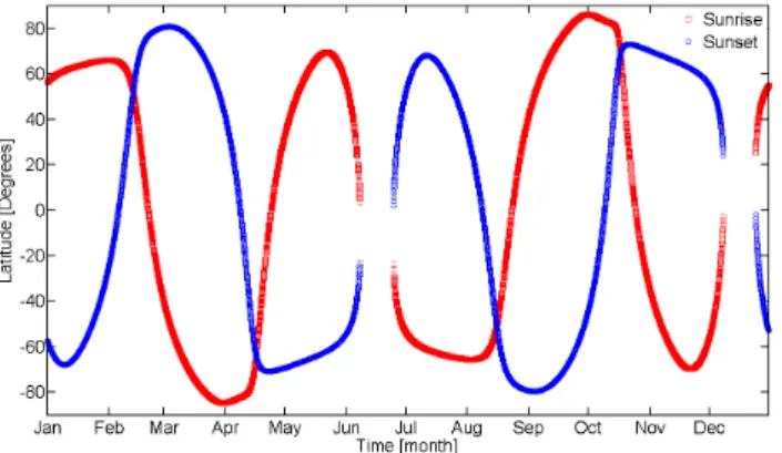
The ACE mission is on-board the SCISAT satellite which was put into orbit on 12 August 2003. SCISAT is a Canadian-led satellite mission, which carries two main instruments to study atmospheric composition: the ACE Fourier Trans-form Spectrometer (ACE-FTS) (Bernath et al., 2005), and the Measurement of Aerosol Extinction in the Stratosphere and Troposphere Retrieved by Occultation (ACE-MAESTRO) (McElroy et al., 2007). Measurements taken by both of these instruments utilize solar occultation geometry, making up to 15 sunset and 15 sunrise measurements per day. In addi-tion to these instruments, there is a two channel visible/near-infrared imager (ACE-IMAGER) that yields extinction pro-files at 0.525 µm and 1.02 µm (Gilbert et al., 2007). The SCISAT satellite is in a circular orbit at 650 km altitude with a 74 degree inclination angle to the equator. It has an annu-ally repeating pattern of measurement latitudes (as shown in Fig. 1). During a 12 month period, the ACE orbit allows global measurements to be made from 85◦S to 85◦N with all latitudes covered during each three-month season.
The ACE-FTS measurements provide vertical profiles of more than 30 atmospheric species, temperature, and pressure from spectra measured between 750 and 4400 cm−1(2.2 to 13 µm) at a resolution of 0.02 cm−1(Bernath et al., 2005). Information about the processing of the measured spectra is provided by Boone et al. (2005). Briefly, the retrieval process uses a two step sequence. Firstly, both atmospheric pressure and temperature are retrieved using microwindows contain-ing CO2 spectral lines. Then the pressure and temperature
Fig. 1.Latitude versus time of ACE-FTS observations for one year. The SCISAT satellite maintains an annually repeating pattern of measurement latitudes.
grid (tangent height) and are also interpolated onto a 1-km grid using a piecewise quadratic method. For this project, the profiles on the measurement grid have been used.
The 14 baseline atmospheric species measured by ACE-FTS are O3, H2O, HCl, CCl3F, CCl2F2, CH4, HF, N2O,
CO, NO, NO2, HNO3, ClONO2, and N2O5. We use
ver-sion 2.2 of ACE-FTS retrievals (including updates for O3
and N2O5), all of which have been validated. At present,
no error budget estimates have been made for this data set. The following are descriptions of each species with a short summary of the validation results, highlighting the biases between ACE-FTS and other atmospheric pro-file data sets. For a more comprehensive description for each species, the reader is directed to the relevant arti-cle. The referenced articles are part of the ACE valida-tion results special issue (http://www.atmos-chem-phys.net/ special issue114.html). For each species, the title of the sub-section contains the relevant validation reference and the typ-ical retrieval altitude range.
2.1 O3– Dupuy et al. (2009) (5–95 km)
This work uses the version 2.2 ozone update. For this ver-sion, there is a small positive bias, between ACE-FTS and correlative satellite and ozonesonde measurements, typi-cally of +1 to +8 % in the stratosphere (16–44 km). Above 45 km, ACE-FTS ozone values are significantly larger than the comparison instruments by up to +40 % (+20 % on av-erage). These comparisons were made with solar occulta-tion instruments, such as HALOE (v19), SAGE II (v6.2), SAGE III (v3.0), and POAM III (v4.0), and other satel-lite measurements, including GOMOS (IPF v5.0), SCIA-MACHY (IUP v1.63), Aura-MLS (v2.2), and MIPAS (ESA v4.62, ML2PP/5, V3O O3 7). No significant differences were found in the biases for sunrise and sunset occultations.
2.2 H2O – Carleer et al. (2008) (5–89 km)
Coincident satellite measurements from SAGE II (v6.2), HALOE (v19), MIPAS (v13 IMK-IAA), and Odin SMR (v2.1) have been compared with ACE-FTS H2O. In these
comparisons, ACE-FTS has a small positive bias of 3–10 % between 15 and 90 km. In comparisons with POAM III (v4.0), there is a negative bias for ACE-FTS between 15 and 39 km that is consistent with earlier POAM III comparisons.
2.3 HCl – Mahieu et al. (2008) (8–57 km)
Comparisons of coincident measurements from ACE-FTS and Aura MLS (v2.2) show agreement better than 5 % be-tween 100 and 0.1 hPa (∼16–60 km). Comparisons to the HALOE instrument (v19) show that there is a bias between coincident measurements of +10–15 % in the stratosphere (approximately 20–50 km). A similar bias is seen in com-parisons between Aura MLS and HALOE (Froidevaux et al., 2008). Furthermore, a comparison of an ACE-FTS zonal mean profile and profiles from the balloon-borne MkIV dur-ing the autumn of 2003, 2004 and 2005 around 35◦N yields agreement of better than±7 % up to 20 km.
2.4 CCl3F (CFC-11) – Mahieu et al. (2008) (5–22 km)
There were limited CFC satellite data available for the Mahieu et al. (2008) validation analysis. Thus comparisons were made with balloon-borne measurements from FIRS-2 and MkIV. The differences between individual ACE-FTS and FIRS-2 profiles are typically−10 % from 12 to 16 km, where the ACE-FTS VMRs are slightly smaller than FIRS-2. An ACE-FTS zonal mean profile is systematically smaller than coincident MkIV profiles by typically−10 % above 12 km and up to−20 % below 12 km.
2.5 CCl2F2(CFC-12) – Mahieu et al. (2008) (6–28 km)
As was done for CCl3F, ACE-FTS CCl2F2 profiles were
compared to FIRS-2 and MkIV balloon profiles. ACE-FTS measurements were averaged to create a zonal mean profile to compare with the MkIV 2004 and 2005 profiles. These comparisons show a maximum bias of −10 % between 10 and 28 km. The comparison of individual profiles from ACE-FTS and FIRS-2 show large systematic biases of±50 % be-tween 12 and 21 km. However, bebe-tween 17 and 24 km, these differences are within the uncertainty of the FIRS-2 measure-ment.
2.6 CH4– De Mazi`ere et al. (2008) (5–62 km)
to 60 km. A comparison with a January 2006 high-latitude profile from the balloon-borne SPIRALE instrument showed that there is a small bias between ACE-FTS and SPIRALE that is smaller than±10 % between 15 and 24 km.
2.7 HF – Mahieu et al. (2008) (10–50 km)
As was found for HCl, coincident ACE-FTS and HALOE (v19) measurements show an ACE-FTS bias of typically +5– 20 % between 15 and 49 km. Additionally, a comparison of a zonal average ACE-FTS profile (as no direct comparisons were found) to the 2004 and 2005 MkIV balloon profiles agree better than±10 % above 19 km.
2.8 N2O – Strong et al. (2008) (5–60 km)
ACE-FTS N2O profiles were compared with measurements
from Odin SMR (v2.1), Aura MLS (v2.2) and MIPAS (ESA, v4.62 and IMK-IAA, v3.0). The relative differences for these data sets are within ±15 % between 6 and 30 km, except for MIPAS near 30 km where the differences are as large as −22.5 %. Between 30 and 60 km, the absolute differences for the satellite comparisons typically range from−2 to +1 ppbv. Relative differences are not given because the N2O VMR is
quite small over this altitude range.
2.9 CO – Clerbaux et al. (2008) (5–105 km)
The agreement with correlative satellite limb measurements, including MIPAS (version 9.0) and Odin SMR (v2.1), is typ-ically better than 30 % from 20 to 100 km. Larger differences were found in comparisons with Aura MLS because there was greater noise in the MLS profiles than in the ACE-FTS ones. Between 6 and 14 km, agreement of±2 % or better was found in comparisons with nadir measurements by MOPITT and TES. For these comparisons, the ACE-FTS profiles were smoothed using the averaging kernels of the lower resolution instruments.
2.10 NO – Kerzenmacher et al. (2008) (12–105 km)
Comparisons made to the HALOE (v19) data set show rel-ative differences that are less than±20 % below 60 km and typically better than ±8 % between 22 km and 60 km. Be-tween 60 and 90 km, ACE-FTS is biased low compared to HALOE (∼80 %), although the one sigma uncertainty in the systematic biases is often zero, implying that statistical dif-ferences are not significant. ACE-FTS also shows a typical +10 % bias compared to HALOE from to 93 km to 105 km.
2.11 NO2– Kerzenmacher et al. (2008) (12–105 km)
The relative differences from comparisons of ACE-FTS to SAGE II (v6.2), HALOE (v19), and MIPAS (IMK-IAA, v3.0) are typically better than±20 % throughout the strato-sphere (∼20–50 km), with slightly better than 10 %
system-atic bias resulting from ACE-FTS coincidences with SCIA-MACHY (v2.0, occultation and nadir), GOMOS (IPF 5.0), and SAGE III (v3.0). Comparisons with Odin OSIRIS (v3.0) yield a relative difference of typically less than 6 % between 14 and 24 km and 13 % above 25 km. ACE-FTS exhibits a consistent low bias compared to MIPAS (ESA, v4.62) of −8 % and−45 % in the lower and upper stratosphere respec-tively. This study used a chemical box model (McLinden et al., 2000; McLinden 2006) for comparisons to GOMOS and OSIRIS so as to account for the strong diurnal effect of NO2.
Here, scale factors were calculated to re-scale GOMOS and OSIRIS NO2measurements to the local solar times (LSTs)
of the ACE-FTS coincidences.
2.12 HNO3– Wolff et al. (2008) (5–37 km)
The agreement between coincident measurements from Odin SMR (v2.0), MIPAS (ESA v4.62, IMK-IAA v8.0), and MLS (v2.2) is typically better than 20 % (and often within 10 %) for the overlapping altitude ranges of each instrument.
2.13 ClONO2– Wolff et al. (2008) (5–37 km)
Comparisons with coincident MIPAS (IMK-IAA v11.0) data show agreement to better than ±1 % from 16–27 km and within +14 % from 27–34 km. As ClONO2has some diurnal
variation, these comparisons required the use of a chemistry transport model (Kouker et al., 1999) to transform the MI-PAS observations to the time and location of the ACE-FTS occultations.
2.14 N2O5– Wolff et al. (2008) (5–37 km)
Similar to the ozone validation, this work uses the ACE-FTS v2.2 N2O5update. Below 27 km, relative differences
be-tween ACE-FTS and MIPAS (IMK-IAA v9.0) are typically better than−10 % and−27 % during daytime and nighttime, respectively. To account for the strong N2O5diurnal
varia-tion, the same chemistry transport model was employed as was used for the ClONO2study.
3 Methodology
In order to discuss the production of a climatology, it is first useful to provide a definition. Simply put, a climatology is the average state of an atmospheric parameter over a given time period with respect to altitude and geolocation coordi-nates. Typically, a climatology is provided as a function of al-titude (or pressure), laal-titude (or equivalent laal-titude) and time (month or season).
3.1 ACE climatology grid description
90, 80, 70, 50, 30, 20, 15, 10, 7, 5, 3, 2, 1.5, 1, 0.5, 0.3, 0.2, 0.1 hPa (SPARC CCMVal, 2010). The other two pres-sure levels are added in the upper stratosphere and lower mesosphere, namely, 0.7 and 0.15 hPa. These pressure lev-els are the centres of each bin. The limits of each bin are calculated to be equidistant from the adjacent centres in log pressure. The horizontal coordinate is divided into 5 degree intervals from 90◦S to 90◦N (e.g. the 90◦S to 85◦S interval is labeled as 87.5◦S).
3.2 Filling the grid
The ACE-FTS climatologies are made for O3, H2O, CH4,
N2O, CO, NO, NO2, N2O5, HNO3, HCl, ClONO2, CCl3F,
CCl2F2, and HF on a monthly and three-month combined
basis using the set of more than 19 000 occultation measure-ments obtained between late February 2004 and late Febru-ary 2009. The yearly latitude coverage of the ACE measure-ments is shown in Fig. 1. ACE obtains global latitude cover-age over a period of approximately three months. This means that for any given month there will be gaps in the climatol-ogy as certain latitudes will not be measured due to the na-ture of the SCISAT orbit. In addition to making climatolo-gies arranged by latitude, we also compile climatoloclimatolo-gies on an equivalent latitude grid. Equivalent latitude is a vortex-centred coordinate system based on the area enclosed by potential vorticity contours (Butchart and Remsberg, 1986). This is a useful parameter since, in addition to insuring that data averaged together are from similar air masses, it also allows for a broader coverage to be attained due to the varia-tions in potential vorticity at a given latitude, thus helping to fill some of the gaps that would occur in the latitude clima-tology fields. For each ACE-FTS profile, equivalent latitude, as a function of altitude, is available as part of the suite of “derived meteorological products” (DMPs) as described in Manney et al. (2007). To calculate these DMPs, the GEOS-5 meteorological fields (Rienecker et al., 2008) are interpo-lated to the location and time of the ACE-FTS measurement (Manney et al., 2007).
Some of the species measured by ACE-FTS have diurnal variations (such as NO, NO2, HNO3, ClONO2, and N2O5).
In order to account for this, we consider the local solar time (LST) of the measurements, such that separate climatologies are produced for AM (before local solar noon) and PM (after local solar noon) in addition to a climatology based on all occultations (AM + PM). LST is calculated by considering the universal time (UTC) and the longitude (φ, defined as −180◦to +180◦) of each occultation at the ACE-FTS 30 km reference tangent point as was done in Nassar et al. (2006),
LST=UTC+(24/360)φ. (1)
For consistency, we apply this method to all 14 species to provide AM, PM and AM + PM combined climatologies.
During the process of sorting individual measurements into the relevant grid bin for a given month, various
crite-ria are applied. Firstly, occultation profiles that are known to have issues are disregarded (e.g. those labeled “Do Not Use” in the Data Issues List which is provided from the ACE website: https://databace.uwaterloo.ca/validation/data issues table.php). Unrealistically large or small VMRs are then removed, for example O3 values that were less than
−2 ppmv or greater than +20 ppmv. Overall, this has re-moved data from less than 20 profiles from the data set. Thirdly, any measurement for which the absolute fitting un-certainty is larger than retrieved value is ignored and simi-larly, any measurement with an absolute fitting uncertainty that is smaller than 0.01 % of the retrieved value is also ig-nored. A related exclusion method was used in the HALOE climatology (Grooß and Russell, 2005) and this particular fil-tering method has been employed in other ACE studies (e.g. Dupuy et al., 2009).
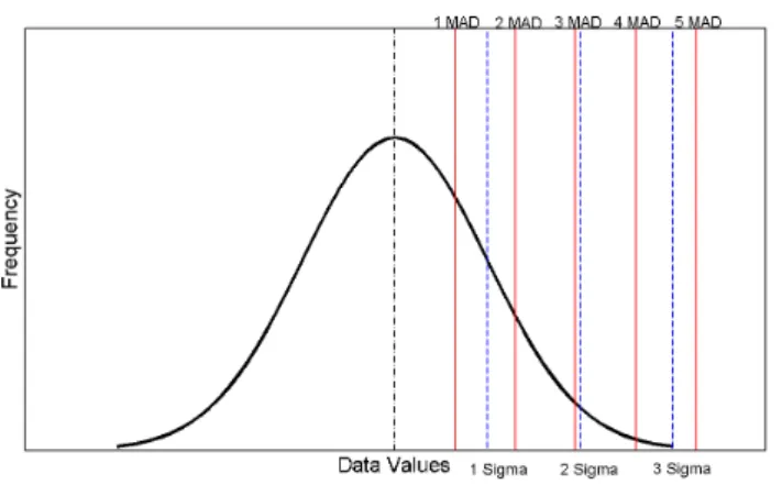
Final filtering is performed by using a statistical technique, namely the median absolute deviation (or MAD). Since a cli-matology is the most probable state of the atmosphere for a given time and location, we must be able to remove obser-vations that are considered non-representative of the most probable state. MAD is a measure of statistical dispersion and it is a powerful filtering method used to remove outliers from a sample of data (Huber, 2004). It is often preferred over the use of the standard deviation and mean of a data set as the median is considered more robust and less affected by extreme observations. Because the standard deviation is dependent upon the square of the difference from the mean value, it ensures that large deviations are heavily weighted in this calculation. When using the MAD, the magnitude of the difference between the median and a given value is less of an issue for the outlying values because of the linear re-lationship. Toohey et al. (2010) have found the MAD to be an effective method of reducing the impact of outliers when using measurements from ACE-FTS. The expression for the MAD is given in Eq. (2),
MADn=median(|xi−Mn|) (2)
Fig. 2.A random set of values can be characterized by a normal distribution curve (black thick line). The thick black dot-dash line represents the equal mean and median values for the normally dis-tributed data. The MAD values are represented by the red solid lines, while the blue dashed lines characterize the standard devia-tions.
i.e. outliers, and are therefore disregarded. For this partic-ular case, 95 % of the observations (blue stars) are retained. Since experimental data sets are not always entirely Gaussian in nature, more than 5 % of all observations will be removed by 3 MAD filtering in most cases. We find this number to be typically 5–10 % of the total population for each bin, but this still allows the data set to be representative of the atmo-spheric state.
3.3 Calculating the climatological mean values
After applying the filtering methods described above, the re-maining measurements in each bin are used to produce the climatologies. The mean value for a given bin, either latitude or equivalent latitude range, will be included in the clima-tology if there are five or more data points used in the cal-culation. This provides a level of statistical robustness in the climatological values. In making the climatologies, we cal-culate the weighted mean value within each bin using the inverse of the absolute fitting uncertainty (rather than the in-verse variance) as the weighting factor. Hence, observations with large fitting uncertainties are weighted less than those with smaller fitting uncertainties. This method is used to take the quality of the retrieved data into account when calculat-ing the climatological mean. This technique is similar to that used by Grooß and Russell (2005) in their HALOE climatol-ogy, where they weighted by the inverse of the accuracy to account for the quality of the data in their calculations.
Climatological VMR values are calculated by month and combined three-monthly climatologies are also pro-duced, namely, December-January-February (DJF), March-April-May (MAM), June-July-August (JJA), and September-October-November (SON). Note that these three-month combinations are not strictly a seasonal average. Due to the
Fig. 3.Example of January O3data (67.5◦S bin) and how outliers
are removed using MAD filtering. Red dots are data that are deemed non-representative (∼5 %) and are thus rejected. Solid black line is the median of all observations, while the dashed line is the±3 MAD envelope.Nrepresents the percentage of retained measurements af-ter 3 MAD filaf-tering (∼95 %).
SCISAT satellite’s orbit only certain latitudes/equivalent lat-itudes are measured for any given month. For some species, this can result in apparent discontinuities in the climatologi-cal values in regions where there are sharp gradients in VMR.
3.4 Additional information
To complement the climatological VMR data, we have in-cluded a suite of information to aid in the interpretation of the data set comparison. These extra data are provided as part of the climatological data products and describe the data in each bin. These data are provided on the same pressure/latitude grid (or pressure/equivalent latitude grid) as the VMR in-formation. Firstly, the standard deviation for each grid bin for each species is supplied, which will help characterize the degree of variation on a monthly (or three-monthly) basis. We also provide the number of observations for every grid bin, thus offering a measure of the level of statistical robust-ness for a given climatological value. LST information is also stored for each grid bin. These include the mean, standard deviation, median, maximum, and minimum of the LSTs for the measurements that are used to calculate the VMR clima-tological value in each grid bin.
3.5 Data formats and availability
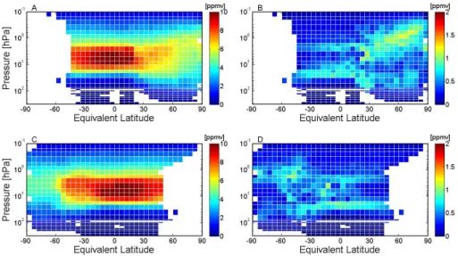
Fig. 4.ACE-FTS O3climatology for February(A)and August(C). Also shown is the one standard deviation of the O3climatology for
February(B)and August(D). The gaps in the data are either where there were no observations made (for example, the summer hemisphere pole for the months considered here) or where there are less than 5 observations for a given bin.
4 Results
The following highlights some results from the ACE-FTS cli-matologies. For brevity, we have chosen to present six of the fourteen baseline species. We have selected two radiatively important species (O3and H2O), examples of chlorine
reser-voir and source species (HCl and CCl3F) and active nitrogen
species (NO and NO2) for illustration. For O3, H2O, HCl,
and CCl3F, we provide examples of the February and
Au-gust climatological VMR fields, obtained by combining the AM + PM measurements. For NO and NO2, species which
have strong diurnal variations, we show AM and PM clima-tologies separately. Also, some examples of the three-month combined climatologies are shown. In all cases, we show the climatology calculated in terms of pressure as a function of equivalent latitude.
To ascertain a level of confidence, each of the 14 climato-logical products have been compared to various other clima-tological data sets. O3, HCl, CH4, H2O, and HF have been
compared directly to the HALOE climatology (Grooß et al., 2005), while the other species have been compared to zonal mean fields calculated from the outputs from a CCM (the Canadian Middle Atmospheric Model (CMAM), Scinocca et al., 2008) and a chemical transport model (the Global Mod-eling Initiative (GMI) combo-model driven by GEOS-4 me-teorological fields (Strahan et al., 2007). In these model com-parisons, the agreement between data sets is generally very good. When comparing the ACE-FTS and HALOE clima-tologies, we find similar biases as were found in the compar-isons of coincident ACE-FTS and HALOE measurements, as reported in the ACE validation special issue (http://www. atmos-chem-phys.org/special issue114.html). Also, we have compared our climatology results for NO2to the combined
model and measurement climatology produced by Brohede et al. (2008). These results are discussed below.
In addition, the ACE-FTS climatology has been compared with other satellite climatologies as part of the SPARC Data Initiative. The user is directed to the report from this initiative for additional comparisons and assessments (SPARC Data Initiative, in preparation).
4.1 Monthly zonal mean climatologies
O3:Figure 4 shows the monthly climatological products for ozone in February and August (panels A and C) as well as the one sigma variability for the same months respec-tively (panels B and D). The VMR values at around 10 hPa are typically greater than 10 ppmv in the tropics, while val-ues decrease gradually as one moves towards the polar lat-itudes. For these particular months, polar observations are only made in the winter. The stronger southern polar vortex (August) is more evident compared to the Northern Hemi-sphere polar vortex activity (February), which is more per-turbed (and hence weaker) due to more frequent stratospheric sudden warmings. The estimates of ozone variation are based on one standard deviation of the VMR values for each grid bin. The largest variations are found close to the peak alti-tude in VMR in the extra-tropics and polar latialti-tudes and are typically 0.5–1 ppmv. We can expect varying strengths of the polar vortex from year to year due to the relative timings of stratospheric warmings, hence we would expect to see the greatest variability in this region.
Fig. 5.Same as Fig. 4, but for H2O.
Fig. 6.Same as Fig. 4, but for CCl3F.
samples to consider then it may fail to remove (what would be considered otherwise) outliers. Although this may not af-fect the overall climatological VMR value for a given bin, it might well produce an unreliable variation value, due to the presence of an outlier(s). The total number of observations per grid cell can be used in these cases to determine the de-gree of statistical robustness.
H2O:Figure 5 illustrates the climatology for water vapour for February and August. The main photochemical source of water vapour in the stratosphere is the oxidation of CH4,
hence a typical H2O profile is anti-correlated to a typical
CH4 profile. Thus, VMRs increase with altitude
through-out the stratosphere, yielding on average maximum values of 7–8 ppmv in the upper stratosphere in the tropics. The scale for the plots in Fig. 5 were chosen to best display the stratospheric and lower mesospheric results. Because the
tro-pospheric concentrations of water vapour are significantly higher than those found in the stratosphere, the tropospheric mixing ratio values are off the scale in these plots. The very low water vapour values seen at high southern latitudes (Au-gust) are evidence of dehydration in the polar vortex. The one standard deviation climatological fields show the water vapour variation to be typically less than 0.4 ppmv through-out most of the stratosphere and lower mesosphere. Larger variation values (typically greater than 0.8 ppmv) are seen near polar latitudes and the mid-latitude/polar stratopause (∼0.1 hPa) region.
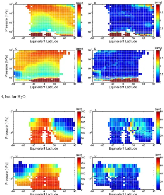
CCl3F: The ACE-FTS CCl3F distribution in the
mid-dle/upper troposphere and lowermost stratosphere is shown in Fig. 6. The CCl3F VMR values obtained range from 220–
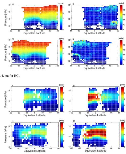
Fig. 7.Same as Fig. 4, but for HCl.
Fig. 8.NO2AM and PM climatologies for February(A)and(B)and August(C)and(D).
as CCl3F is photolysed by intense UV radiation. The
one-sigma variation values are highest in the extra-tropics in the region just above the tropopause and on the order of 30 pptv. Otherwise, variation values are typically less than 20 pptv in the troposphere and in the stratosphere.
HCl:Examples of the HCl climatology for February and August are given in Fig. 7. The stratospheric production of HCl is via the photolytic breakdown of CFCs, HCFCs, and chlorocarbons therefore HCl concentrations increase with al-titude. HCl acts as a reservoir species outside of the polar re-gions, but it is converted to its reactive form (ClO) through heterogeneous reactions on polar stratospheric clouds (PSCs) during the polar night. The breakdown of HCl is well rep-resented by the low VMR values seen in the winter polar vortex region (below 30 hPa). Background variation values are generally less than 0.2 ppbv, but around the polar
vor-tex, these variations are closer to 0.6 ppbv. The extra-tropical upper stratosphere also shows a tendency towards slightly higher variation values of about 0.4–0.5 ppb. This is likely to be related to a high bias found in the ACE-FTS HCl data at altitudes above 1 hPa. This bias has been reported in pre-vious validation studies with MLS (Froidevaux et al., 2008). NO and NO2: Both NO2 and NO, which form the NOx
family, are active nitrogen species that are important for the catalytic ozone loss cycles in the stratosphere. Both of these species have strong diurnal variations, such that they are active during sunlit hours, but are quickly locked up into reservoir species such as N2O5during the night. The strong
diurnal variation of NO2 can be seen from Fig. 8. Here,
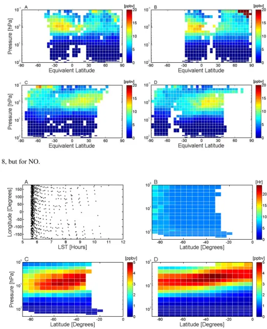
Fig. 9.Same as Fig. 8, but for NO.
Fig. 10.Spread of LST for ACE-FTS AM observations during March(A). The median LST climatological field for March(B). The ACE NO2March AM Climatology(C). The OSIRIS + model (Brohede et al., 2008) model NO2climatology (2001–2008)(D).
observations (∼4 ppbv) in the tropical middle stratosphere, the region dominated by ozone chemistry. Figure 9 uses the same format as Fig. 8 to show the NO climatology. It can be seen that PM values are slightly higher than AM in the trop-ical middle stratosphere. Moreover, it is also apparent that large abundances of NO (>20 ppbv) are descending from the winter polar mesosphere to the stratosphere, particularly in the Northern Hemisphere. These are periods typically associ-ated with solar energetic particle precipitation (EPP) (Funke et al., 2005; L´opez-Puertas et al., 2005; Rinsland et al., 2005; Randall et al., 2005, 2006, 2007; Natarajan et al., 2004). Al-though the variation plots for NO and NO2are not shown,
we have found the values to vary widely (considering AM
and PM independently), from typically less than 1 ppbv in the tropics to as large as 10–15 ppbv in EPP influenced regions.
When using the climatologies for diurnally varying species, the LST must be considered. Figure 10, panel A shows how the LST of all March NO2 AM measurements
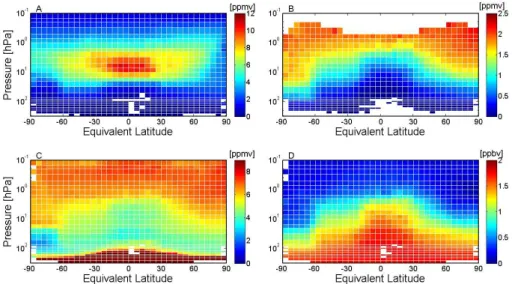
Fig. 11.ACE-FTS three-month combined climatologies (September-October-November (SON) for O3(A), for HF(B), for H2O(C), and for CH4(D).
polar latitudes are closer to 09:00 a.m. The NO2 AM
cli-matology is exhibited in panel C. We now compare the ACE-FTS NO2 zonal average to the climatology produced
by Brohede et al. (2008), who incorporated Optical Spec-trograph InfraRed Imager System (OSIRIS) measurements and results from a photochemical box model. Panel D shows the OSIRIS + model climatology data for March (2001– 2008) computed for a LST of 6 AM. Comparing panels C and D, there is a good agreement between ACE-FTS and OSIRIS + model in terms of structure and VMR val-ues. Here, differences in NO2VMRs between ACE-FTS and
OSIRIS + model are typically less than 1 ppbv, which is sim-ilar to the magnitude of bias reported in the Kerzenmacher et al. (2008) validation analysis for coincident ACE-FTS and Odin OSIRIS NO2profiles.
4.2 The 3 month combined zonal averages
Figure 11 shows an example of three-month combined zonal averages for four different species: panel A shows O3,
panel B shows HF, panel C shows H2O, and panel D shows
CH4during September-October-November (SON).
We can see that by using this methodology we can ob-tain an excellent coverage from pole to pole for these four cases. Some examples of interesting features are in panel A where there is evidence for ozone depletion in the Southern Hemisphere polar vortex, while panel C illustrates nicely the dehydration of water vapour in the Southern Hemisphere po-lar vortex. Comparison of panels C and D show the anti-correlated behaviour of H2O and CH4, where CH4 is
ox-idized to H2O as one moves up through the atmosphere.
Panel B illustrates evidence of vertical descent of enhanced HF VMRs (∼2–2.2 ppbv) from the mesospheric southern po-lar latitudes into the stratospheric popo-lar region, where HF
VMRs are less (∼1.5–1.7 ppbv). Finally, there is also evi-dence for strong horizontal mixing in the southern extra trop-ics (below∼3 hPa) seen in panel B, D, and to a lesser degree in panel C.
5 Summary
ACE-FTS profiles from the version 2.2 (plus updates for O3
and N2O5) data set have been utilized to produce multi-year
(2004–2009) zonal average climatologies for 14 atmospheric species. Monthly and combined three-month (DJF, MAM, JJA, SON) climatologies are produced on a vertical pressure grid and as a function of latitude or equivalent latitude. The ACE-FTS climatological data set contains: O3, H2O, CH4,
N2O, CO, NO, NO2, N2O5, HNO3, HCl, ClONO2, CCl3F,
CCl2F2, and HF. A statistical technique using the median
average deviation (MAD) has been employed to eliminate outliers effectively from the data set. The data quality of the retrievals (given by the inverse of the fitting error) is used to weight the values used in the climatological averages. This ACE-FTS climatology will be an excellent complement to the current climatological data sets based on measurements from other satellite missions and ozonesondes by providing data for a wider number of species in a consistent data set. These climatological products will provide a source of data for model intercomparison studies and other atmospheric re-search projects, including the SPARC initiative to evaluate climatological data sets obtained from satellite instruments (SPARC Data Initiative, in preparation).
Supplementary material related to this article is
Acknowledgements. The Atmospheric Chemistry Experiment (ACE), also known as SCISAT, is a Canadian-led mission mainly supported by the Canadian Space Agency (CSA) and the Natural Sciences and Engineering Research Council of Canada (NSERC). This work was supported by grants from the Canadian Foundation for Climate and Atmospheric Science (CFCAS) and CSA. Work at the Jet Propulsion Laboratory, California Institute of Technology is done under contract with the National Aeronautics and Space Administration. Some support is also provided by the UK Natural Environment Research Council, NERC.
Edited by: M. Dameris
References
Beaver, G. M. and Russell, J. M.: The climatology of stratospheric HCl and HF observed by HALOE, Adv. Space Res., 21, 1373– 1382, 1998.
Bernath, P. F., McElroy, C. T., Abrams, M. C., Boone, C. D., Butler, M., Camy-Peyret, C., Carleer, M., Clerbaux, C., Coheur, P. F., Colin, R., DeCola, P., Mazi`ere, M. D., Drummond, J. R., Dufour, D., Evans, W. F. J., Fast, H., Fussen, D., Gilbert, K., Jennings, D. E., Llewellyn, E. J., Lowe, R. P., Mahieu, E., McConnell, J. C., McHugh, M., McLeod, S. D., Michaud, R., Midwinter, C., Nassar, R., Nichitu, F., Nowlan, C., Rinsland, C. P., Rochon, Y. J., Rowlands, N., Semeniuk, K., Simon, P., Skelton, R., Sloan, J. J., Soucy, M. A., Strong, K., Tremblay, P., Turnbull, D., Walker, K. A., Walkty, I., Wardle, D. A., Wehrle, V., Zander, R., and Zou, J.: Atmospheric Chemistry Experiment (ACE): Mission overview, Geophys. Res. Lett., 32, L15S01, doi:10.1029/2005GL022386, 2005.
Boone, C. D., Nassar, R., Walker, K. A., Rochon, Y. J., McLeod, S. D., Rinsland, C. P., and Bernath, P. F.: Retrievals for the Atmo-spheric Chemistry Experiment Fourier-Transform Spectrometer, Appl. Optics, 44, 7218–7231, 2005.
Brohede, S., McLinden, C. A., Urban, J., Haley, C. S., Jonsson, A. I., and Murtagh, D.: Odin stratospheric proxy NOy
mea-surements and climatology, Atmos. Chem. Phys., 8, 5731–5754, doi:10.5194/acp-8-5731-2008, 2008.
Butchart, N. and Remsberg, E. E.: The area of the stratospheric po-lar vortex as a diagnostic for tracer transport on an isentropic surface, J. Atmos. Sci., 43, 1319–1339, 1986.
Carleer, M. R., Boone, C. D., Walker, K. A., Bernath, P. F., Strong, K., Sica, R. J., Randall, C. E., V¨omel, H., Kar, J., H¨opfner, M., Milz, M., von Clarmann, T., Kivi, R., Valverde-Canossa, J., Sioris, C. E., Izawa, M. R. M., Dupuy, E., McElroy, C. T., Drummond, J. R., Nowlan, C. R., Zou, J., Nichitiu, F., Los-sow, S., Urban, J., Murtagh, D., and Dufour, D. G.: Validation of water vapour profiles from the Atmospheric Chemistry Ex-periment (ACE), Atmos. Chem. Phys. Discuss., 8, 4499–4559, doi:10.5194/acpd-8-4499-2008, 2008.
Chiou, E. W., McCormick, M., and Chu, W. P.: Global water vapor distributions in the stratosphere and upper troposphere derived from 5.5 years of SAGE II observations (1986–1991), J. Geo-phys. Res., 102, 19105–19118, 1997.
Clerbaux, C., George, M., Turquety, S., Walker, K. A., Barret, B., Bernath, P., Boone, C., Borsdorff, T., Cammas, J. P., Catoire, V.,
Coffey, M., Coheur, P.-F., Deeter, M., De Mazi`ere, M., Drum-mond, J., Duchatelet, P., Dupuy, E., de Zafra, R., Eddounia, F., Edwards, D. P., Emmons, L., Funke, B., Gille, J., Griffith, D. W. T., Hannigan, J., Hase, F., H¨opfner, M., Jones, N., Ka-gawa, A., Kasai, Y., Kramer, I., Le Flochmo¨en, E., Livesey, N. J., L´opez-Puertas, M., Luo, M., Mahieu, E., Murtagh, D., N´ed´elec, P., Pazmino, A., Pumphrey, H., Ricaud, P., Rinsland, C. P., Robert, C., Schneider, M., Senten, C., Stiller, G., Strandberg, A., Strong, K., Sussmann, R., Thouret, V., Urban, J., and Wiacek, A.: CO measurements from the ACE-FTS satellite instrument: data analysis and validation using ground-based, airborne and spaceborne observations, Atmos. Chem. Phys., 8, 2569–2594, doi:10.5194/acp-8-2569-2008, 2008.
Dupuy, E., Walker, K. A., Kar, J., Boone, C. D., McElroy, C. T., Bernath, P. F., Drummond, J. R., Skelton, R., McLeod, S. D., Hughes, R. C., Nowlan, C. R., Dufour, D. G., Zou, J., Nichi-tiu, F., Strong, K., Baron, P., Bevilacqua, R. M., Blumenstock, T., Bodeker, G. E., Borsdorff, T., Bourassa, A. E., Bovens-mann, H., Boyd, I. S., Bracher, A., Brogniez, C., Burrows, J. P., Catoire, V., Ceccherini, S., Chabrillat, S., Christensen, T., Cof-fey, M. T., Cortesi, U., Davies, J., De Clercq, C., Degenstein, D. A., De Mazi`ere, M., Demoulin, P., Dodion, J., Firanski, B., Fischer, H., Forbes, G., Froidevaux, L., Fussen, D., Gerard, P., Godin-Beekmann, S., Goutail, F., Granville, J., Griffith, D., Ha-ley, C. S., Hannigan, J. W., H¨opfner, M., Jin, J. J., Jones, A., Jones, N. B., Jucks, K., Kagawa, A., Kasai, Y., Kerzenmacher, T. E., Kleinb¨ohl, A., Klekociuk, A. R., Kramer, I., K¨ullmann, H., Kuttippurath, J., Kyr¨ol¨a, E., Lambert, J.-C., Livesey, N. J., Llewellyn, E. J., Lloyd, N. D., Mahieu, E., Manney, G. L., Mar-shall, B. T., McConnell, J. C., McCormick, M. P., McDermid, I. S., McHugh, M., McLinden, C. A., Mellqvist, J., Mizutani, K., Murayama, Y., Murtagh, D. P., Oelhaf, H., Parrish, A., Petelina, S. V., Piccolo, C., Pommereau, J.-P., Randall, C. E., Robert, C., Roth, C., Schneider, M., Senten, C., Steck, T., Strandberg, A., Strawbridge, K. B., Sussmann, R., Swart, D. P. J., Tarasick, D. W., Taylor, J. R., T´etard, C., Thomason, L. W., Thompson, A. M., Tully, M. B., Urban, J., Vanhellemont, F., Vigouroux, C., von Clarmann, T., von der Gathen, P., von Savigny, C., Waters, J. W., Witte, J. C., Wolff, M., and Zawodny, J. M.: Validation of ozone measurements from the Atmospheric Chemistry Experi-ment (ACE), Atmos. Chem. Phys., 9, 287–343, doi:10.5194/acp-9-287-2009, 2009.
Fortuin, J. P. F. and Kelder, H.: An ozone climatology based on ozonesonde and satellite measurements, J. Geophys. Res., 103, 31709–31734, 1998.
Froidevaux, L., Jiang, Y. B., Lambert, A., Livesey, N. J., Read, W. G., Waters, J. W., Fuller, R. A., Marcy, T. P., Popp, P. J., Gao, R. S., Fahey, D. W., Jucks, K. W., Stachnik, R. A., Toon, G. C., Christensen, L .E., Webster, C. R., Bernath, P .F., Boone, C. D., Walker, K. A., Pumphrey, H. C., Harwood, R. S., Manney, G. L., Schwartz, M. J., Daffer, W. H., Drouin, B. J., Cofield, R. E., Cuddy, D. T., Jarnot, R. F., Knosp, B. W., Perun, V. S., Snyder, W. V., Stek, P. C., Thurstans, R. P. and Wagner, P. A.: Validation of Aura Microwave Limb Sounder HCl measurements, J. Geophys. Res., 113, D15S25, doi:10.1029/2007JD009025, 2008. Funke, B., L´opez-Puertas, M., Gil-L`opez, S., von Clarmann,
Arctic 2002/2003 winters, J. Geophys. Res., 110, D09308, doi:10.1029/2005JD006463, 2005.
Gilbert, K.L.,Turnbull, D. N., Walker, K. A., Boone, C. D., McLeod, S. D., Butler, M., Skelton, R., Bernath, P. F., Chateauneuf, F., and Soucy, M. A.: The onboard imagers for the Cana-dian ACE SCISAT-1 mission, J. Geophys. Res., 112, D12207, doi:10.1029/2006JD007714, 2007.
Grooß, J.-U. and Russell III, J. M.: Technical note: A stratospheric climatology for O3, H2O, CH4, NOx, HCl and HF derived from
HALOE measurements, Atmos. Chem. Phys., 5, 2797–2807, doi:10.5194/acp-5-2797-2005, 2005.
Hoffmann, L., Kaufmann, M., Spang, R., Muller, R., Remedios, J. J., Moore, C., Volk, M., and von Clarmann, T.: Envisat MIPAS measurements of CFC-11: retrieval, validation, and climatology, Atmos. Chem. Phys., 8, 3671–3688, 2008,
http://www.atmos-chem-phys.net/8/3671/2008/. Huber, P.: Robust Statistics, Wiley, New York, 2004.
Jones, A., Qin, G., Strong, K., Walker, K. A., McLinden, C. A., Toohey, M., Kerzenmacher, T., Bernath, P. F., and Boone, C. D.: A global inventory of stratospheric NOyfrom ACE-FTS, J.
Geo-phys. Res., 116, D17304, doi:10.1029/2010JD015465, 2011. Kerzenmacher, T., Wolff, M. A., Strong, K., Dupuy, E., Walker, K.
A., Amekudzi, L. K., Batchelor, R. L., Bernath, P. F., Berthet, G., Blumenstock, T., Boone, C. D., Bramstedt, K., Brogniez, C., Brohede, S., Burrows, J. P., Catoire, V., Dodion, J., Drummond, J. R., Dufour, D. G., Funke, B., Fussen, D., Goutail, F., Grif-fith, D. W. T., Haley, C. S., Hendrick, F., H¨opfner, M., Huret, N., Jones, N., Kar, J., Kramer, I., Llewellyn, E. J., L´opez-Puertas, M., Manney, G., McElroy, C. T., McLinden, C. A., Melo, S., Mikuteit, S., Murtagh, D., Nichitiu, F., Notholt, J., Nowlan, C., Piccolo, C., Pommereau, J.-P., Randall, C., Raspollini, P., Ri-dolfi, M., Richter, A., Schneider, M., Schrems, O., Silicani, M., Stiller, G. P., Taylor, J., T´etard, C., Toohey, M., Vanhellemont, F., Warneke, T., Zawodny, J. M., and Zou, J.: Validation of NO2and
NO from the Atmospheric Chemistry Experiment (ACE), At-mos. Chem. Phys., 8, 5801–5841, doi:10.5194/acp-8-5801-2008, 2008.
Kouker, W., Langbein, I., Reddmann, T., and Ruhnke, R.: The Karl-sruhe simulation model of the middle atmosphere (KASIMA), version 2, 6278, FZKA Wissenschaftliche Berichte – Scientific Reports, Forschungszentrum Karlsruhe, 1999.
L´opez-Puertas, M., Funke, B., Gil-L´opez, S., Von Clarmann, T., Stiller, G. P., H¨opfner, M., Kellman, S., Fischer, H., and Jack-man, C. H.: Observation of NOx enhancement and ozone
de-pletion in the Northern and Southern Hemispheres after the October-November 2003 solar proton events, J. Geophys. Res., 110, A09S43, doi:10.1029/2005JA011050, 2005.
Mahieu, E., Duchatelet, P., Demoulin, P., Walker, K. A., Dupuy, E., Froidevaux, L., Randall, C., Catoire, V., Strong, K., Boone, C. D., Bernath, P. F., Blavier, J.-F., Blumenstock, T., Coffey, M., De Mazi`ere, M., Griffith, D., Hannigan, J., Hase, F., Jones, N., Jucks, K. W., Kagawa, A., Kasai, Y., Mebarki, Y., Mikuteit, S., Nassar, R., Notholt, J., Rinsland, C. P., Robert, C., Schrems, O., Senten, C., Smale, D., Taylor, J., T´etard, C., Toon, G. C., Warneke, T., Wood, S. W., Zander, R., and Servais, C.: Validation of ACE-FTS v2.2 measurements of HCl, HF, CCl3F and CCl2F2using
space-, balloon- and ground-based instrument observations, At-mos. Chem. Phys., 8, 6199–6221, doi:10.5194/acp-8-6199-2008, 2008.
Manney, G. L., Daffer, W. H., Zawodny, J. M., Bernath, P. F., Hop-pel, K. W., Walker, K. A., Knosp, B. W., Boone, C., Remsberg, E. E., Santee, M. L., Lynn Harvey, V., Pawson, S., Jackson, D. R., Deaver, L., McElroy, C. T., McLinden, C. A., Drummond, J. A., Pumphrey, H. C., Lambert, A., Schwartz, M. J., Froidevaux, L., McLeod, S., Takacs, L. L., Suarez, M. J., Trepte, C. R., Cuddy, D. T., Livesey, N. J., Harwood, R. S., and Waters, J. W.: Solar Occultation Satellite Data and Derived Meteorological Products: Sampling Issues and Comparisons with Aura MLS, J. Geophys. Res., 112, D24S50, doi:10.1029/2007JD008709, 2007. De Mazi`ere, M., Vigouroux, C., Bernath, P. F., Baron, P.,
Blu-menstock, T., Boone, C., Brogniez, C., Catoire, V., Coffey, M., Duchatelet, P., Griffith, D., Hannigan, J., Kasai, Y., Kramer, I., Jones, N., Mahieu, E., Manney, G. L., Piccolo, C., Randall, C., Robert, C., Senten, C., Strong, K., Taylor, J., T´etard, C., Walker, K. A., and Wood, S.: Validation of ACE-FTS v2.2 methane pro-files from the upper troposphere to the lower mesosphere, At-mos. Chem. Phys., 8, 2421–2435, doi:10.5194/acp-8-2421-2008, 2008.
McElroy, C. T., Nowlan, C. R., Drummond, J. R., Bernath, P. F., Barton, D. V., Dufour, D. G., Midwinter, C., Hall, R. B., Ogyu, A., Ullberg, A., Wardle, D. I., Kar, J., Zou, J., Nichitiu, F., Boone, C. D., Walker, K. A., and Rowlands, N.: The ACE-MAESTRO instrument on SCISAT: Description, performance, and prelimi-nary results, Appl. Optics, 46, 4341–4356, 2007.
McLinden, C. A., Olsen, S. C., Hannegan, B., Wild, O., Prather, M. J., and Sundet, J.: Stratospheric ozone in 3-D models: A simple chemistry and the cross-tropopause flux, J. Geophys. Res., 105, 14653–14665, 2000.
McLinden, C. A., Haley, C. S., and Sioris, C. E.: Diurnal effects in limb scatter observations, J. Geophys. Res., 111, D14302, doi:10.1029/2005JD006628, 2006.
McPeters, R. D., Labow, G. J., and Logan, J. A.: Ozone climatolog-ical profiles for satellite retrieval algorithms, J. Geosphys Res., 112, D05308, doi:10.1029/2005JD006823, 2007.
Nassar, R., Bernath, P. F., Boone, C. D., McLeod, S. D., Skel-ton, R., Walker, K. A., Rinsland, C. P., and Duchatelet, P.: A global inventory of stratospheric fluorine in 2004 based on At-mospheric Chemistry Experiment Fourier transform spectrome-ter (ACE-FTS) measurements, J. Geophys. Res., 111, D22313, doi:10.1029/2006JD007395, 2006.
Natarajan, M., Remsberg, E. E., Deaver, E. E., and Russell III, J. M.: Anomalously high levels of NOx in the polar
up-per stratosphere during Apr, 2004: Photochemical consistency of HALOE observations, Geophys. Res. Lett. 31, L15113, doi:10.1029/2004GL020566, 2004.
Randall, C. E., Harvey, V. L., Manney, G. L., Orsolini, Y., Codrescu, M., Sioris, C., Brohede, S., Haley, C. S., Gordley, L. L., Za-wodny, J. M., and Russell, J. M.: Stratospheric effects of ener-getic particle precipitation in 2003–2004, Geophys. Res. Lett., 32, L05802, doi:10.1029/2004GL022003, 2005.
Randall, C. E., Harvey, V. L., Singleton, C. S., Bernath, P. F., Boone, C. D., and Kozyra, J. U.: Enhanced NOx in 2006 linked to
strong upper stratospheric Arctic vortex, Geophys. Res. Lett., 33, L18811, doi:10.1029/2006GL027160, 2006.
doi:10.1029/2006JD007696, 2007.
Randel, W. J., Wu, F., Russell, J. M., Roche, A., and Waters, J. W.: Seasonal cycles and QBO variations in stratospheric CH4 and H2O observed in UARS HALOE data, J. Atmos. Sci., 55, 163–
185, 1998.
Rienecker, M. M., Suarez, M. J., Todling, R., Bacmeister, J., Takacs, L., Liu, H.-C., Gu, W., Sienkiewicz, M., Koster, R. D., Gelaro, R., Stajner, I., and Nielsen, J. E.: The GEOS-5 Data Assimila-tion System – DocumentaAssimila-tion of Versions 5.0.1, 5.1.0, and 5.2.0, Technical Report Series on Global Modeling and Data Assimila-tion, 27, 2008.
Rinsland, C. P., Boone, C., Nassar, R., Walker, K., Bernath, P., Mc-Connell, J. C., and Chiou, L.: Atmospheric Chemistry Experi-ment (ACE) Arctic stratospheric measureExperi-ments of NOxduring
February and March 2004: Impact of intense solar flares, Geo-phys. Res. Lett., 32, L16S05, doi:10.1029/2005GL022425, 2005. Rothman, L. S., Jacquemart, D., Barbe, A., Chris Bennerc, D., Birk, M., Brown, L. R., Carleer, M. R., Chackerian Jr., C., Chance, K., Coudert, L. H., Dana, V., Devi, V. M., Flaud, J.-M., Gamache, R. R., Goldman, A., Hartmann, J.-M., Jucks, K. W., Maki, A. G., Mandin, J.-Y., Massie, S. T., Orphal, J., Perrin, A., Rinsland, C. P., Smith, M. A. H., Tennyson, J., Tolchenov, R. N., Toth, R. A., Vander Auwera, J., Varanasi, P., and Wagner, G.: The HITRAN 2004 molecular spectroscopic database, J. Quant. Spectrosc. Ra., 96, 139–204, 2005.
Russell, J. M., Gordley, L. L., Park, J. H., Drayson, S. R., Tuck, A. F., Harries, J. E., Cicerone, R. J., Crutzen, P. J., and Frederick, J. E.: The Halogen Occultation Experiment, J. Geophys. Res., 98, 10777–10797, 1993.
Scinocca, J. F., McFarlane, N. A., Lazare, M., Li, J., and Plummer, D.: Technical Note: The CCCma third generation AGCM and its extension into the middle atmosphere, Atmos. Chem. Phys., 8, 7055–7074, doi:10.5194/acp-8-7055-2008, 2008.
SPARC CCMVal, SPARC Report on the Evaluation of Chemistry-Climate Models, edited by: Eyring, V., Shepherd, T. G., and Waugh, D. W., SPARC Report No. 5, WCRP-132, WMO/TD-No. 1526, 2010.
SPARC Data Initiative, SPARC Data Initiative Report, edited by: Hegglin, M. I. and Tegtmeier, S., SPARC Report No. 6, in prepa-ration.
Strong, K., Wolff, M. A., Kerzenmacher, T. E., Walker, K. A., Bernath, P. F., Blumenstock, T., Boone, C., Catoire, V., Coffey, M., De Mazi`ere, M., Demoulin, P., Duchatelet, P., Dupuy, E., Hannigan, J., H¨opfner, M., Glatthor, N., Griffith, D. W. T., Jin, J. J., Jones, N., Jucks, K., Kuellmann, H., Kuttippurath, J., Lam-bert, A., Mahieu, E., McConnell, J. C., Mellqvist, J., Mikuteit, S., Murtagh, D. P., Notholt, J., Piccolo, C., Raspollini, P., Ri-dolfi, M., Robert, C., Schneider, M., Schrems, O., Semeniuk, K., Senten, C., Stiller, G. P., Strandberg, A., Taylor, J., T´etard, C., Toohey, M., Urban, J., Warneke, T., and Wood, S.: Validation of ACE-FTS N2O measurements, Atmos. Chem. Phys., 8, 4759–
4786, doi:10.5194/acp-8-4759-2008, 2008.
Strahan, S. E., Duncan, B. N., and Hoor, P.: Observationally de-rived transport diagnostics for the lowermost stratosphere and their application to the GMI chemistry and transport model, At-mos. Chem. Phys., 7, 2435–2445, doi:10.5194/acp-7-2435-2007, 2007.
Toohey, M., Strong, K., Bernath, P. F., Boone, C. D., Walker, K. A., Jonsson, A. I., and Shepherd, T. G.: Validating the reported ran-dom errors of ACE?FTS measurements, J. Geophys. Res., 115, D20304, doi:10.1029/2010JD014185, 2010.
Urban, J., Pommier, M., Murtagh, D. P., Santee, M. L., and Orsolini, Y. J.: Nitric acid in the stratosphere based on Odin observations from 2001 to 2009 – Part 1: A global climatology, Atmos. Chem. Phys., 9, 7031–7044, doi:10.5194/acp-9-7031-2009, 2009. Wolff, M. A., Kerzenmacher, T., Strong, K., Walker, K. A., Toohey,