Estimating the influence of the secondary organic aerosols on present climate using ECHAM5-HAM

(1)

ACPD

11, 2407–2472, 2011

Estimating the influence of the secondary organic

aerosols

D. O’Donnell et al.

Title Page

Abstract Introduction

Conclusions References

Tables Figures

◭ ◮

Back Close

Full Screen / Esc

Printer-friendly Version Interactive Discussion

Discussion

P

a

per

|

Dis

cussion

P

a

per

|

Discussion

P

a

per

|

Discussio

n

P

a

per

|

Atmos. Chem. Phys. Discuss., 11, 2407–2472, 2011 www.atmos-chem-phys-discuss.net/11/2407/2011/ doi:10.5194/acpd-11-2407-2011

Atmospheric Chemistry and Physics Discussions

This discussion paper is/has been under review for the journal Atmospheric Chemistry and Physics (ACP). Please refer to the corresponding final paper in ACP if available.

Estimating the influence of the secondary

organic aerosols on present climate using

ECHAM5-HAM

D. O’Donnell1,*, K. Tsigaridis2,**, and J. Feichter1,*

1

Max Planck Institute for Meteorology, Bundesstrasse 55, 20146 Hamburg, Germany

2

Laboratoire des Sciences du Climat et de l’Environnement (LSCE), 91191 Gif-sur-Yvette, France

*

now at: Institute for Atmospheric Science and Climate, ETH Z ürich, Universit ätstrasse 16, 8092 Z ürich, Switzerland

**

now at: Center for Climate System Research, Columbia University and NASA Goddard Institute for Space Studies, 2880 Broadway, New York NY10025, USA

Received: 20 December 2010 – Accepted: 3 January 2011 – Published: 24 January 2011 Correspondence to: D. O’Donnell (declan.odonnell@env.ethz.ch)

(2)

ACPD

11, 2407–2472, 2011

aerosols

Title Page

Tables Figures

◭ ◮

Back Close

Full Screen / Esc

Discussion

P

a

per

|

Dis

cussion

P

a

per

|

Discussion

P

a

per

|

Discussio

n

P

a

per

|

Abstract

In recent years, several field measurement campaigns have highlighted the importance of the organic fraction of aerosol mass, and with such spatial diversity that one may as-sert that these aerosols are ubiquitous in the troposphere, with particular importance in continental areas. Investigation of the chemical composition of organic aerosol re-5

mains a work in progress, but it is now clear that a significant portion of the total or-ganic mass is composed of secondary oror-ganic material, that is, aerosol chemically formed from gaseous volatile organic carbon (VOC) precursors. A number of such precursors, of both biogenic and anthropogenic origin, have been identified. Exper-imental, inventory building and modelling studies have followed. Laboratory studies 10

have yielded information on the chemical pathways that lead to secondary organic aerosol (SOA) formation, and provided the means to estimate the aerosol yields from a given precursor-oxidant reaction. Global inventories of anthropogenic VOC emis-sions, and of biogenic VOC emitter species distribution and their emission potential have been constructed. Models have been developed that provide global estimates of 15

precursor VOC emissions, SOA formation and atmospheric burdens of these species. This paper estimates the direct and indirect e_ffects of these aerosols using the global climate-aerosol model ECHAM5-HAM. For year 2000 conditions, we estimate a global annual mean shortwave (SW) aerosol direct effect due to SOA of −0.3 W m−2. The model predicts a positive SW indirect e_ffect due to SOA amounting to ₊0.23 W m−2, 20

(3)

ACPD

11, 2407–2472, 2011

aerosols

Title Page

Tables Figures

◭ ◮

Back Close

Full Screen / Esc

Discussion

P

a

per

|

Dis

cussion

P

a

per

|

Discussion

P

a

per

|

Discussio

n

P

a

per

|

1 Introduction

Organic aerosols constitute an important part of the tropospheric aerosol loading. In regions affected by anthropogenic pollution, organic species have been observed to be the second most abundant component by mass after sulphate, and frequently the most important contributor to aerosol light scattering (Hegg et al., 1997; Novakov et al., 5

1997; Ramanathan et al., 2001). In tropical forested areas, it forms the dominant part of the aerosol mass (Andreae and Crutzen, 1997; Artaxo et al., 1988, 2002), even in the absence of large-scale biomass burning. Organic aerosols are found in the remote marine environment (Middlebrook et al., 1998), in the free troposphere (Huebert et al., 2004; Heald et al., 2005) and in the upper troposphere (Murphy et al., 1998; Froyd et 10

al., 2009).

Organic aerosol may be formed by direct emission into the atmosphere in the particle phase (primary organic aerosols, POA) or by condensation into the particle phase of organic species created by the oxidation of a gas-phase precursor (secondary organic aerosol, SOA). Both biogenic and anthropogenic precursors are known. Estimates 15

of global emissions of precursors of biogenic (Guenther et al., 1995, 2006) and of anthropogenic (van Aardenne et al., 2005) precursors indicate that biogenic emissions (of the order of hundreds of Tg/yr) are an order of magnitude greater than those of known anthropogenic precursors.

Furthermore, some measurements show a concentration of organic aerosol that is 20

well above that predicted by the current generation of global aerosol-climate models (Heald et al., 2005; Volkamer et al., 2006). Most such models include only POA or include SOA in a very simple, implicit treatment, for example the AEROCOM approach (Dentener et al., 2006), in which SOA is considered to be formed in fixed proportion to prescribed monoterpene emissions in each grid box, and to have identical properties 25

to (and therefore possible to lump together with) POA.

(4)

ACPD

11, 2407–2472, 2011

aerosols

Title Page

Tables Figures

◭ ◮

Back Close

Full Screen / Esc

Discussion

P

a

per

|

Dis

cussion

P

a

per

|

Discussion

P

a

per

|

Discussio

n

P

a

per

|

such aerosols in isolation. Chung and Seinfeld (2002), considering only biogenic pre-cursors, estimated a global annual mean SOA burden of 0.19 Tg from a production of 11.2 Tg/yr. Tsigaridis and Kanakidou (2003) included anthropogenic aromatic precur-sors (not including benzene, not known at that time to be a significant SOA precursor) in a sensitivity study that attempted to constrain SOA production and atmospheric bur-5

den, estimating the production bounds to be 2.5–44.5 Tg/yr. These studies exclude isoprene, since they predate the discovery that isoprene can be a significant source of SOA. Henze and Seinfeld (2006) first included SOA from isoprene in a global study, with the result that SOA production almost doubled and the SOA burden more than doubled (to 16.4 Tg/yr and 0.39 Tg, respectively) compared with the same model with-10

out SOA from isoprene. Hoyle et al. (2007), although using isoprene emissions lower than other models, estimated SOA production of 55–69 Tg/yr and a SOA burden of 0.52–0.70 Tg in the global annual mean. Hoyle et al. (2009), using an offline radiative transfer model, and assuming an external aerosol mixture, estimated the radiative forc-ing (present day minus preindustrial) of anthropogenic SOA to be−0.06–−0.09 W m−2. 15

In this study, we examine how the aerosol direct effect and indirect effects are af-fected by secondary organic aerosols using the aerosol-climate model ECHAM5/HAM (Stier at al., 2005), which has been extended to handle SOA. This allows us to deploy a model with online radiation and cloud microphysics that are coupled to an aerosol population which is resolved in both aerosol size distribution and mixing state. Both 20

particle size distribution and mixing state are important for the calculation of radiative properties, and at least the size distribution is important for aerosol indirect effects (Stier et al., 2005).

2 Model description

The model upon which this study is based is ECHAM5/HAM, described and evaluated 25

(5)

ACPD

11, 2407–2472, 2011

aerosols

Title Page

Tables Figures

◭ ◮

Back Close

Full Screen / Esc

Discussion

P

a

per

|

Dis

cussion

P

a

per

|

Discussion

P

a

per

|

Discussio

n

P

a

per

|

is referred to the works cited above.

ECHAM5/HAM is a modal model that describes the aerosol population as a super-position of seven lognormal modes. For each mode, aerosol mass and number con-centrations are prognostic variables. Four of these modes are termed “soluble”, which means, in the context of this model, that the particles are internally mixed and may 5

take up water. Soluble modes cover the size ranges 1–10 nm (nucleation mode), 10– 100 nm (Aitken mode), 100 nm–1 µm (accumulation mode) and>1 µm (coarse mode) dry particle diameter. Insoluble modes do not take up water, are regarded as exter-nally mixed and cover Aitken, accumulation and coarse modes. The modelled aerosol species are sulphate, black carbon, organic carbon, sea salt and mineral dust. In the 10

original model version, “organic carbon” refers to POA plus SOA formed by assum-ing a fixed 15% SOA yield from the monoterpene emissions estimates of Guenther et al. (1995), with immediate non-volatile SOA production in the emitting gridbox. This ap-proach is no longer used. Modelled processes include emission, aerosol microphysics (water uptake, condensation of SO₄from the gas phase, new particle nucleation, and 15

coagulation), sink processes (wet deposition, dry deposition and sedimentation) and cloud droplet activation. Cloud droplet number concentration (CDNC) and ice crystal number concentration (ICNC) are calculated as functions of the aerosol size distribu-tion and possibly composidistribu-tion, depending on the activadistribu-tion scheme chosen. The model includes a simple sulphate chemistry scheme, for which prescribed monthly mean oxi-20

dant concentrations with a superimposed diurnal cycle are used.

A SOA scheme, described in the following sections, has been added to this model. The aim is to keep this scheme as simple and computationally cost-effective as possible while capturing the most significant known SOA sources.

2.1 Emission of SOA precursors 25

(6)

ACPD

11, 2407–2472, 2011

aerosols

Title Page

Tables Figures

◭ ◮

Back Close

Full Screen / Esc

Discussion

P

a

per

|

Dis

cussion

P

a

per

|

Discussion

P

a

per

|

Discussio

n

P

a

per

|

Emission of biogenic species is calculated online in the model using MEGAN (Guen-ther et al. 2006; Guen(Guen-ther, 2007) for isoprene and the earlier work of (Guen(Guen-ther et al., 1995) for monoterpenes. No distinction is made between different monoterpene species: α-pinene is used as a surrogate for all monoterpenes. Isoprene emission is calculated using the parameterised canopy environment emission activity (PCEEA) 5

approach of the MEGAN model. Leaf age and soil moisture are not taken into account in this implementation. Leaf area index (LAI) is prescribed, varying monthly. Emissions of monoterpenes then depend on temperature and LAI only and those of isoprene on temperature, LAI and photosynthetically active radiation. Note that in the formulations provided by these parameterisations, “temperature” means leaf temperature. This is 10

not available in ECHAM5/HAM; instead the lowest model level temperature is used. Emission of anthropogenic species is according to the EDGAR fast-track 2000 is-sue, hereafter FT2000, (van Aardenne et al., 2005). The FT2000 issue does not pro-vide explicit speciation of the emitted volatile organic compounds (VOC), in contrast to the 1990 issue. We assume that the species mix is identical in both. For each 15

gridpoint, the fraction of total VOC that each included species makes up is calculated from the 1990 dataset and applied in turn to the FT2000 dataset to obtain the year 2000 estimate. We model SOA production from toluene, xylene and benzene. The 1990 dataset also includes emissions of trimethylbenzene and a group labeled “other aromatics”. Trimethylbenzene is a known SOA precursor and is lumped together with 20

xylene. 50% of the “other aromatics” are also included in this class. No information is available on the diurnal or seasonal variation of anthropogenic VOC emission on a global basis, so emissions are treated as constant in time.

Precursors only exist in the gas phase in the model.

2.2 Formation of SOA

25

(7)

ACPD

11, 2407–2472, 2011

aerosols

Title Page

Tables Figures

◭ ◮

Back Close

Full Screen / Esc

Discussion

P

a

per

|

Dis

cussion

P

a

per

|

Discussion

P

a

per

|

Discussio

n

P

a

per

|

(OH in the case of isoprene and anthropogenics and O₃in the case of monoterpenes) are considered to produce SOA.

A drawback of this approach is that the known dependency of SOA yield on ambient NO_x (Presto et al., 2005; Kroll et al., 2006; Ng et al., 2007b) is lacking in the model. The entire atmosphere is treated as low-NO_x, a point to which we shall return in the 5

discussion of the model results.

The two-product model of SOA formation is used. This model is founded on the work of Odum and colleagues (Odum et al., 1996), who showed that for a reaction yielding many semi-volatile species, the aerosol yieldY, defined as

Y= ∆M

∆HC (1)

10

where_∆M is the change in aerosol mass and _∆HC is the mass of precursor hydro-carbon consumed, can be modelled by assuming that the reaction produces only two condensable species. In this approach, the gas-phase reaction of a precursor PRE and oxidant OX resulting in the two hypothetical productsP₁andP₂is described by

PRE+OX→α₁P₁+α₂P₂ (2)

15

where α₁ and α₂ are mass-based stoichiometric coe_fficients, and subsequent gas-aerosol partitioning by

Ai=Kp,iM0Gi (3)

where A_i (i=1, 2) denotes the mass of product P_i that resides in the aerosol phase andGi in the gas phase,Kp,i is apartitioning coefficientfor the organic mass, andM0

20

is the total SOA-absorbing mass in the aerosol phase. SOA production is then fully characterised by the four empirical parametersα₁,α₂,K_p,₁andK_p,₂.

Ng et al. (2007a) found that in the case of low NO_x, SOA formed from xylene, toluene and benzene is effectively non-volatile. This allows us to represent the SOA yield from these precursors in terms of a single product species that, after formation, condenses 25

(8)

ACPD

11, 2407–2472, 2011

aerosols

Title Page

Tables Figures

◭ ◮

Back Close

Full Screen / Esc

Discussion

P

a

per

|

Dis

cussion

P

a

per

|

Discussion

P

a

per

|

Discussio

n

P

a

per

|

The chosen two-product parameters and reaction rates for this model are given in Table 1.

Oxidant concentrations are prescribed as in Stier et al. (2005), except that NO₃ is added using the multi-model mean computed for year 2000 by the RETRO re-analysis project (http://retro.enes.org/index.shtml). The constancy of the oxidant fields over 5

each model timestep makes the system simple enough to solve analytically. 2.3 SOA gas-aerosol partitioning

Equation (3) describes only the partitioning between the gas phase mass and the total aerosol phase SOA mass. In our model, this is not su_fficient since we must determine the mass that partitions to each of the size-resolved modes. Firstly, we must consider 10

what is meant by the termM₀ in Eq. (3). The underlying theory developed by Pankow (1994a,b) is based on absorption and notadsorption. This means that SOA must be able to partition into the bulk of the material considered as absorber, not just attach to surface sites. For this reason, we exclude black carbon, mineral dust and crystalline salts as SOA absorbers. Note, however, that in ECHAM5/HAM, “sulphate” encom-15

passes more than just salts; in particular it includes sulphuric acid. In the light of the effect of seed particle acidity on SOA discussed by Iinuma et al. (2004), and findings of organosulphates in aerosol (Surratt et al., 2007), this suggests that sulphate may play a role in determining the gas-aerosol partitioning of SOA; however, all such identified mechanisms are chemical and not purely thermodynamic mechanisms, which means 20

that they cannot be quantified through the Pankow theoretical framework.

Perhaps a more intractable question concerns SOA and aerosol water. Many SOA species are to some degree water-soluble and SOA is (usually weakly) hygroscopic. So one may pose the question: does water take up SOA or does SOA take up water? The answer may of course be “both”. However, since, in most regions, water uptake is 25

(9)

ACPD

11, 2407–2472, 2011

aerosols

Title Page

Tables Figures

◭ ◮

Back Close

Full Screen / Esc

Discussion

P

a

per

|

Dis

cussion

P

a

per

|

Discussion

P

a

per

|

Discussio

n

P

a

per

|

uptake of all SOA species by all SOA species and by primary organics.

Pankow (1994a) derived an expression for the partitioning coe_fficientK_p,i in terms of temperature and aerosol solution properties, here presented in the slightly modified form of Seinfeld and Pankow (2003), and in terms of SI units:

K_p_,i= RT

MW_OMζip0_i

(4) 5

where MW_OM is the mean molecular weight of the organic aerosol, R the universal gas constant, T the temperature, ζ_i the activity coefficient of compound i and p0_i its saturation vapour pressure. We take the activity coefficient of each compound to be unity. The Clausius-Clapeyron equation for the temperature dependence ofp0_i applied to (4) then allows us to calculate K_p_,i at any temperature from that at a reference 10

temperatureTref, where the partitioning coefficient is (Kp,i)ref:

K_p,i= Kp,i_ref T T_refexp

_∆_H

i R

₁

T − 1 T_ref

(5)

where∆Hi is the enthalpy of vaporisation of compoundi.∆Hi is set to 42 kJ/mol for all semivolatile species in this model.

In this model, SOA partitioning is calculated independently of SOA formation. SOA 15

is transported and can evaporate or condense as ambient conditions vary.

WhereSi is the total mass of semi-volatile SOA speciesi, andAi andGi its aerosol and gas phase masses, respectively, then

S_i=A_i+G_i (6)

Substituting from Eq. (3) and rearranging gives 20

G_i= Si

1₊K_p,iM0

(10)

ACPD

11, 2407–2472, 2011

aerosols

Title Page

Tables Figures

◭ ◮

Back Close

Full Screen / Esc

Discussion

P

a

per

|

Dis

cussion

P

a

per

|

Discussion

P

a

per

|

Discussio

n

P

a

per

|

and Ai=

Kp,iM0Si 1+Kp,iM0

(8)

Thus the SOA absorbing massM0must be known before the partitioning can be

calcu-lated, although it is itself a function of the SOA aerosol mass. Recalling thatM₀consists of a non-volatile partM_NV(which in this model consists of POA and non-volatile SOA), 5

plus all condensed SOA, M₀=M_NV+X

i

Ai (9)

Substituting from Eq. (8), we have finally

M₀=M_NV+M₀ n X

i=1

K_p_,iS_i 1₊K_p,iM0

(10)

Thus, since the total non-volatile and semi-volatile massesM_NVandS_i are known, we 10

can computeM0 and thence the gas and aerosol phase masses of the semi-volatile

species.

So far, we have presented nothing new with respect to SOA partitioning and Eq. (10) and the foregoing equations have been stated in many previous works (e.g., Seinfeld and Pankow, 2003; Tsigaridis and Kanakidou, 2003; Hoyle et al., 2007).

15

We now come to the question of how SOA partitions between aerosols of different size classes. Repeating the derivation of Pankow (1994a,b), under the assumption that there exists a partitioning coe_fficientK_p,i,j for speciesi in each modej, results in a similar expression to Eq. (4)

K_p,i,j=

RT MW_OM_,jζi ,jp0_i

(11)

ACPD

11, 2407–2472, 2011

aerosols

Title Page

Tables Figures

◭ ◮

Back Close

Full Screen / Esc

Discussion

P

a

per

|

Dis

cussion

P

a

per

|

Discussion

P

a

per

|

Discussio

n

P

a

per

|

where MW_OM_,j is the mean molecular weight of the organic species in modej, andζ_{i ,j} the activity coe_fficient for species i the mode. The ratio of mode to bulk partitioning coe_fficient is then

K_p_,i,j K_p_,i =

MW_OMζi

MW_OM_,jζ_{i ,j} (12)

Since the activity coefficients are taken to be unity for all modes, only the ratio of the 5

mean molecular weights remains, for which unity is a reasonable assumption. Then the bulk partitioning coe_fficient can be used for all modes.

It is shown in the Appendix that the neglect of the activity coefficientζ_i is consistent with a SOA partitioning between di_fferent size classes according to the fraction of non-volatile absorbing aerosol mass in each mode. That is, if M_NV and A_i are the total 10

non-volatile absorbing mass and the total aerosol phase mass of theith SOA species, andMNVj andAi j the respective quantities in modej, then

A_{i j} Ai =

M_NV_j MNV

(13) For each semi-volatile species, the prognostic quantity in the model is the total con-densable SOA mass (S_i). For non-volatile organics, it is the mass per mode (M_NV_j). 15

At the beginning of the gridpoint physics routines, we diagnose the total semi-volatile aerosol and gas phase masses according to Eqs. (7) and (8). The semi-volatile mass per mode is then calculated from Eq. (13).

Hence in the model SOA partitions strongly in favour of the larger modes. Equa-tion (13) has particular consequences for the impact of SOA on cloud condensaEqua-tion 20

nuclei (CCN): since these are larger particles, SOA preferentially condenses on parti-cles that are already of CCN size.

(12)

ACPD

11, 2407–2472, 2011

aerosols

Title Page

Tables Figures

◭ ◮

Back Close

Full Screen / Esc

Discussion

P

a

per

|

Dis

cussion

P

a

per

|

Discussion

P

a

per

|

Discussio

n

P

a

per

|

Thermodynamic data (such as enthalpy of adsorption) that would permit one to calcu-late adsorptive partitioning do not exist.

2.4 Measuring model SOA production and lifetime

For semi-volatile species, it is not obvious how to measure the quantitySOA production, since the aerosol mass changes in response to ambient conditions. We can, nonethe-5

less, estimate this quantity for semi-volatile species in another way. While the total net condensation flux is not directly available from the equilibrium partitioning scheme, we do know the total sink flux. On the assumption of source-sink aerosol mass bal-ance over a model integration period, (in which one may have some confidence, if not proof, if the total semi-volatile budget is balanced for the species in question), then the 10

production term may be assumed to be the same as the sum of the sink terms.

Themodel lifetime τ_M of semi-volatile species in the aerosol phase can be defined as the ratio of the mean aerosol burdenB(t) to the integrated production (sink) flux:

τ_M= 1 T2−T1

T₂ R

T₁

B(t)d t

T2

R

T₁

F↓_{(t)d t}

(14)

whereF↓(t) is the sum of the spatially-integrated sink terms, and the model integration 15

runs from timeT₁toT₂. Clearly,τ_Mis applicable only as a global total metric. 2.5 Aerosol water uptake

The original ECHAM5/HAM water uptake scheme is that of Jacobson et al. (1996), which models water uptake by electrolytic species. In order to take into account uptake of water by organics, the semi-empirical scheme of Petters and Kreidenweis (2007) 20

(13)

ACPD

11, 2407–2472, 2011

aerosols

Title Page

Tables Figures

◭ ◮

Back Close

Full Screen / Esc

Discussion

P

a

per

|

Dis

cussion

P

a

per

|

Discussion

P

a

per

|

Discussio

n

P

a

per

|

of only a single free parameter κ). For sulphate, sea salt and organic species, the appropriate mean growth factor (GF) derivedκ value found in Petters and Kreidenweis (2007) is used.

The overall internally mixed aerosolκ is the volume-weighted sum (over the soluble fraction, i.e. in the soluble modes only, and excluding any black carbon and dust) of the 5

individual compoundκ values, as per Eq. (7) in Petters and Kreidenweis (2007). The growth factor can then be calculated using Eq. (11) in that paper,viz.

RHexp

− A

D_dgf

= gf 3₋₁

gf3−(1−κ) (15)

wheregf is the growth factor, RH the relative humidity (in thecloud-freefraction of the gridbox) on the fractional scale,D_dis the particle dry diameter andAis the Kelvin term 10

A=4σs/aMw

RTρ_w (16)

whereσ_s/ais the surface tension of water (0.072 Jm−2) (note that any surface tension effect of the solutes are encapsulated in theκ parameter),Mwis the molecular weight

of water andρ_w its density. In this implementation, to minimise computational costs, Eq. (15) is solved offline forgf as a function ofT, RH,D_d andκand the results stored 15

in a lookup table. OnceDd and κ have been calculated for each mode, we can then

simply look up the growth factor (interpolation to the lookup table values is linear inT, RH andκ, and linear in the logarithm ofD_d).

2.6 Sink processes for SOA

SOA is subject to wet deposition, dry deposition and sedimentation (Stier et al. 2005) 20

(14)

ACPD

11, 2407–2472, 2011

aerosols

Title Page

Tables Figures

◭ ◮

Back Close

Full Screen / Esc

Discussion

P

a

per

|

Dis

cussion

P

a

per

|

Discussion

P

a

per

|

Discussio

n

P

a

per

|

2.7 SOA and cloud processes

In the simulations described herein, cloud droplet activation is calculated according to the scheme of Lin and Leaitch (1997), in which only the aerosol size, not its compo-sition, is taken into account. Thus in the model, SOA a_ffects cloud droplet number only through its effect on particle size, not through hygroscopicity, nor by affecting the 5

surface tension of droplets. Clouds affect SOA through the above-described wet sink processes.

No aqueous-phase SOA chemistry is included.

3 Model results

The simulations described herein are simulations of the year 2000. The model dynam-10

ics are calculated in spectral space with triangular truncation at term 63 (T63), while physics are calculated on a 1.8◦×1.8◦ Gaussian grid. The simulations use 31 vertical levels, from the surface to 10 hPa. The model diagnostics are output every 6 simu-lated hours. Large-scale meteorology is constrained by nudging towards the ECMWF analysis for the year 2000.

15

Three simulations were performed: one without SOA, one with SOA and one with only biogenic SOA. The results of the latter are very similar to those of the simulation with all SOA, and in the following we will describe the results in terms of the simulations without SOA and with all SOA. Where results of the simulation with biogenic SOA only are presented, this is specifically mentioned.

20

3.1 SOA precursor emissions

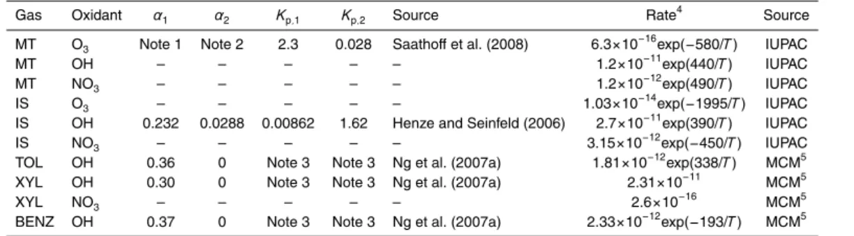
The annual emission flux of each anthropogenic precursor is shown in Fig. 1.

(15)

ACPD

11, 2407–2472, 2011

aerosols

Title Page

Tables Figures

◭ ◮

Back Close

Full Screen / Esc

Discussion

P

a

per

|

Dis

cussion

P

a

per

|

Discussion

P

a

per

|

Discussio

n

P

a

per

|

regulated in the United States and Europe; it has greatest emission in South and East Asia.

Mean wintertime and summertime emissions of isoprene and monoterpenes are shown in Fig. 2. Observe that different scales are used for isoprene and for penes. Global annual totals are calculated as 446 Tg/yr isoprene and 89 Tg/yr monoter-5

penes. This compares with a figure of 17 Tg/yr for the sum of the anthropogenic pre-cursors (6 Tg/yr toluene, 6 Tg/yr xylene and 5 Tg/yr benzene).

Biogenic emissions are predominantly tropical, with more than 75% (on an annu-alised basis) of biogenics originating from these latitudes. Boreal forest emissions are significant in the summer months, but weak in wintertime.

10

3.2 SOA budget

The model SOA mass budget is presented in Table 2.

Anthropogenic precursor emissions having no diurnal or seasonal variation in the model, the seasonal variability in anthropogenic SOA production is, as one would intu-itively expect, rather limited, with monthly global total production varying from 0.42 to 15

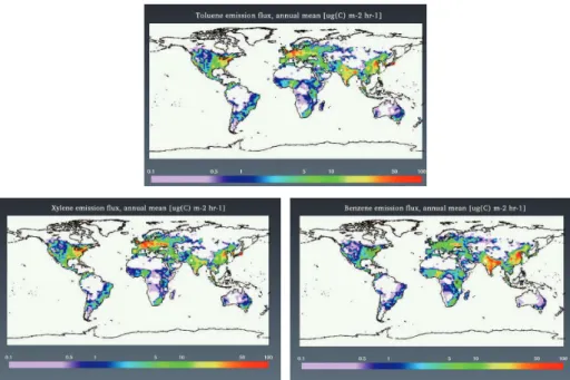
0.50 Tg/month. The global maximum production takes place in Northern Hemisphere (NH) spring. This is due to a precursor reservoir that is built up at high latitudes during the winter, when the photochemical sink is weak. Europe, the United States, Japan, China and India are the main source regions for anthropogenic SOA. Annual anthro-pogenic SOA production, vertically integrated over the atmospheric column, is shown 20

in Fig. 4.

Production of biogenic SOA species, since these are semi-volatile, is only possible to estimate as a global total according to the methodology of Sect. 2.4. This gives estimates of 17 Tg/yr and 4.0 Tg/yr aerosol from isoprene and monoterpenes, respec-tively. Together with the estimated 5.6 Tg/yr from anthropogenic precursors, this gives 25

(16)

ACPD

11, 2407–2472, 2011

aerosols

Title Page

Tables Figures

◭ ◮

Back Close

Full Screen / Esc

Discussion

P

a

per

|

Dis

cussion

P

a

per

|

Discussion

P

a

per

|

Discussio

n

P

a

per

|

For the non-volatile species, the sink fluxes are in much the same ratios as for pri-mary OC, with wet deposition removing over 90% of the aerosol mass from the atmo-sphere. One may note that despite the a_ffinity of SOA for larger aerosol particles in the model, sedimentation remains a very weak sink for organic mass. This is especially so for the biogenic species, most likely because they are semi-volatile and evaporate in 5

warm near-surface conditions.

For semi-volatile SOA formed from isoprene and monoterpenes, the largest sinks are directly from the gas phase.

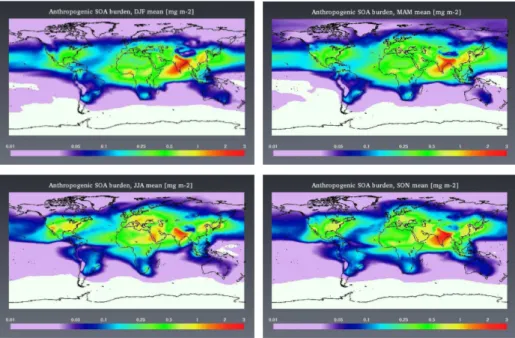
The modelled seasonal mean anthropogenic and biogenic SOA burdens are shown in Figs. 3 and 4, respectively.

10

It is notable that the model isoprene-derived SOA burden exceeds that of SOA from monoterpenes and anthropogenic precursors by an order of magnitude, a ratio consid-erably greater than that between the estimated respective aerosol production fluxes, and that its estimated lifetime is also much larger. This is due to the particular vertical distribution of model isoprene SOA, which is discussed in Sect. 3.4.

15

3.3 Geographical and seasonal distribution of SOA

A combination of high emissions and active photochemistry gives a high anthropogenic SOA burden over South and Southeast Asia, weakening in the summer with the en-hancement of the wet deposition sink. Low wintertime OH levels north of 45◦N lead to very little SOA formation despite substantial precursor emissions from Europe and the 20

North-Eastern United States.

The biogenic SOA loading is strongly dominated by the contribution of tropical forests, with a comparatively small (on an annualised basis) input from the Boreal forest. The peak in September–November in the Amazon is related to the biomass burning season. SOA formation is related to the amount of organic absorbing material 25

(17)

ACPD

11, 2407–2472, 2011

aerosols

Title Page

Tables Figures

◭ ◮

Back Close

Full Screen / Esc

Discussion

P

a

per

|

Dis

cussion

P

a

per

|

Discussion

P

a

per

|

Discussio

n

P

a

per

|

that are not accounted for in the model. Elsewhere, the “biogenic hotspot” in the South-Eastern United States is clearly visible in the summer months. Also worth remarking upon is the relatively low burden over the forests of Indonesia and Papua New Guinea, despite the high precursor emissions in those areas. Heavy model precipitation in that region e_fficiently removes SOA through wet deposition.

5

3.4 Vertical distribution of SOA

Vertical transport plays a crucial role in SOA formation. Convection lifts gas-phase condensable species to much colder regions of the atmosphere, where partitioning favours the aerosol phase. The common occurrence of deep convection in the trop-ics thus enhances SOA formation, already favoured due to high precursor emissions 10

and strong photochemistry. Kulmala et al. (2006) suggested a similar mechanism for insoluble organics.

The simulation without SOA, with values of less than 5 ng m−3 above 8 km, cannot explain observations of organic aerosols (Murphy et al., 1998; Froyd et al., 2009; Mor-gan et al., 2009) in the upper troposphere. The annual zonal mean of total orMor-ganic 15

aerosol mass is presented in Fig. 5.

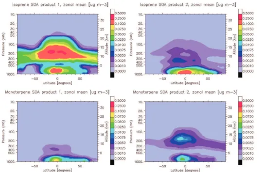
The two-product model of SOA formation is clearly visible in the modelled vertical profile of biogenic SOA (Fig. 6). For each modelled biogenic precursor, we have two SOA products of differing volatilities. The more volatile products require lower temper-atures for the gas-aerosol partitioning to favour the aerosol phase. The split is clearly 20

visible in the vertical profile, which is shown in Fig. 6 as the annual zonal mean con-centration for each semi-volatile product. In reality, SOA is composed of a range of compounds of differing volatilities, so that the two peaks of the model distribution is unlikely to be an accurate reflection of true vertical distribution.

A high-altitude SOA pool is formed mainly in the tropical mid- to upper troposphere at 25

(18)

ACPD

11, 2407–2472, 2011

aerosols

Title Page

Tables Figures

◭ ◮

Back Close

Full Screen / Esc

Discussion

P

a

per

|

Dis

cussion

P

a

per

|

Discussion

P

a

per

|

Discussio

n

P

a

per

|

The high upper-tropospheric loading of isoprene-derived SOA requires close exam-ination. It comes about as a result of the two-product properties of isoprene-derived SOA, in particular those of product 1, for which the laboratory data chosen (Henze and Seinfeld, 2006) gives a stoichiometric yield of 0.232 and a partitioning coefficient of 0.00862 m3/µg at 295 K. The former implies an input to the atmosphere (assuming 5

OH supply is non-limiting) of some 100 Tg/yr condensable gas from the model iso-prene emissions of 446 Tg/yr. The latter implies that the compound so formed is highly volatile and favours the gas phase down to very low temperatures (K_p=1 m3/µg at 228 K for an absorbing mass ofM₀=1 µg/m3). The combination of high yield and high volatil-ity results in an aerosol species that condenses primarily in the upper troposphere, at 10

temperatures too cold for liquid water. The high altitude and lack of wet removal (SOA in the model does not interact with ice) lead to the high modelled burden and extended lifetime.

3.5 Impact of SOA on aerosol number concentration

Since SOA condenses onto pre-existing aerosol, one would intuitively expect that the 15

main effect of SOA on aerosol number is to boost some of the population of the smaller modes into the larger size ranges. This is indeed so in the zonal and annual mean: in particular, the soluble accumulation mode number concentration is increased at the expense of the soluble Aitken mode. The zonal mean number concentrations of these modes are shown in Figs. 7 and 8, respectively. Numbers are also enhanced in the 20

coarse mode, though the e_ffect is rather small compared to the accumulation mode. The increase in the number of larger particles enhances the coagulation sink of small particles.

Number concentrations in the nucleation and Aitken modes are depleted in the sim-ulation with SOA compared to that without SOA. For the nucleation mode (which in the 25

(19)

ACPD

11, 2407–2472, 2011

aerosols

Title Page

Tables Figures

◭ ◮

Back Close

Full Screen / Esc

Discussion

P

a

per

|

Dis

cussion

P

a

per

|

Discussion

P

a

per

|

Discussio

n

P

a

per

|

soluble by condensation of sulphuric acid and by coagulation with the soluble modes, and hence generally confined to the lower and mid-troposphere. The influence of SOA on this mode is also minor.

3.6 Aerosol optical properties

The model global annual mean aerosol optical depth at 550 nm is 0.13, compared to 5

0.12 without SOA. The annual mean AOD is shown in Fig. 9. Seasonal and regional variations in the AOD difference follow the variations of the SOA burden, as discussed in Sect. 3.5, reaching a local maximum of about 0.2 in the Amazonian basin in the biomass burning season.

3.7 Direct and indirect effects of SOA 10

Finally, we present the modelled influence of SOA upon climate in terms of radiative effects. We do not attempt to estimate the radiativeforcing in terms of present minus preindustrial climate, since the biogenic emissions model requires a gridded dataset of emission factors, that depend on the vegetation present in the grid cell, and which is available only for present-day conditions. An estimate of the radiative forcing due to 15

SOA requires that changes in land cover, especially tropical deforestation, are taken into account, which is beyond the present capabilities of this model. Instead, we esti-mate the directeffect as the difference in the top of the atmosphere (ToA) net radiative flux under clear-sky conditions between a simulation including SOA and a simulation with zero SOA, with the large-scale meteorology constrained by nudging as described 20

in the introduction to Sect. 3. The indirect effect is the difference in the TOA fluxes under cloudy (all-sky minus clear-sky) conditions.

The direct e_ffect is shown in Fig. 10. On the global annual mean, it amounts to a cool-ing of−0.31 W m−2, with peak cooling of approximately−2 W m−2in the southwest of the Amazon basin, where the Andes form a barrier (compare the maximum annual 25

(20)

ACPD

11, 2407–2472, 2011

aerosols

Title Page

Tables Figures

◭ ◮

Back Close

Full Screen / Esc

Discussion

P

a

per

|

Dis

cussion

P

a

per

|

Discussion

P

a

per

|

Discussio

n

P

a

per

|

Antarctica. These are connected with the changes in the particle diameter towards the larger size range, which is most pronounced in these regions. Larger particles scatter more radiation in the forward direction, and thus less radiation is lost to space than would be the case with the same number of smaller particles of identical composition. Elsewhere, it is noteworthy that the boreal forest contributes significantly only in the 5

Northern Hemisphere summer (not shown) and little in the annual mean. The biogenic SOA only simulation gives a clear-sky effect of−0.29 W m−2.

The model gives a noisy result for the SOA indirect effect (Fig. 11). For this reason, Fig. 11 has been subject to a 9-point smoothing algorithm. The result is somewhat surprising, in that the modelled indirect effect of SOA is clearly positive in some re-10

gions: North-Western Europe, especially the North Sea, Japan and the surrounding maritime area, much of South America and the West African coast from approximately the equator to 20◦S.

This is related to seasonal perturbations of stratus decks in anthropogenically influ-enced (whether by industry or biomass burning) areas. The mechanism appears to be 15

as follows: in the model, the Lin and Leaitch activation scheme is used, whereby any particle with radius of at least 35 nm can act as a cloud condensation nucleus (CCN). In this model scheme, SOA partitions preferentially to large particles (thus, to those that are already of CCN size). Therefore, in the model, SOA in the polluted areas leads to an increase in the radius of CCN-sized particles without increasing their number, thus 20

opposing the first indirect e_ffect. In the presence of a su_fficient number of larger parti-cles, the condensable SOA supply is essentially exhausted by those partiparti-cles, leaving very little growth “fuel” for small particles, while at the same time enhancing the coag-ulation sink for the small particles. The net result is adecreasein CCN. On the other hand, if there are few large particles available, SOA will drive growth of small particles 25

and this can result in anincreasein CCN.

(21)

ACPD

11, 2407–2472, 2011

aerosols

Title Page

Tables Figures

◭ ◮

Back Close

Full Screen / Esc

Discussion

P

a

per

|

Dis

cussion

P

a

per

|

Discussion

P

a

per

|

Discussio

n

P

a

per

|

present. Stratiform cloud decks often cover only a single model level. In the NH winter, a reduction in CDNC can be seen over Europe and parts of China; in the NH summer, a smaller reduction can be seen over Japan and offthe West African coast.

Globally, the modelled global mean SOA indirect effect is a warming of+0.23 W m−2. Whether this e_ffect should be classified as a feedback of natural aerosols or as an 5

anthropogenic forcing requires some reflection. Since it is a short-term response gen-erated by the presence of large numbers of anthropogenic particles, the latter is prob-ably more appropriate. However, for the purposes of calculating an overall e_ffect of SOA, it will be treated as a feedback.

Longwave (thermal) radiative effects are small, a global clear-sky total of 10

+0.02 W m−2, and an indirect e_ffect of−0.03 W m−2.

Assuming additivity of these effects, the overall model estimate of the climate impact of SOA under year 2000 conditions is therefore−0.09 W m−2.

4 Model evaluation

4.1 Comparison with measurements

15

For evaluation of global aerosol-climate models, measurements of modelled species over wide areas and long time intervals are desirable. Unfortunately, few such data sets are available as far as organic species are concerned, and none that explicitly provides SOA data. Long-term and wide-area measurements are almost invariably clustered in economically advanced countries. In view of the importance of tropical 20

regions to the model, this situation is not optimal. However, lacking better alternatives, in this section, we compare measurements of organic carbon (OC) aerosol mass taken in Europe and the United States against model values calculated at the same points.

When one considers semi-volatile species, because of the sensitivity of SOA parti-tioning to temperature, measurements must necessarily be made at ambient temper-25

(22)

ACPD

11, 2407–2472, 2011

aerosols

Title Page

Tables Figures

◭ ◮

Back Close

Full Screen / Esc

Discussion

P

a

per

|

Dis

cussion

P

a

per

|

Discussion

P

a

per

|

Discussio

n

P

a

per

|

upper troposphere, such measurements must be made in-situ and not, for example, by collection on filters and subsequent ground-level analysis. Unfortunately, such mea-surements that can explicitly give organic mass (rather than, for example, an organic to sulphate mass ratio, e.g., Froyd et al., 2009) are scarce. Some information about the performance of the updated model in the whole atmospheric column may be obtained 5

from optical measurements. To this end the Aeronet (Holben et al., 1998) network of measurement sites is used.

The biogenic emission model is evaluated in the work of Guenther et al. (1995, 2006) and this work is not repeated here.

All measurements are quoted in mass of organic aerosol (not mass of organic car-10

bon).

4.1.1 North America

The IMPROVE (InteragencyMonitoringProtectedVisualEnvironments) network (http: //vista.cira.colostate.edu/improve/) has recorded aerosol properties over the contigu-ous United States since the 1980s, and, as its mission is primarily to monitor visibility 15

at places of outstanding natural beauty, it is a rural network. The network measure-ment dataset has been analysed for the same period (namely July 2002–June 2003) that covers the European EMEP EC/OC campaign, which is analysed in the following section. The IMPROVE observations of OC for this period consists of a total of 1915 monthly mean observations from circa 160 stations (not all stations reported during 20

each month of this period). For comparison, the model was run for the same time period (after spinup), nudged to ECMWF analysis, with and without SOA.

The quoted IMPROVE measurements are for PM₂_.₅.

The distributions of observed and modelled OC mass are presented in Fig. 14 as frequency of observed/modelled mass in bins of 0.5 µg/m3.

25

(23)

ACPD

11, 2407–2472, 2011

aerosols

Title Page

Tables Figures

◭ ◮

Back Close

Full Screen / Esc

Discussion

P

a

per

|

Dis

cussion

P

a

per

|

Discussion

P

a

per

|

Discussio

n

P

a

per

|

1.46 µg/m3observed, 0.36 µg/m3modelled without SOA and 0.64 µg/m3with SOA. Wildfires are, episodically, a major factor in aerosol loading at some of the IMPROVE stations (observations of organic carbon are as high as 57 µg/m3in the monthly mean in the study period). Real fire events are not always present in the model, and in such cases very large differences between model and observations occur. Another conse-5

quence is that the standard deviations of these datasets are very large. These factors destroy any overall correlation between the observations and modelled data. Also, while some improvement in agreement on the large scale between model and obser-vations is visible from Fig. 15, it is notable that the obserobser-vations remain consistently higher than modelled OC concentrations, particularly in winter time.

10

The distribution of IMPROVE observations exhibits a single peak near 1 µg/m3. Clearly, the simulation with SOA better approaches the observed distribution: however, the occurrence of low total POM is still much higher in the model than in observations.

4.1.2 Europe

A one-year-long measurement campaign (called the EC/OC campaign) was carried 15

out by the European Monitoring and Evaulation Programme (EMEP) from July 2002– June 2003. Twelve stations participated in the campaign. One station (Kosetice, Czech Republic) did not report data for the first two months of the campaign, giving a total of 142 monthly mean observations.

The EC/OC campaign results document PM₁₀ measurements only. This is poten-20

tially important, since the model is not designed to include large particles, as those particles are less radiatively active and have short atmospheric lifetimes (recall that the coarse mode in the model consists of a lognormal distribution of particles larger than 1 µm diameter). A sample containing a significant proportion of OC mass in particles of the uppermost size range of PM₁₀ is therefore not possible to capture with the model. 25

(24)

ACPD

11, 2407–2472, 2011

aerosols

Title Page

Tables Figures

◭ ◮

Back Close

Full Screen / Esc

Discussion

P

a

per

|

Dis

cussion

P

a

per

|

Discussion

P

a

per

|

Discussio

n

P

a

per

|

While the inclusion of SOA increases the total modelled organic mass substantially (by 50% on the average of all sites for the year in question), in general the modelled mass remains well short of the measured OC mass. Only at one site (Kollumerwaard, Netherlands) and for three out of twelve months does the modelled mass equal or exceed the measured mass, and this is the case only for the simulation with SOA. This 5

difference between model and observations is particularly large in the more southerly sites in wintertime, when the large organic peaks observed at Ispra, ISAC Belogna (Italy) and Braganca (Portugal), sites that are located at latitudes between 42◦N and 46◦N, are absent in the model.

Overall, the mean of all OC mass measurements at all stations in the EMEP EC/OC 10

campaign is 3.85 µg/m3, compared to 0.90 µg/m3 modelled (without SOA) at the grid-boxes containing the relevant stations, and 1.35 µg/m3 modelled with SOA. The re-spective median values are 3.49 µg/m3 observed, 0.69 µg/m3 modelled without SOA and 1.13 µg/m3with SOA.

The model capture of seasonal variation may be measured by the correlation be-15

tween model and measurements. For Europe this is, as a whole, poor: only 0.42 for the full measurement dataset (without SOA) and even poorer, 0.39, with SOA. Exclud-ing the three Southern European stations at Bracanga, Ispra and ISAC leaves better agreement of the variation of model and observations, with a correlation of 0.70 be-tween observations and model without SOA and 0.75 with SOA. The mean of the 20

observations excluding these stations is 3.1 µg/m3, compared with modelled values of 1.0 µg/m3 (without SOA) and 1.4 µg/m3(with SOA). On this basis, the model seems to reflect the seasonal variation in total OC reasonably well in the Northern and Central Europe, even though the magnitude remains short of the measurements. In the south, however, the model differs by up to an order of magnitude to observed OC values. In 25

addition, it is temporally anti-correlated to observations in that region.

(25)

ACPD

11, 2407–2472, 2011

aerosols

Title Page

Tables Figures

◭ ◮

Back Close

Full Screen / Esc

Discussion

P

a

per

|

Dis

cussion

P

a

per

|

Discussion

P

a

per

|

Discussio

n

P

a

per

|

three southern sites, 0.95. This indicates that the OC content is largely anthropogenic throughout the campaign domain, and almost exclusively so in the south.

4.1.3 Aeronet

Aeronet observations over the period of the EMEP EC/OC campaign comprises a total of 845 monthly mean observations at locations spread worldwide (but not uniformly, 5

so that, for example, aeronet means are not comparable to satellite-derived global means). Aeronet observations include aerosol optical depth (AOD) measurements at different wavelengths. The wavelengths measured depend upon the measuring site, but measurements at 500 nm and 875 nm are commonly available. The model diag-nostic AOD is calculated at 550 nm and 825 nm, so that although we are not comparing 10

identical quantities, they can be expected to be very closely related. The distribution of measured and modelled mid-visible AOD at the aeronet sites is shown in Fig. 16.

The incidence of very low (less that 0.05) mid-visible AOD in the model is reduced by about 20% in the simulation with SOA compared to that without SOA, but low AOD remains much more common in the model than in the aeronet observations. Otherwise, 15

the distribution is moved slightly in the direction of higher AOD. Overall, the relevant mean (median) values are 0.225 (0.169) observed, 0.125 (0.103) for the model without SOA, and 0.149 (0.120) for the model with SOA.

Results for the near-infrared AOD are broadly similar, with a reduction in the inci-dence of modelled low AOD and increase in that of high AOD.

20

For the near-infrared, the relevant mean (median) AOD values are 0.117 (0.088) observed, 0.082 (0.067) for the model without SOA, and 0.094 (0.077) for the model with SOA.

With the inclusion of SOA, the correlation between Aeronet observations and model increases marginally, from 0.71 to 0.73 for the mid-visible AOD, and from 0.66 to 0.67 25

for the near-infrared AOD.

(26)

ACPD

11, 2407–2472, 2011

aerosols

Title Page

Tables Figures

◭ ◮

Back Close

Full Screen / Esc

Discussion

P

a

per

|

Dis

cussion

P

a

per

|

Discussion

P

a

per

|

Discussio

n

P

a

per

|

4.2 Comparison with other models

Due to the importance of isoprene to the results, this model inter-comparison is limited to those studies which include isoprene as a SOA precursor. In Table 3, the emissions, production and burdens calculated by previous studies and this study are listed. Emis-sions of isoprene, monoterpenes and anthropogenics are denotedE_i, E_t and E_a and 5

are given in Tg(C)/yr. Production and burdens of the respective species are denoted P_i,P_t, P_a, B_i, B_t and B_a, and the total SOA burden by B_tot. Production figures are in Tg/yr and burden figures in Tg unless otherwise stated.

The ostensibly good agreement in total SOA burden between the models belies the wide di_fferences in SOA production and in burdens of individual species, and any such 10

agreement must therefore be regarded as coincidental. Production figures must be viewed with caution, since, as discussed in Sect. 2.4, the definition of “SOA produc-tion” is not clear when applied to semi-volatile species, and none of the studies listed specifies how exactly the model in question calculates this diagnostic. There are sub-stantial differences between the model choices of SOA production pathways. For ex-15

ample, Hoyle et al. (2007), following Chung and Seinfeld (2002), assume unity mass yield of SOA from all monoterpenes under NO₃oxidation (usingβ-pinene as surrogate species), whereas the study of Tsigaridis and Kanakidou (2007) and this study as-sume zero SOA yield for this case (usingα-pinene as surrogate species). Both these approaches are valid, based on the selection of the surrogate species (Ho_ffman et 20

al., 1997).

Other key di_fferences include the nature of the models: all models in the listed stud-ies except this study include full chemistry models with prognostic OH, O₃ and NO₃, compared to the highly simplified scheme and prescribed oxidant values in this model. This study is the only one of those listed that uses a size-resolved aerosol model with 25

(27)

ACPD

11, 2407–2472, 2011

aerosols

Title Page

Tables Figures

◭ ◮

Back Close

Full Screen / Esc

Discussion

P

a

per

|

Dis

cussion

P

a

per

|

Discussion

P

a

per

|

Discussio

n

P

a

per

|

Hoyle et al. (2007) and Henze et al. (2008) simulated the year 2004, but using diff er-ent meteorological datasets. The two online models, Heald et al. (2008) and this study, both simulated the year 2000. The consequent meteorological di_fferences between the models can lead to variations in emissions (of biogenic precursors), in SOA formation, in convective and advective transport, and in sink processes.

5

The models also di_ffer in resolution in both the horizontal and the vertical. This gives rise to differences in numerical diffusion between models, which causes further variation in the transport of aerosols and gases.

5 Discussion

5.1 Emissions

10

Biogenic emissions calculated by the model lie within the range of other models, which have been evaluated against observations. This, however, must be viewed with cau-tion. Firstly, MEGAN and its predecessors, especially Guenther et al. (1995), underlie most global biogenic emission models, and therefore a comparison of ostensibly diff er-ent models is to a large exter-ent comprised of a comparison of different implementations 15

of the same underlying parameterisation. This can give one the illusion that estimates of global biogenic emissions are well-constrained, when this is not the case. This subject is analysed in more detail by Arneth et al. (2008), who point out that global es-timates of biogenic emissions remain poorly constrained, despite the seeming agree-ment among models.

20

Anthropogenic emissions are derived by assuming that the mix of different species in 2000 is the same as that for 1990. Technological and regulatory changes during the intervening period may have altered the mix. Perhaps more importantly, seasonality is lacking in the emissions for primary organic particles as well as for anthropogenic SOA precursors. Other reasons may include lack of wood burning emissions, which 25

(28)

ACPD

11, 2407–2472, 2011

aerosols

Title Page

Tables Figures

◭ ◮

Back Close

Full Screen / Esc

Discussion

P

a

per

|

Dis

cussion

P

a

per

|

Discussion

P

a

per

|

Discussio

n

P

a

per

|

(Simpson et al., 2007). This may play an important role in reconciling the model with observations over, for example, Southern Europe in wintertime.

5.2 SOA production

5.2.1 SOA precursors

There are known SOA precursors, both biogenic and anthropogenic, that are not in-5

cluded in the model. These include methyl chavicol and sesquiterpenes, emissions of which remain unquantified. The latter class of compounds may be important in new particle nucleation: this is further discussed by Bonn et al. (2003, 2008). Furthermore, they have high molecular weight, and are known to have a high aerosol mass yield (Lee et al., 2006).

10

Several anthropogenic substances that can yield SOA are known, but not included in the model either for lack of emissions estimates, or because they are recent discover-ies. It has long been known that alkanes can yield aerosol, but this has been observed for larger (in terms of carbon number) members of the alkanes group: EDGAR emis-sions estimates are given only for the group as a whole. Certain alkenes are also SOA 15

precursors (Forstner et al., 1997; Kalberer et al., 2000). A recent discovery is that even the lightest non-methane hydrocarbon (acetylene, C₂H₂) can yield SOA (Volkamer et al., 2009). These compounds may go some way to explaining the large discrepancy between modelled and measured OC in anthropogenically-dominated regions.

5.2.2 SOA in the laboratory and in the real atmosphere 20