Atmos. Chem. Phys., 15, 7877–7895, 2015 www.atmos-chem-phys.net/15/7877/2015/ doi:10.5194/acp-15-7877-2015
© Author(s) 2015. CC Attribution 3.0 License.
Overview of receptor-based source apportionment studies for
speciated atmospheric mercury
I. Cheng1, X. Xu2, and L. Zhang1
1Air Quality Research Division, Science and Technology Branch, Environment Canada, 4905 Dufferin Street, Toronto, Ontario, M3H 5T4, Canada
2Department of Civil and Environmental Engineering, University of Windsor, 401 Sunset Avenue, Windsor, Ontario, N9B 3P4, Canada
Correspondence to:L. Zhang ([email protected])
Received: 27 January 2015 – Published in Atmos. Chem. Phys. Discuss.: 25 February 2015 Revised: 24 June 2015 – Accepted: 7 July 2015 – Published: 17 July 2015
Abstract. Receptor-based source apportionment studies of speciated atmospheric mercury are not only concerned with source contributions but also with the influence of transport, transformation, and deposition processes on speciated atmo-spheric mercury concentrations at receptor locations. Pre-vious studies applied multivariate receptor models includ-ing principal components analysis and positive matrix fac-torization, and back trajectory receptor models including po-tential source contribution function, gridded frequency dis-tributions, and concentration–back trajectory models. Com-bustion sources (e.g., coal comCom-bustion, biomass burning, and vehicular, industrial and waste incineration emissions), crustal/soil dust, and chemical and physical processes, such as gaseous elemental mercury (GEM) oxidation reactions, boundary layer mixing, and GEM flux from surfaces were inferred from the multivariate studies, which were predom-inantly conducted at receptor sites in Canada and the US. Back trajectory receptor models revealed potential impacts of large industrial areas such as the Ohio River valley in the US and throughout China, metal smelters, mercury evasion from the ocean and the Great Lakes, and free troposphere transport on receptor measurements.
Input data and model parameters specific to atmo-spheric mercury receptor models are summarized and model strengths and weaknesses are also discussed. Multivariate models are suitable for receptor locations with intensive air monitoring because they require long-term collocated and si-multaneous measurements of speciated atmospheric Hg and ancillary pollutants. The multivariate models provide more insight about the types of Hg emission sources and Hg
pro-cesses that could affect speciated atmospheric Hg at a re-ceptor location, whereas back trajectory rere-ceptor models are mainly ideal for identifying potential regional Hg source lo-cations impacting elevated Hg concentrations. Interpretation of the multivariate model output to sources can be subjective and challenging when speciated atmospheric Hg is not cor-related with ancillary pollutants and when source emissions profiles and knowledge of Hg chemistry are incomplete. The majority of back trajectory receptor models have not accounted for Hg transformation and deposition processes and could not distinguish between upwind and downwind sources effectively. Ensemble trajectories should be gener-ated to take into account the trajectory uncertainties where possible. One area of improvement that applies to all the re-ceptor models reviewed in this study is the greater focus on evaluating the accuracy of the models at identifying poten-tial speciated atmospheric mercury sources, source locations, and chemical and physical processes in the atmosphere. In addition to receptor model improvements, the data quality of speciated atmospheric Hg plays an equally important part in producing accurate receptor model results.
1 Introduction
Gaseous elemental mercury (GEM), gaseous oxidized mer-cury (GOM), and particle-bound mermer-cury (PBM) are the three forms of mercury that are found in the atmosphere. GEM is the most abundant form of Hg in the atmosphere comprising of at least 90 % of the total atmospheric Hg.
GOM and PBM are Hg2+compounds that are operationally defined because their exact chemical compositions are not known (Gustin et al., 2015). The different chemical and physical properties of speciated atmospheric Hg influence emission, transport, conversion, and deposition processes. Sources emit different proportions of GEM, GOM, and PBM. GEM has an atmospheric residence time of 6 months to 1 year and is thus capable of long-range transport, whereas GOM and PBM have residence times of a few weeks, which limits them to local or regional transport (Lynam and Keeler, 2005). Speciated atmospheric Hg can convert between the different forms by oxidation and reduction reactions and gas-particle partitioning processes (Subir et al., 2012). All forms of Hg can undergo dry deposition; however, wet deposi-tion is more likely to occur for GOM and PBM because of the higher water solubility of Hg2+(Schroeder and Munthe, 1998). Consequently, GOM and PBM are easily transported from the atmosphere to land and water where they are even-tually converted to methylmercury, which is the most toxic form of Hg to wildlife and humans.
The emission, transport, and transformation processes of speciated atmospheric Hg are examined in detail in source– receptor relationship studies. One type of study is chemical transport modeling, which predicts speciated atmospheric Hg concentrations on regional and global scales based on the knowledge of source emissions, atmospheric dispersion and transport, and chemical and physical atmospheric processes. However, there are still many uncertainties about mercury behavior in the real atmosphere that have yet to be addressed (Travnikov et al., 2010; Subir et al., 2012). An alternative ap-proach to studying source–receptor relationships is receptor-based methods. In this type of study, receptor measurements (e.g., air concentrations, precipitation concentrations, or wet deposition) and back trajectory modeling are used separately and together to predict pollution sources and estimate the contributions of the sources to receptor measurements (Belis et al., 2013). Receptor-based methods do not require compre-hensive knowledge of source emissions and mercury behav-ior in the atmosphere; therefore, they are less complicated than chemical transport models.
Receptor models have been applied in source apportion-ment studies of particulate matter, volatile organic com-pounds, and speciated atmospheric Hg. There are numerous reviews on receptor models in general (Hopke, 2003, 2008; Hopke and Cohen, 2011) and reviews specific to particu-late matter source apportionment (Viana et al., 2008a; Wat-son et al., 2008; Chen et al., 2011; Pant and HarriWat-son, 2012; Belis et al., 2013), the positive matrix factorization receptor model (Reff et al., 2007), and back trajectory statistical mod-els (Kabashnikov et al., 2011). The information provided in past review papers provide background knowledge into the various receptor models and discussion of the model advan-tages and disadvanadvan-tages based on particulate matter source apportionment findings; however, it might not be highly rel-evant to speciated atmospheric mercury. This paper provides
a review of the major receptor-based methods used in the source apportionment of speciated atmospheric mercury, in-cluding a summary of the input data and model parameters used in receptor modeling of speciated atmospheric mercury and findings that may advance our understanding of mer-cury behavior in the atmosphere. The review is focused on five major receptor-based methodologies: principal compo-nents analysis, positive matrix factorization, potential source contribution function, gridded frequency distribution, and concentration–back trajectory models.
2 Overview of receptor-based methodology 2.1 Multivariate models
2.1.1 Principal components analysis (PCA) description Most data sets have atmospheric Hg and other environmental parameters which could be other air pollutants and/or mete-orological conditions, since atmospheric processes, such as transport and diel patterns, are controlled by meteorologi-cal parameters. PCA is a data reduction method available in many statistical software packages. The large number of pa-rameters observed at the receptor site are reduced to a smaller set of components or factors that explain as much of the variance in the data set as possible (Thurston and Spengler, 1985). This is based on the following mathematical model:
Zij= P X k=1
SikLkj. (1)
Zijis the standardized observed concentration of thejth pol-lutant in theith sample;Sikis thekth component score on the ith sample;Lkj is the component loading for each pollutant; kis the component;P is the number of components, which represent pollution sources. The input variables in the data set should have some correlations; however, the model com-ponents should be independent from each other. There are several statistics that have been determined to assess whether the data set is suitable for PCA, such as the Kaiser–Meyer– Olkin measure of sampling adequacy (>0.6 criterion) and
Bartlett’s test of sphericity (p <0.05 criterion). The number
of components to retain is determined by other statistics such as Kaiser’s criterion (eigenvalues>1), scree plot, analysis of
I. Cheng et al.: Overview of receptor-based mercury source apportionment studies 7879 the components in the final PCA solution so that they can be
more easily interpreted (Thurston and Spengler, 1985). The varimax-rotated components are assigned to mercury sources by examining the component loadings of the chemi-cal species markers, meteorologichemi-cal parameters, and Hg. The component loadings from PCA may be positive or negative; the sign is indicative of the association between the com-ponent and a particular parameter. Large comcom-ponent load-ings between a component and an air pollutant marker in-dicate that the pollutant is a major component of that fac-tor, e.g., coal-combustion factor with a large positive loading on Hg. Variables with component loadings greater than 0.3 or 0.5 are typically used to assign the model components to sources. Source emissions profiles for Hg sources are avail-able from receptor-based source apportionment literature as well as from databases, such as the US EPA (Environmental Protection Agency) SPECIATE (USEPA, 2014a), to assign PCA model components to emission sources. Various chem-ical species and air pollutants are markers or signatures of specific source types. Elemental carbon is emitted from pri-mary combustion sources; higher organic carbon to elemen-tal carbon ratios and presence of Ba, Ca, Na, Pb, CO, and NOx are indicative of motor vehicle emissions and vehicle-related dust; C13/C14 carbon isotopes are related to bio-genic sources; Se and SO2 are representative of coal-fired power plants; Ni and V are emitted from oil combustion; Ca and Fe are related to cement kilns; Zn, Pb, Cu, and Cl are indicative of municipal waste incineration; V, Cr, Mn, and Fe are emitted from steel production; K, organic car-bon, and levoglucosan are markers associated with biomass burning; Si, Ca, Al, and Fe could represent soil and crustal sources; Na and Cl are the major components of sea-salt aerosols (Keeler et al., 2006; Lynam and Keeler, 2006; Lee and Hopke, 2006; Watson et al., 2008; Zhang et al., 2008, and references therein). Due to resource limitations, only 3 of 22 PCA studies reviewed have particulate matter compo-sition data available. Other air pollutant data utilized in the remaining studies ranked by high to low frequency are SO2, O3, NO, CO, PM2.5, NO2, NOx, PM10, BC, NMHC, THC, CH4, HNO3, TSP, VOC, NH3, and TRS.
Although it is a statistical model, PCA has been applied in numerous air quality studies especially for the source ap-portionment of particulate matter; thus, it is based on well-established principles, e.g., conservation of mass and mass balance analysis (Hopke, 2003; Hopke et al., 2005). PCA can be readily accessed from commercial statistical software in which the detailed procedures of performing PCA are also widely available. Unlike source-based chemical trans-port models, PCA does not require detailed data on source emissions profiles, chemical reaction kinetics and physical processes, and meteorological forecasts (Hopke, 2003). The major disadvantage of PCA is that the interpretation of the components can be subjective when there are insufficient chemical species markers in the data set (Viana et al., 2008b). As a result, the chemical profiles of the components are not
unique. PCA results identify major components but could not quantify contributions of each component to receptor con-centrations; however, this can be achieved by determining the absolute principle component scores (APCS) (Thurston and Spengler, 1985). Unlike the positive matrix factoriza-tion model discussed in Sect. 2.1.2, PCA does not consider the data quality of the variables (e.g., outliers, below detec-tion limit data), which may lead to inaccurate model results (Hopke and Cohen, 2011).
2.1.2 Positive matrix factorization (PMF) model description
The PMF model (Paatero and Tapper, 1994; USEPA, 2014b) is accessible from the US EPA website. The principle behind PMF is that every concentration is determined by source pro-files and source contributions to every sample. The model equation is given by Eq. (2):
xij= P X k=1
gikfkj+eij. (2)
xij is the concentration of the jth pollutant at the receptor site in theith sample;gikis the contribution of thekth factor on theith sample;fkjis the mass fraction of thejth pollutant in thekth factor;P is the number of factors, which represent pollution sources;eij is the residual for each measurement or model error (difference between observed and modeled concentrations).
PMF has numerous applications in the source apportion-ment of particulate matter (Lee and Hopke, 2006; Lee et al., 2008; Viana et al., 2008b; Tauler et al., 2009) and volatile organic compounds (Song et al., 2008). Similar to PCA, the PMF model is used when sources are unknown since it does not require the input of source profile data. However, knowl-edge of potential sources is necessary to interpret model re-sults (Watson et al., 2008). PMF is ideal for a data set with a large number of samples (e.g.,>100, Watson et al., 2008). For atmospheric Hg source apportionment, the input vari-ables have included speciated atmospheric Hg (GEM, GOM, PBM), trace gases (CO, NOx, O3, SO2), trace metals, PM2.5, particle number concentrations, and/or carbon (black car-bon, Delta-C) measured at the receptor site (Liu et al., 2003; Cheng et al., 2009; Wang et al., 2013). Delta-C is the differ-ence in black carbon measured at two wavelengths, 370 and 880 nm, which is indicative of wood combustion (Wang et al., 2013). Reff et al. (2007) provides the key points to con-sider for inputting data into the PMF model. The PMF model also requires a data set of uncertainties corresponding to the receptor measurements or estimated from equations, which are used to assess the variables and/or samples that should be down-weighted or excluded from the model (Reff et al., 2007; USEPA, 2014b). Other input requirements include the number of runs, starting seed, and number of factors to com-pute. The model determines the optimal non-negative factor
contributions and factor profiles by minimizing an objective function, which is the sum of the square difference between the measured and modeled concentrations weighted by the concentration uncertainties (Liu et al., 2003; Reff et al., 2007; Watson et al., 2008; USEPA, 2014b). The objective function,
Q, is determined by Eq. (3):
Q=
n X
i=1 m X j=1
xij− P P k=1
gikfkj
sij
2
. (3)
xij is the ambient concentration of thejth pollutant in the ith sample;gikis the contribution of thekth factor on theith sample; fkj is the mass fraction of the jth pollutant in the kth factor;sij is the uncertainty of the jth pollutant on the ith measurement;P is the number of factors, which repre-sent pollution sources; mandndenote the total number of pollutants and samples, respectively.
Multiple runs of the PMF model are performed to deter-mine the optimal number of factors. In speciated atmospheric Hg studies, the model fit and uncertainties were assessed by analyzing the standardized residuals to ensure they were randomly distributed and within 2 or 3 standard deviations and/or performing regression analysis between modeled and observed concentrations. The factor profiles in the final solu-tion are assigned to sources using source emissions profiles for Hg sources available from receptor-based source appor-tionment literature and from databases, such as US EPA SPE-CIATE, similar to PCA.
In general, the strengths of the PMF model are similar to those of PCA described in the previous section. How-ever, the major advantage of PMF over PCA is the inclu-sion of measurement uncertainties in the PMF model, which ensures measurements with large uncertainties have less in-fluence on the model results. This feature is particularly im-portant for receptor-based source apportionment of speciated atmospheric Hg because GOM and PBM measurements have large uncertainties. Comparison of data between various mer-cury instruments indicated that GOM concentrations may be underestimated by a factor of 1.6–12 depending on the chem-ical composition of GOM (Gustin et al., 2015). The extent of the GOM measurement uncertainties have not been widely accepted by the scientific community based on online peer-review discussions of this study; however, research on this important issue is progressing. For PBM measurements, it is unclear whether they are underestimated or overestimated and how large the uncertainties are (Gustin et al., 2015). The factor profiles from the PMF model may be more easily in-terpreted than the component loadings from PCA because the factor profiles from PMF are in the same units as the in-put concentrations. A potential disadvantage with the PMF model, similar to PCA, is that the procedure of assigning components to sources can be subjective when there are in-sufficient chemical species markers in the data set. This leads
to issues with collinearity of factor profiles (Watson et al., 2008; Chen et al., 2011). Ancillary chemical species marker measurements may not always be collocated with speciated atmospheric Hg measurements. Refer to Table 1 for a com-parison between PCA and PMF models.
2.2 Back trajectory receptor models
Back trajectory receptor models simulate the movement of air parcels from the receptor site, which represents the po-tential pathway for transporting air pollutants from sources to the receptor site. Back trajectories are often included in source apportionment studies to supplement the multivariate models previously described because the simulated airflows incorporate meteorological data (Hopke and Cohen, 2011). The HYSPLIT (Hybrid Single Particle Lagrangian Integrated Trajectory) model (Draxler and Rolph, 2014; Rolph, 2014) has often been used in atmospheric mercury source-receptor studies (Han et al., 2004, 2005; Lynam and Keeler, 2005; Liu et al., 2007; Rutter et al., 2007; Abbott et al., 2008; Choi et al., 2008; Li et al., 2008; Lyman and Gustin, 2008; Sprovieri and Pirrone, 2008; Cheng et al., 2009; Peterson et al., 2009; Sigler et al., 2009; Kolker et al., 2010). The HYSPLIT model simulates the transport of an air parcel by wind and estimates the position of the parcel using velocity vectors that have been spatially and temporally interpolated onto a grid (Han et al., 2005). The inputs to the HYSPLIT model include the number of trajectory start locations, type of trajectory, lo-cation of the receptor site, and meteorological data source (Draxler and Rolph, 2014; Rolph, 2014). The model parame-ters selected by the user are the type of model to simulate ver-tical motion, starting time and height of the trajectories, total duration of the trajectories, and number of trajectories. The input data and model parameters for back trajectory simula-tions depend on the sampling location and the back trajec-tory receptor model selected as discussed below. The output from back trajectory models includes the hourly locations of the trajectory segment endpoints, altitude, and other meteo-rological variables along the trajectory.
2.2.1 Potential source contribution function (PSCF) description
high-I.
Cheng
et
al.:
Ov
er
view
of
receptor
-based
mer
cury
sour
ce
apportionment
studies
7881
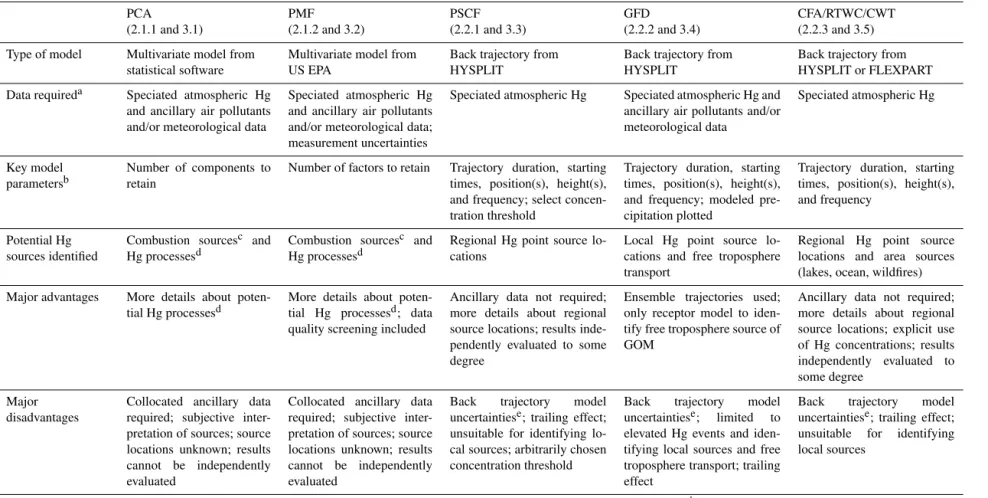
Table 1.Summary of receptor models used in speciated atmospheric mercury studies (see relevant sections in parentheses).
PCA (2.1.1 and 3.1)
PMF (2.1.2 and 3.2)
PSCF (2.2.1 and 3.3)
GFD (2.2.2 and 3.4)
CFA/RTWC/CWT (2.2.3 and 3.5)
Type of model Multivariate model from statistical software
Multivariate model from US EPA
Back trajectory from HYSPLIT
Back trajectory from HYSPLIT
Back trajectory from HYSPLIT or FLEXPART
Data requireda Speciated atmospheric Hg and ancillary air pollutants and/or meteorological data
Speciated atmospheric Hg and ancillary air pollutants and/or meteorological data; measurement uncertainties
Speciated atmospheric Hg Speciated atmospheric Hg and ancillary air pollutants and/or meteorological data
Speciated atmospheric Hg
Key model parametersb
Number of components to retain
Number of factors to retain Trajectory duration, starting times, position(s), height(s), and frequency; select concen-tration threshold
Trajectory duration, starting times, position(s), height(s), and frequency; modeled pre-cipitation plotted
Trajectory duration, starting times, position(s), height(s), and frequency
Potential Hg sources identified
Combustion sourcesc and Hg processesd
Combustion sourcesc and Hg processesd
Regional Hg point source lo-cations
Local Hg point source lo-cations and free troposphere transport
Regional Hg point source locations and area sources (lakes, ocean, wildfires)
Major advantages More details about poten-tial Hg processesd
More details about poten-tial Hg processesd; data quality screening included
Ancillary data not required; more details about regional source locations; results inde-pendently evaluated to some degree
Ensemble trajectories used; only receptor model to iden-tify free troposphere source of GOM
Ancillary data not required; more details about regional source locations; explicit use of Hg concentrations; results independently evaluated to some degree
Major disadvantages
Collocated ancillary data required; subjective inter-pretation of sources; source locations unknown; results cannot be independently evaluated
Collocated ancillary data required; subjective inter-pretation of sources; source locations unknown; results cannot be independently evaluated
Back trajectory model uncertaintiese; trailing effect; unsuitable for identifying lo-cal sources; arbitrarily chosen concentration threshold
Back trajectory model uncertaintiese; limited to elevated Hg events and iden-tifying local sources and free troposphere transport; trailing effect
Back trajectory model uncertaintiese; trailing effect; unsuitable for identifying local sources
aSource emissions profiles are necessary to interpret PCA and PMF results; Hg emissions data from inventories or models are required to evaluate back trajectory results.bRefer to specific models for details on all model inputs and
parameters.cCombustion sources include coal combustion, biomass burning, and vehicular, industrial and waste incineration emissions.dHg processes include meteorological influence on seasonal and diel patterns, GEM oxidation, Hg
emissions from the ocean and snowmelt, and GOM and PBM wet deposition, which may impact speciated atmospheric Hg at the receptor location.eBack trajectory uncertainties include distance traveled by single trajectories or excluding Hg transformation and deposition processes
www
.atmos-chem-ph
ys.net/15/7877/2015/
Atmos.
Chem.
Ph
ys.,
15,
7877–
7895
,
light potential sources areas affecting the receptor measure-ments. Areas with high PSCF values (approaching 1) have a higher probability of airflows contributing to elevated atmo-spheric Hg concentrations at the receptor site.
PSCFij = mij
nij
Wij (4)
The mean atmospheric Hg concentration over the entire sam-pling period and/or particular season is the threshold selected formij in many PSCF studies for speciated atmospheric Hg (Han et al., 2005, 2007; Choi et al., 2008; Xu and Akhtar, 2010; Fu et al., 2011, 2012a, b). Other studies have used the 75th percentile concentration as the concentration threshold (Lee et al., 2014) or determined a suitable threshold from short-term elevated GEM events (Abbott et al., 2008). A map of the model domain is typically divided into grid cell sizes of 1◦×1◦(Han et al., 2005; Choi et al., 2008; Xu and Akhtar, 2010); however, a finer grid has also been applied, e.g., 0.5◦
×0.5◦, 0.25◦×0.25◦, or 0.2◦×0.3◦(Abbott et al.,
2008; Fu et al., 2011, 2012a, b; Lee et al., 2014). In general, the size of the grid cells depend on the study area considered (Hopke, 2003).
To determine PSCF, a large number of back trajectories were generated using the HYSPLIT model. PSCF studies of speciated atmospheric Hg used archived meteorological data sets available in the HYSPLIT model, such as EDAS (Eta Data Assimilation System) for North American loca-tions (Han et al., 2005, 2007; Abbott et al., 2008; Choi et al., 2008; Xu and Akhtar, 2010) and GDAS (Global Data As-similation System) for sites in China (Fu et al., 2011, 2012a, b) and Korea (Lee et al., 2014). The back trajectory duration selected in most PSCF studies ranged from 72 to 120 h for GEM and TGM (Choi et al., 2008; Xu and Akhtar, 2010; Fu et al., 2012a, b), whereas Abbott et al. (2008) generated 24 h trajectories. A 48 h trajectory duration was typically chosen for GOM and PBM (Han et al., 2005; Choi et al., 2008) be-cause of their shorter atmospheric residence time compared to GEM. Since the daily mean speciated atmospheric Hg con-centration was used to determine PSCF values, trajectories were generated at intervals of 24 h (Xu and Akhtar, 2010; Fu et al., 2012a) or 6 h (Han et al., 2005, 2007) to represent the airflows for a sampling day. For 7.5 h GOM and 3.5 h PBM samples, Fu et al. (2012a) generated back trajectories at inter-vals of 8 and 4 h, respectively. Most studies computed back trajectories at a single start height representative of the mix-ing height of the boundary layer, such as 100 or 500 m above model ground level, whereas Fu et al. (2011, 2012a, b) de-termined back trajectories at multiple starting heights (e.g., 500, 1000, 1500 m).
After determining the number of trajectory segment end-points in each grid cell, a weighting factor was typically ap-plied to PSCF values in some studies if the number of the endpoints in a grid cell was less than 2 or 3 times the av-erage number of endpoints in all the grid cells (Han et al., 2005, 2007; Xu and Akhtar, 2010; Fu et al., 2011, 2012a, b;
Lee et al., 2014). In one study, grid cells with less than four trajectory segment endpoints were omitted from the PSCF calculation (Abbott et al., 2008).
The advantage of PSCF over the multivariate receptor models is that it provides the spatial distribution of poten-tial source areas contributing to the receptor site. With PSCF, regional anthropogenic point sources can be identified if the locations of Hg point sources are plotted together with the PSCF results. In contrast, multivariate models infer poten-tial types of sources but do not provide information about where the Hg sources are located. PSCF also does not re-quire ancillary pollutant measurements. This data may not be available at the receptor location, and the sampling reso-lution may not be the same as the speciated atmospheric Hg data, which require additional data processing. The disadvan-tages with PSCF are related to back trajectory modeling of speciated atmospheric Hg since the models may not simu-late chemical reactions, gas-particle partitioning processes, and Hg deposition. There are also uncertainties with the dis-tance traveled by single back trajectories (Stohl, 1998; Wat-son et al., 2008). Due to the back trajectory model resolution, PSCF is not ideal for identifying potential local sources. In addition to disadvantages of trajectory models, the majority of the trajectory segment endpoints are found near the recep-tor location where all the back trajecrecep-tories converge (Watson et al., 2008). The largernij affects the PSCF calculation in Eq. (4) because it results in a larger denominator and may lead to a lower PSCF value. This also depends on the concen-tration threshold selected because a smaller threshold likely produces higher PSCF values.
2.2.2 Gridded frequency distributions (GFD) description
I. Cheng et al.: Overview of receptor-based mercury source apportionment studies 7883 GFD has only been applied to data subsets, such as
el-evated or enhanced speciated atmospheric Hg events. In Weiss-Penzias et al. (2009), the enhancement event was de-fined by the simultaneous occurrence of GOM concentra-tions at>75th percentile of the daily mean at three nearby receptor locations. In another study, GFD was determined for GOM enhancement events in which at least one con-centration exceeded the 98th percentile (Weiss-Penzias et al., 2011). The length of a GOM enhancement event was deter-mined by measurements above the mean concentration. The events were further stratified into data subsets impacted by local sources and free troposphere transport. The first data subset was derived by analyzing the frequency distributions of GOM/SO2ratios. The second data subset had GOM con-centrations similar to the first data subset, but SO2 concen-trations were much lower (Weiss-Penzias et al., 2011). A similar approach for defining GOM enhancement events was also adopted by Gustin et al. (2012). The data subset used to generate the GFD was limited to a specific range of wind directions in order to verify the sources of GOM enhance-ment events were due to several local electricity power plants (Gustin et al., 2012).
The advantage of GFD over other back trajectory recep-tor models is the generation of trajecrecep-tories at multiple start-ing locations and heights. Ensemble trajectories illustrate the variability in the pollutant transport pathways, which indi-cates how uncertain a single trajectory can be (Stohl, 1998; Hegarty et al., 2009; Gustin et al., 2012). Some of the disad-vantages of PSCF also apply to GFD, such as back trajectory uncertainties and higher number of trajectory endpoints ap-proaching the receptor location discussed in Sect. 2.2.1. The GFD model was applied to only small data subsets that met a specific criteria and therefore excluded a large proportion of the entire data set. Classification of the data subsets also re-quires knowledge about the sources contributing to elevated pollutant concentrations at the receptor site.
2.2.3 Concentration field analysis (CFA), residence time weighted concentration (RTWC), concentration-weighted trajectory (CWT) description
CFA, RTWC, and CWT are also common back trajectory receptor models that have been used to identify potential source areas contributing to speciated atmospheric Hg mea-surements (Han et al., 2007; Rutter et al., 2009; de Foy et al., 2012; Cheng et al., 2013b). The most apparent difference be-tween CFA/RTWC/CWT and previously described back tra-jectory receptor models is that the tratra-jectory residence time in the grid cells have been weighted by the observed at-mospheric Hg concentrations corresponding to the arrival of each trajectory. CFA, RTWC, and CWT can be summarized by Eq. (5) (Kabashnikov et al., 2011):
Pij= L P l=1
clτij l
L P l=1
τij l
. (5)
Pij represents the source intensity of a grid cell (i, j ) con-tributing to the receptor location.cl is the speciated atmo-spheric Hg concentration corresponding to the arrival of back trajectorylin the CWT model. For CFA or RTWC, logarith-mic concentrations are used.τij l is the number of trajectory segment endpoints in grid cell (i, j )for back trajectoryl
di-vided by the total number of trajectory segment endpoints for back trajectoryl (i.e., residence time of a trajectory in each
grid cell);Lis the total number of back trajectories over a time period (e.g., entire sampling period or a season) (Cheng et al., 2013b). As the model equation shows, higher atmo-spheric Hg concentrations would lead to higher source inten-sity if the trajectory residence time were the same. In CFA, RTWC, and CWT, the trajectory residence time scaled by the observed concentration is also normalized by the trajectory residence time.
The FLEXPART-WRF (FLEXible PARTicle-Weather Re-search and Forecasting) model simulates the transport and dispersion of air pollutants (Stohl et al., 2005; Fast and Easter, 2006). In CFA studies for speciated atmospheric Hg, FLEXPART-WRF simulated the path of 100–1000 particles released from the receptor location (Rutter et al., 2009; de Foy et al., 2012). The particles were tracked for 48 h in Rutter et al. (2009), since CFA was applied to speciated atmospheric Hg data. Six-day trajectories were determined by de Foy et al. (2012) to simulate the transport of GEM. The hourly lo-cations of the particles are counted in all the grid cells that have been overlaid on a map of the study area. The HYS-PLIT back trajectory model using the EDAS 40 km archived meteorological data was used in the CWT studies for spe-ciated atmospheric Hg (Cheng et al., 2013b). Back trajecto-ries of 48 h were generated for each 3 h GEM, GOM, and PBM concentration at a single start height representative of the coastal location. The hourly locations or trajectory seg-ment endpoints for every trajectory are tallied for all grid cells. CWT was determined for grid cells with at least two sets ofclandτij l.
As summarized in Table 1, the advantage of CFA and CWT over PSCF and GFD described in previous sections is the integration of the receptor concentrations in the back tra-jectory model as evident in Eq. (5). This is important because the observed concentrations account for the various physical and chemical processes as an air pollutant is transported from sources to the receptor site (Jeong et al., 2011). PSCF uses a concentration threshold to determine the trajectory residence time associated with elevated Hg concentrations; however, it may be perceived as arbitrary. Consequently, the recep-tor measurements that are slightly below the threshold
centration are excluded from PSCF calculation (Han et al., 2007). Another advantage of CFA and CWT is that the source intensity of the grid cells is normalized by the trajectory res-idence time, which reduces the bias due to increasing trajec-tory residence time near the receptor location. In the CFA studies for speciated atmospheric Hg, the use of a particle dispersion trajectory model is more suitable for simulating turbulent flows and has been validated by tracer experiments (Hegarty et al., 2013). The disadvantages of CFA and CWT are the uncertainties associated with back trajectory model-ing, especially when single trajectories are generated (Stohl, 1998). Common to many of the back trajectory receptor mod-els described in this section and previously, the potential Hg source areas identified by the models are not often evaluated against Hg emissions inventory quantitatively, which makes it difficult to determine the accuracy of the models at recon-structing the sources (Kabashnikov et al., 2011). This evalu-ation requires a comprehensive Hg emissions inventory be-cause both anthropogenic and natural sources contribute sig-nificantly to global Hg emissions (Pirrone et al., 2010).
3 Overview of existing studies 3.1 PCA results
3.1.1 Source apportionment
PCA has been used to apportion potential sources affecting TGM and speciated atmospheric Hg in Seoul, South Korea (Kim and Kim, 2001; Kim et al., 2011); Changbai Moun-tain (Wan et al., 2009a, b) and Xiamen (Xu et al., 2015), China; Göteberg, Sweden (Li et al., 2008); Poland (Majew-ski et al., 2013); Canada; and the US. The Canadian sites are located in Point Petre and Egbert, Ontario (Blanchard et al., 2002); CAMNet stations (Temme et al., 2007), Toronto (Cheng et al., 2009), northwestern Ontario (Cheng et al., 2012); Kejimkujik National Park (Cheng et al., 2013a); Flin Flon, Manitoba (Eckley et al., 2013); Fort McMurray, Al-berta (Parsons et al., 2013); and Windsor, Ontario (Xu et al., 2014). The US sites included south Florida (Graney et al., 2004); Detroit, Michigan (Lynam and Keeler, 2006; Liu et al., 2007); Mount Bachelor, Oregon (Swartzendruber et al., 2006); Athens, Ohio (Gao, 2007); Rochester, New York (Huang et al., 2010); and Grand Bay, Mississippi (Ren et al., 2014). Most of the studies identified a factor/component that was representative of combustion sources (e.g., coal com-bustion, vehicular, industrial, biomass burning, and waste in-cineration emissions) regardless of whether the studies were conducted in urban, rural, or coastal locations. This com-ponent generally consisted of high comcom-ponent loadings on Hg and other air pollutant markers, such as NOx, SO2, O3, PM2.5, black carbon, CO, and/or trace metals. A component consisting of GEM, NOx, and CO was attributed to vehicu-lar emissions in Detroit (Lynam and Keeler, 2006). Graney
et al. (2004) was able to narrow down the PBM source in south Florida to waste incineration because of the presence of PBM, V and Ni in one of the components. Higher load-ings for TGM, Ag, Cd, Cr, Mn, Mo, Se, Sn and Zn at a ru-ral location in Point Petre were assigned to distant anthro-pogenic/coal combustion sources (Blanchard et al., 2002). The presence of NOx, SO2and PM2.5 in a component was assigned to marine transportation after verifying that the back trajectories passed over shipping ports along the US east coast (Cheng et al., 2013a). The percent variance that can be explained by anthropogenic combustion sources varied from 10 to 57 % among the studies reviewed. It explained most of the variance (>35 %) at some urban locations, such
as in Seoul, Toronto, Windsor, and south Florida because of the proximity to Hg point sources and/or traffic (Kim and Kim, 2001; Graney et al., 2004; Cheng et al., 2009; Xu et al., 2014). At rural locations further away from Hg point sources and traffic, 15–29 % of the variance was explained by the transport of anthropogenic combustion emissions (Blanchard et al., 2002; Cheng et al., 2012, 2013a). The PCA studies of atmospheric Hg also attributed the sources of TGM and PBM at rural sites to crustal sources (Blanchard et al., 2002; Graney et al., 2004; Cheng et al., 2012, 2013a). This compo-nent typically included TGM or PBM and Si, Al, Fe, Mn, Sr, Ti, Ca2+, Mg2+, and/or K+and explained between 12 and 41 % of the variance in the data set.
I. Cheng et al.: Overview of receptor-based mercury source apportionment studies 7885 GEM oxidation was a larger contributor to the receptor
measurements (31 % of the total variance) than combustion sources during July in Detroit. This component included strong positive component loadings on GOM, O3, tempera-ture and wind speed, and negative loadings on relative hu-midity (Lynam and Keeler, 2006). Other studies also ex-tracted a component representative of GEM oxidation with similar pollutant or meteorological parameter loadings; how-ever, the component did not explain the most variance with percentages ranging from 11 to 27 % (Li et al., 2008; Huang et al., 2010; Cheng et al., 2012, 2013a; Ren et al., 2014; Xu et al., 2014). GEM oxidation was also inferred from a PCA component containing GOM, BrO and O3(Ren et al., 2014). Although BrO and O3are potential oxidants of GEM, it is unclear from this component whether the oxidation reaction was dominated by BrO or O3and occurring in the gas, liq-uid, and/or solid phase. This example shows that inferring the GEM oxidation contribution from PCA results is compli-cated by Hg chemistry uncertainties. This component could also be interpreted as a combined effect from several oxi-dants or the co-occurrence of O3, BrO and GOM photochem-ical reactions because the strong loadings on the parameters is due to their strong correlations and not necessarily reflec-tive of any causal relationships.
Diurnal mixing was also identified as the primary com-ponent affecting GEM concentrations in Detroit (Liu et al., 2007). The component explained 27 % of the variance in the data set and was composed of negative component loadings for GEM, PBM and other primary pollutant variables (SO2 and NOx), and positive loadings for O3. It is consistent with daytime mixing between the surface air and cleaner air aloft, which likely resulted in the lower GEM and PBM concentra-tions in the afternoon. Photochemical production of O3also occurs during daytime. Liu et al. (2007) also confirmed that the principal component scores were higher for daytime data than nighttime, indicating that this component contributed more to daytime measurements. In contrast to diurnal mix-ing, another study obtained strong component loadings on GEM and other primary air pollutants for the nighttime data subset, which was largely attributed (40.3 % of the total vari-ance) to nocturnal atmospheric inversion in Göteberg, Swe-den (Li et al., 2008). During nighttime atmospheric inversion, air near the surface is colder and denser than the air above it, which leads to reduced mixing and inhibits air pollutant dis-persion.
Snowmelt and evasion from the ocean are two processes that were identified from PCA as potential sources of GEM. Snowmelt was inferred from PCA of the winter data sub-sets from Rochester, New York (Huang et al., 2010), and explained the most variance in the winter data (19–21 %). The study obtained positive component loadings on GEM, temperature, and a “melting” variable, which is coded based on temperature ranges above 0◦C. Additional analysis also confirmed that the average GEM concentrations correspond-ing to temperatures above 0◦C were statistically higher
than those below 0◦C. Instead of snow melting, Eckley et al. (2013) collected snow depth data and obtained a neg-ative loading for the component assigned to surface GEM emission. Evasion of GEM from the Atlantic Ocean was recognized as a potential source of GEM to a coastal site in Atlantic Canada (Cheng et al., 2013a). PCA produced a component with high loadings on GEM, relative humidity, wind speed, and precipitation, which explained 12–25 % of the variance in the data set. Further analysis using absolute principal component scores and back trajectory data indi-cated that this component impacted sampling days that were influenced by marine airflows. Back trajectories originating from the Atlantic Ocean were also associated with higher rel-ative humidity and wind speed, which is consistent with the component loadings. The meteorological variables present in both of these components are also consistent with those ob-served in field studies (Lalonde et al., 2003; Laurier et al., 2003).
A component representing PBM wet deposition was also extracted from data sets collected in Rochester (Huang et al., 2010) and Huntington Wildlife Forest (Cheng et al., 2013a), New York. Hg wet deposition was inferred from the presence of high negative loadings for PBM and positive loadings for precipitation and relative humidity. Huang et al. (2010) also reported negative loadings on barometric pressure, since low atmospheric pressure leads to precipitation. Hg wet deposi-tion explained 12–14 % of the variance in the seasonal data subset (Huang et al., 2010) and 8 % of the variance in an an-nual data set (Cheng et al., 2013a).
3.1.2 Site characteristics on PCA results
Some unique factors have been identified owing to site char-acteristics, such as a high altitude location, urban site, and forested area. A component consisting of GOM, O3, and wa-ter vapor was the primary component extracted from a data set (47 % of the total variance) collected at a high altitude site in the Mount Bachelor Observatory in Oregon, US. It was in-terpreted as transport from the free troposphere because of a positive component loading on O3and a negative component on water vapor (i.e., dry air) which are characteristics of the upper atmosphere (Swartzendruber et al., 2006). Unlike other studies, the presence of O3was not indicative of its role as a potential oxidant of GEM. This elevated site (2.7 km above sea level) was frequently impacted by the free troposphere because of the diurnal cycle of mountain winds and off-shore winds from the Pacific Ocean (Swartzendruber, 2006). Mountain winds move upslope during daytime. At night, free troposphere transport is driven by downslope winds. The in-fluence of the free troposphere has been verified by perform-ing additional back trajectory analysis (see Sect. 3.4). Dry upper troposphere air also impacted other high elevation sites (Faïn et al., 2009; Timonen et al., 2013). Faïn et al. (2009) observed an anti-correlation between GOM and GEM dur-ing low relative humidity conditions, while GOM was not
lated to other air pollutants or O3. Timonen et al. (2013) sug-gested that GEM oxidation by O3and halogens and hetero-geneous chemistry may occur during long-range transport of air masses from Asia. GEM oxidation by halogens can also occur in clean air masses originating from the Pacific Ocean. These findings are consistent with the rapid GEM oxidation by bromine occurring in the free troposphere simulated in at-mospheric Hg models (Holmes et al., 2006). However, there is still ongoing debate on which atmospheric oxidants are in-volved in GEM oxidation.
In urban sites, GEM oxidation and industrial sulfur are the top two components. Transport was the most frequent component in rural settings. Huang et al. (2010) suggested that the aqueous-phase reaction of GEM with O3in some re-gions may be the most important oxidation process. Huang et al. (2010), Akhtar (2008), and Lynam and Keeler (2006) de-termined industrial sulfur was a major factor affecting mer-cury. The study by Lynam and Keeler (2006) was located in Detroit, Michigan, which was close to industrial areas. Akhtar (2008)’s study was conducted in Windsor, Ontario, Canada, downwind of several industrial states in the US, in-cluding Michigan, Ohio, and Indiana. The study of Huang et al. (2010) was carried out in Rochester, downwind of large coal-fired power plants located in western New York.
Forest fire smoke was inferred from PCA results which had positive loadings on TGM and the components of for-est fire smoke, namely PM2.5, CO, and NH3(Parsons et al., 2013). This study was conducted in Alberta, Canada, where the forest density and occurrence of forest fires are both high. TGM/CO emissions ratios have also been used to
differenti-ate the impact of biomass burning from anthropogenic emis-sions on receptor measurements. Based on aircraft and high altitude measurements, the median TGM/CO ratio can range from 1.3 to 9.2 pg m−3ppb−1 among different regions. A low TGM / CO ratio (1–2 pg m−3ppb−1)is clearly attributed to biomass burning plumes, whereas a higher TGM/CO ratio (>6 pg m−3ppb−1) is strongly indicative of anthro-pogenic emissions (Ebinghaus et al., 2007; Weiss-Penzias et al., 2007; Slemr et al., 2014). The TGM/CO ratio could be used in PCA for this purpose when a component contains only TGM and CO and no other chemical species markers are available. A potential method could be to calculate the absolute principal components scores (APCS) and convert it to a pollutant’s source mass contribution to the receptor mea-surements (Thurston and Spengler, 1985). The TGM/CO
ratio calculated from TGM and CO’s source mass contribu-tions are then compared with the emission ratios for biomass burning and anthropogenic plumes. The APCS method may be extended to TGM/CO2 and TGM/CH4 ratios to gain insight into where the plumes originated from by comparing the ratios to those in literature (e.g., Slemr et al., 2014). Aside from forest fires, road-salt particles were identified as a po-tential PBM source at another forested site because of the existence of PBM, Na+, and Cl−. The authors pointed out that the most probable source of PBM during winter is the
road dust which contains road salt and PBM via absorption or condensation of gaseous Hg (Cheng et al., 2012, 2013a).
3.1.3 PCA results from data subsets
To investigate different effects of Hg sources or atmospheric processes on annual, seasonal or diurnal scales, some stud-ies divided the full data set into subsets for additional PCA investigations. All papers reported differences between the subsets and between the full data set and the subsets to some extent (Gao, 2007; Parsons et al., 2013, Xu et al., 2014). In the 2007–2011 Windsor, Ontario, TGM study (Xu et al., 2014), seasonal PCA revealed that the transport component seems to be very influential to TGM concentrations due to high winds. The impact of GEM oxidation was more eas-ily extracted from the springtime data because there are less confounding factors, e.g., re-emission of GEM. When ana-lyzed by year, similar results were obtained as with the full data set. In a study conducted in Ohio, two factors (coal-fired power plants and GEM oxidation) were extracted from the full data set. The PCA result from summer subset was sim-ilar, component one being coal-fired power plants and GEM oxidation, and component two being combustion. The winter subset also had two factors retained: combustion and coal-fired power plants, however, without GEM oxidation (Gao, 2007).
Similarly, TGM data collected in Fort McMurray, Alberta, were stratified into three concentration ranges and then each data subset were analyzed separately using PCA (Parsons et al., 2013). For the full data set, TGM variability was pri-marily attributed to diurnal variability followed by forest fire smoke, temperature and snow depth, industrial sulfur, and combustion processes. However, when the highest one-third TGM concentration subset was analyzed, the two major Hg components extracted were forest fire smoke and diur-nal variability. This suggests that elevated TGM concentra-tions were not strongly attributed to oil sand activities. The middle one-third and lowest one-third TGM concentration ranges show the same result as the full data set with diurnal variability as the major Hg component.
I. Cheng et al.: Overview of receptor-based mercury source apportionment studies 7887 Liu et al. (2007), who reported that PBM has a similar
di-urnal pattern as GOM. Specifically, GOM generally peak from midday to afternoon, and is quickly removed by night-time dry deposition. A comparison of TGM and speciated Hg PCA results was also examined by Wan et al. (2009a, b). The same data set was analyzed twice. The initial analy-sis with TGM only resulted in meteorological conditions as the major Hg component (Wan et al., 2009a). When all three Hg species were included, diurnal trend and combustion pro-cesses were identified as the major Hg components (Wan et al., 2009b).
Of all Hg components reported in 10 speciated Hg stud-ies, one-half of the components involved GOM while only 10 % of the components contained all three Hg species. PBM tended to cluster on a component with GEM or GOM rather than on a separate factor, indicating that these species may undergo gas-particle partitioning (Lynam and Keeler, 2006). None of the components had GEM and GOM clustered to-gether, suggesting differences in the strength of sources and sinks for GEM and GOM.
3.1.5 PCA results summary
Due to the inherent difficulties in component interpretation, some PCA studies were not able to characterize certain com-ponents due to a lack of data/evidence. For example, Cheng et al. (2009) derived a major Hg component with high load-ings for all three Hg species and PM2.5 only, which could not be easily characterized without additional data. Wan et al. (2009b) were unable to differentiate two of the compo-nents, which were only labeled “Combustion processes I” and “Combustion processes II”. Most PCA studies have gone beyond apportioning conventional anthropogenic sources to even identifying chemical and physical processes (e.g., GEM oxidation, boundary layer mixing, and surface GEM flux). The inclusion of meteorological parameters has helped with the interpretation of Hg processes. However, the profiles for these Hg processes and some non-point sources are not well-established. The qualitative interpretation of the components is based on literature. A few PCA studies included other re-ceptor model (e.g., back trajectory models and absolute prin-cipal component scores) results to support the PCA findings. PCA results were often verified by performing analysis of seasonal and diel trends in atmospheric Hg, correlations be-tween Hg and ancillary air pollutants, and wind speeds and wind directions. Despite the supplementary data analysis, PCA results for speciated atmospheric Hg are rarely evalu-ated. Only a few studies have compared PCA output to other data reduction or data classification outputs, such as a pos-itive matrix factorization (PMF) model and cluster analysis (Cheng et al., 2009, 2012).
3.2 PMF Results
The PMF model apportioned sources of speciated atmo-spheric Hg measured in Potsdam (Liu et al., 2003) and Rochester (Wang et al., 2013), New York, and Toronto, Canada (Cheng et al., 2009). PMF inferred industrial sources, such as nickel smelting and metal production, as potential contributors to atmospheric Hg in Potsdam, New York, and Toronto, Canada. Among the seven factors extracted from the Potsdam site, GEM was found in trace concentrations in one factor containing Se and S, which are characteristic of nickel smelting. This source was also verified by PSCF, which indicated that the probable source areas were nickel smelting operations in central Quebec and eastern Ontario (Liu et al., 2003). Metal production was also identified as a potential source contributing to GOM and PBM concentra-tions in Toronto based on comparison of the pollutant ratios (e.g., NO2/TGM, PM2.5/TGM, and SO2/TGM) between factor profiles and source profiles from emissions inventories (Cheng et al., 2009). However, due to the large variability in the source emissions ratios among metal production plants, several factor profiles were assigned to production of met-als. The source with the most unique and least variability in the source emissions ratios was sewage treatment; thus, one of the factors was easily interpreted as sewage treatment. Of all GEM concentrations, 84 % were attributed to this source. This study highlighted the potential issues with multivariate models, such as non-unique factor profiles, that can arise due to a lack of chemical species markers in the data set. If trace metals or aerosol chemical composition data were available at this receptor location, Zn, Pb, Cu, Cl, V, and Ni could be used as chemical species markers for municipal waste dis-posal/incineration (Graney et al., 2004; Keeler et al., 2006; Watson et al., 2008). In the absence of this data, potential Hg sources in urban areas may have been neglected, such as GEM emissions from urban surfaces and soil (Eckley and Branfireun, 2008) and vehicular traffic (Landis et al., 2007).
Inclusion of CO and aerosol measurements in Rochester was practical for assigning factors from the PMF model to traffic and wood combustion sources and the process of nucleation. Out of these three factors, however, only wood combustion contributed significantly to PBM concentrations (48 %) as well as to ultrafine and fine particle number con-centrations and Delta-C. PBM contribution from wood com-bustion was comparable to that from a local coal-fired power plant (CFPP) in Rochester. The source with the largest con-tribution to GEM concentrations was a factor with enhanced ozone contributions (50 %). Factors representing CFPP and GEM oxidation contributed 50 and 85 %, respectively, to GOM concentrations (Wang et al., 2013). The PMF model was also applied to the data set collected before and after the shutdown of the CFPP to show the change in the impact of this source on speciated atmospheric Hg in Rochester. CFPP contribution declined by 25 % for GEM, 74 % for GOM, and 67 % for PBM after the CFPP was shutdown. These results
were also verified by condition probability function, which showed a substantial decrease in the probability of observing elevated concentrations from the wind direction of the CFPP after its closure (Wang et al., 2013).
There were only a few studies that have used the PMF model to apportion sources of speciated atmospheric Hg. The studies identified local and regional sources and chem-ical and physchem-ical processes impacted speciated atmospheric Hg. The PMF model was also capable of investigating the change in source emissions on speciated atmospheric Hg at a receptor site. Having a sufficient number of chemical species markers in the data set is conducive to the interpretation of the model factors and also ensures that some sources have not been omitted. To verify the anthropogenic point sources re-solved from the PMF model, studies performed further anal-ysis using PSCF and conditional probability function. Un-like the PCA studies, some discussion was provided on the goodness of fit of the PMF model. However, the sources in-ferred have not been independently assessed for accuracy in PMF studies of speciated atmospheric Hg. In comparison, source-based Hg transport models can evaluate the predicted speciated atmospheric Hg concentrations against field mea-surements.
3.3 PSCF results
PSCF was applied to receptor locations in North America and Asia, such as Potsdam, Stockton, Sterling (Han et al., 2005, 2007) and Huntington Wildlife Forest (Choi et al., 2008), New York; Salmon Falls Creek, Idaho (Abbott et al., 2008); Windsor, Ontario, Canada (Xu and Akhtar, 2010); Guiyang, Waliguan, and Mt. Changbai, China (Fu et al., 2011, 2012a, b); and Yeongheung Island, South Korea (Lee et al., 2014). Most of the studies used PSCF to analyze TGM or GEM data, with the exception of two studies that analyzed speciated atmospheric Hg as well (Han et al., 2005; Choi et al., 2008).
Four of the PSCF studies were conducted in the Great Lakes region close to Lake Erie and Lake Ontario. These studies identified potential source areas to the south of the receptor site spanning from the Ohio River valley, which is known for its industrialized areas, to Texas. From these potential source areas, the studies located Hg point sources from emissions inventory, such as coal combustion in Ohio and Pennsylvania, waste incineration and oil combustion in St. Louis, and metal smelting in Ontario and Quebec. The Atlantic Ocean and Gulf of Mexico were also recognized as potential sources of GEM and TGM through potential photo-reduction of Hg(II) in the ocean and volatilization of GEM from the ocean surface (Han et al., 2007; Xu and Akhtar, 2010). In a western US site, GEM was attributed to Hg point sources, gold mining, natural Hg-enriched areas in Nevada, and wildfires (Abbott et al., 2008). At receptor locations in China, PSCF identified potential source regions of TGM and GEM in north-central China, northwestern India, and North
Korea (Fu et al., 2011, 2012a, b). In these regions, Hg emis-sions originate from coal combustion, cement production, and urban and industrial areas. Mercury emissions in north-eastern China and local industrial emissions also contributed to elevated TGM in South Korea (Lee et al., 2014).
Seasonal PSCF analysis revealed potential source areas that were not recognized in PSCF analysis of long-term data. The change in the prevailing winds in Guiyang, China, dur-ing the summer was driven by monsoons, which led to the identification of potential source areas southeast of Guiyang (Fu et al., 2011). In Windsor, Canada (Great Lakes region), PSCF analysis of the winter and spring TGM data revealed potential source areas in the northwest and northeast direc-tions, whereas the source areas based on the PSCF analysis of the annual data were predominantly transboundary pollution from the US (Xu and Akhtar, 2010). Xu and Akhtar (2010) attributed this finding to the use of seasonal means to per-form seasonal PSCF analysis because more sampling days were above the seasonal mean concentration threshold than the annual mean.
PSCF results were correlated with Hg point source emis-sions data in a few PSCF studies (Han et al., 2005, 2007; Choi et al., 2008). Correlation coefficients ranged from 0.34 to 0.55 and appeared to be dependent on trajectory model parameters and Hg emissions data used. Han et al. (2005) obtained stronger correlations for a trajectory model, which simulated dispersion, than those of a single trajectory model and a trajectory model simulating both dispersion and de-position. The duration of the trajectory for simulating GEM transport also affected the correlation results. When longer trajectories (i.e., 5-day) were used in PSCF and were cor-related with total Hg emissions (sum of GEM, GOM and PBM), correlation coefficients were higher than PSCF anal-ysis using 3-day trajectories (Han et al., 2007). On the contrary, shorter trajectories used in PSCF produced better agreement with the emissions inventory for GEM only. In the GOM source–receptor relationship study, Han et al. (2005) compared PSCF results to the GOM emissions inventory but noted that the uncertainties in the GOM emissions inventory are likely larger than those of GEM. The studies attributed the weak to moderate correlations between PSCF results and Hg point source emissions to emissions database uncertain-ties, such as the use of emission factors instead of measure-ments to determine Hg emissions, and an incomplete Hg emissions inventory.
I. Cheng et al.: Overview of receptor-based mercury source apportionment studies 7889 RTWC prevented the identification of potential source
ar-eas downwind and upwind of actual point sources, which is known as the trailing effect. The trailing effect also led to the overestimation of the impact of regional source ar-eas on GEM concentrations in Guiyang, China, because of significant local Hg sources along the same direction (Fu et al., 2011). Additional analysis of wind speeds measured in Guiyang was performed to assess the impact of local sources. The impact of local urban areas on TGM in Mt. Changbai, China, was not identified by PSCF because the model reso-lution of the back trajectories was not suitable for simulating local winds (Fu et al., 2012b). Potential mixing between re-gional airflows and local winds is also a major uncertainty of the PSCF model (Xu and Akhtar, 2010).
PSCF studies on speciated atmospheric Hg identified the regional transport of emissions from Hg point sources, ur-ban areas, and from the ocean. The studies typically reported potential source areas covering a large geographical area be-cause the size of the model grid cells used in the studies is too coarse to accurately locate the point sources. In con-trast to the multivariate models, the PSCF studies rarely dis-cussed potential Hg emissions from forest fires, wood com-bustion, GEM oxidation, crust and soil, and snow melting in the high probability source regions. The PSCF model can be independently evaluated to some degree using Hg emissions data unlike the multivariate models; however, this has only been performed in a few PSCF studies. Based on the lim-ited evaluation of PSCF, trajectory parameters, trailing effect, and Hg emissions data remain to be the major PSCF uncer-tainties and limitations. Therefore, PSCF is more suitable for receptor locations that are potentially impacted by regional or long-range sources rather than locations that are down-wind of major local sources. If only PBM are measured, these models would be more suitable for receptor locations that are potentially impacted by regional sources and less suitable for identifying distant sources because of the shorter residence time of aerosols.
3.4 GFD results
GFD analyses on the horizontal and vertical distribution of trajectory endpoints corresponding to GOM enhance-ment events were conducted in desert valley sites in Nevada (Weiss-Penzias et al., 2009) and coastal sites in the US south-east (Weiss-Penzias et al., 2011; Gustin et al., 2012). The GFD plots for the Nevada sites showed a larger number of trajectory endpoints above the model boundary layer for ele-vated GOM concentrations (i.e., upper quartile GOM) than lower quartile GOM concentrations (Weiss-Penzias et al., 2009). Modeled rainfall amounts were also lower for elevated GOM concentrations. These results indicate the Nevada sites were influenced by transport from the free troposphere. Fur-ther analysis of the trajectory residence time within a 3-D source box defined by latitudes<35◦N and altitudes>2 km was also conducted. The study found longer trajectory
res-idence time for the upper quartile GOM than lower quar-tile GOM, which provided additional support for the up-per atmospheric transport hypothesis (Weiss-Penzias et al., 2009). Transport from the upper atmosphere also contributed to some of the GOM enhancement events in the US south-east (Weiss-Penzias et al., 2011). Compared to GOM en-hancement events that were attributed to local coal com-bustion sources, a higher number of grid cells had>75 % of the trajectory endpoints above the model boundary layer for the GOM enhancement events that were impacted by the free troposphere. For these GOM events, the distances cov-ered by the trajectories were longer, which indicated higher wind speeds and long-range transport. A majority of the grid cells also showed less rainfall, which is consistent with the drier air from the free troposphere. Similar GFD results were also obtained at three coastal sites in Florida (Gustin et al., 2012). GOM enhancement events were partially due to lo-cal electricity generating plants and long-range transport as well as transport from the free troposphere. In the latter case, higher GOM concentrations were accompanied by higher mean PBM, which may be consistent with GOM partitioning to aerosols in the upper atmosphere. This theory is supported by speciated atmospheric Hg measurements and modeling in the free troposphere (Murphy et al., 2006; Selin and Jacob, 2008; Holmes et al., 2009; Lyman and Jaffe, 2012).
GFD analysis of trajectory ensemble data has only been applied to elevated GOM events in the western and southeast-ern US. The studies verified the impact of local power plants and found evidence of free troposphere transport of GOM and PBM. Compared to PSCF studies, the GFD results of-fered less insight into regional Hg sources contributing to the receptor sites. Potential reasons could be because Hg sources contribute to the global atmospheric Hg pool rather than spe-cific receptor sites, and it may not be possible to further sep-arate the elevated GOM events by local source and regional source impacts. Consequently, GOM enhancements at the re-ceptor sites were largely explained by local source and free troposphere effects in the GFD studies.
3.5 CFA, RTWC, and CWT results
CFA, RTWC, and CWT have been used to identify potential sources of TGM and speciated atmospheric Hg contributing to multiple sites in New York (Han et al., 2007), Mexico City (Rutter et al., 2009), Milwaukee, Wisconsin (de Foy et al., 2012); and Dartmouth, Nova Scotia (Cheng et al., 2013b). The New York and Milwaukee sites in the Great Lakes re-gion and the Nova Scotia site identified industrial areas in Ohio and the eastern US as potential Hg sources (Han et al., 2007; de Foy et al., 2012; Cheng et al., 2013b). The source areas identified by the RTWC model also revealed that metal industries in Quebec and Ontario, Canada, contributed to TGM in New York (Han et al., 2007). These source ar-eas also affected GOM and PBM concentrations at the Nova Scotia site based on CWT results (Cheng et al., 2013b). Han
et al. (2007) credited the findings to the scaling of trajec-tory residence time using the receptor TGM concentrations, which were relatively higher at one of the sites near Canada. Hg sources in Canada were not identified by PSCF because the trajectory residence times for some grid cells may have been the same for average to high TGM concentrations ac-cording to Eq. (4) (Han et al., 2007). In Milwaukee, the Great Lakes were also recognized by CFA as a potential source of GEM emissions with an estimated flux between 12 000 and 14 000 kg over the 1-year study period (de Foy et al., 2012). Similarly, higher CWT values for GEM in the Atlantic Ocean all year round suggested that the evasion of GEM from the ocean was a potential source of GEM in Nova Scotia (Cheng et al., 2013b). CFA results for the Mexico City sites indicated that the sites were impacted by known Hg point sources, such as cement and chemical production and paper and card-board manufacturing, and by potential unregistered sources and volcanic emissions (Rutter et al., 2009).
The CFA study of the receptor sites in Mexico City iden-tified the same source areas for GEM and GOM and for the urban and rural site. The consistency in the results suggest that the model was capable of identifying the major source areas contributing to speciated atmospheric Hg (Rutter et al., 2009). RTWC and CWT model results were independently evaluated using Hg emissions data from point sources. Han et al. (2007) obtained a correlation coefficient of 0.19 be-tween RTWC values for TGM and total Hg emissions in the model grid cells. In another study, the correlation coef-ficient between CWT values for PBM and total Hg emis-sions in the model grid cells was 0.27, but no relationships were found between CWT values for GEM and GOM and total Hg emissions (Cheng et al., 2013b). In fact, this study found that almost all major source areas of GEM identified by CWT were not associated with any Hg point source emis-sions. Potential explanations for the weak correlation with industrial Hg emissions are the large spatial variability be-tween moderate and strong source regions (Han et al., 2007) and the exclusion of Hg emissions data from non-point Hg sources, such as biomass burning, wildfires, surface mining, and from oceans, lakes, soil, and vegetation (Cheng et al., 2013b). Studies have also discussed potential unregistered Hg sources (Rutter et al., 2009; Cheng et al., 2013b) and the need for additional field measurements to quantify their Hg emissions. Due to the limitations and uncertainties of the Hg emissions database, an alternative approach was used to as-sess the CWT model accuracy by verifying that there were no Hg point source emissions in the weak source regions (Cheng et al., 2013b).
The trailing effect issue was raised in most of the studies. Like PSCF, the CFA, RTWC, and CWT models may not be able to distinguish between upwind and downwind source ar-eas. For example, a single trajectory associated with a very high Hg concentration at a receptor location could overes-timate the impact of distant sources (Rutter et al., 2009; de Foy et al., 2012). A potential solution to the trailing effect
is to redistribute the concentrations along the trajectory seg-ment for every trajectory prior to determining the concentra-tion fields, RTWC, or CWT (Stohl, 1996; Han et al., 2007). de Foy et al. (2012) also suggested using a polar grid, which may increase the overall residence time in the larger distant grid cells. Another way is to assess local source impacts by analyzing local wind patterns, such as conditional probability function (Cheng et al., 2013b). Other sources of uncertainties include variability in the trajectory distance with starting po-sitions for single trajectory applications, Hg deposition, and turbulent mixing (Cheng et al., 2013b).
The CFA, RTWC, and CWT approaches attributed speci-ated atmospheric Hg at receptor locations to regional indus-trial areas with a high density of Hg point sources and Hg emissions from lakes and oceans. The sources identified are similar to PSCF but less comprehensive than the findings of atmospheric chemical and physical processes in the multi-variate receptor modeling studies (see Table 1 summary of the receptor models discussed in this paper). While the ob-jective in most CFA/RTWC/CWT and PSCF studies were to identify potential Hg point sources, these models can also be used at receptor locations that are potentially impacted by area sources (e.g., Hg emissions from lakes, ocean, forest fires, traffic) as shown in de Foy et al. (2012). CFA, RTWC, and CWT results for speciated atmospheric Hg have been independently evaluated to only some extent because of lim-itations and uncertainties of the Hg emissions database and the few model intercomparisons conducted. Similar to PSCF, trajectory model parameters and trailing effect uncertainties also apply to CFA, RTWC, and CWT. Therefore, some of the receptor location considerations for PSCF discussed in Sect. 3.3 also apply to the CFA/RTWC/CWT models. Over-all, back trajectory receptor models are more accurate at identifying the direction of potential sources rather than the distance of sources to the receptor location (Han et al., 2007; Rutter et al., 2009; de Foy et al., 2012).
4 Recommendations and future research directions 4.1 Multivariate receptor models
1. There are only a few studies that have applied the PMF model to speciated atmospheric Hg data. Future re-search could take advantage of the data quality screen-ing features in the PMF model because of the large un-certainties in GOM and PBM measurements that are ex-pected to influence model results.