Structure: Feasibility, Minimality, and Multiplicity
Guanyu Wang1, Yongwu Rong2, Hao Chen1, Carl Pearson1, Chenghang Du1, Rahul Simha3, Chen Zeng1,4*
1Department of Physics, George Washington University, Washington, D.C., United States of America,2Department of Mathematics, George Washington University, Washington, D.C., United States of America, 3Department of Computer Science, George Washington University, Washington, D.C., United States of America,
4Department of Physics, Huazhong University of Science and Technology, Wuhan, China
Abstract
A common problem in molecular biology is to use experimental data, such as microarray data, to infer knowledge about the structure of interactions between important molecules in subsystems of the cell. By approximating the state of each molecule as ‘‘on’’ or ‘‘off’’, it becomes possible to simplify the problem, and exploit the tools of Boolean analysis for such inference. Amongst Boolean techniques, theprocess-drivenapproach has shown promise in being able to identify putative network structures, as well as stability and modularity properties. This paper examines the process-driven approach more formally, and makes four contributions about the computational complexity of the inference problem, under the ‘‘dominant inhibition’’ assumption of molecular interactions. The first is a proof that the feasibility problem (does there exist a network that explains the data?) can be solved in polynomial-time. Second, the minimality problem (what is the smallest network that explains the data?) is shown to be NP-hard, and therefore unlikely to result in a polynomial-time algorithm. Third, a simple polynomial-time heuristic is shown to produce near-minimal solutions, as demonstrated by simulation. Fourth, the theoretical framework explains how multiplicity (the number of network solutions to realize a given biological process), which can take exponential-time to compute, can instead be accurately estimated by a fast, polynomial-time heuristic.
Citation:Wang G, Rong Y, Chen H, Pearson C, Du C, et al. (2012) Process-Driven Inference of Biological Network Structure: Feasibility, Minimality, and Multiplicity. PLoS ONE 7(7): e40330. doi:10.1371/journal.pone.0040330
Editor:Frank Emmert-Streib, Queen’s University Belfast, United Kingdom
ReceivedJanuary 5, 2012;AcceptedJune 7, 2012;PublishedJuly 1 , 2012
Copyright:ß2012 Wang et al. This is an open-access article distributed under the terms of the Creative Commons Attribution License, which permits unrestricted use, distribution, and reproduction in any medium, provided the original author and source are credited.
Funding:1. National Science Foundation (NSF) Grant CDI-0941228 (C.Z., R.S., Y.R., G.W.) (http://www.nsf.gov/), 2. Chutian Visiting Professorship at HUST (C.Z.) (http://www.hust.edu.cn/), 3. American Cancer Society grant IRG-08-091-01 (G.W.) (http://www.cancer.org/). The funders had no role in study design, data collection and analysis, decision to publish, or preparation of the manuscript.
Competing Interests:The authors have declared that no competing interests exist. * E-mail: [email protected]
Introduction
A central theme in molecular biology is to understand the complex network of interactions between biomolecules and how those interactions contribute to higher-level biological function [1– 6]. This problem belongs to the broader field of network analysis: graph theoretic representation of objects in physics, biology, sociology, etc; and the categorization and analysis of graph properties [7,8]. Many important network classes have been well studied, such as random networks [9], small-world networks [10], and scale-free networks [11]. Many important measures and concepts have been defined to characterize network structures, such as degree distribution [12], clustering coefficient [7], the Estrada index [8], entropy-based molecular descriptors [13–16], and network motif [17]. These structural approaches have been used in studying biological networks. For example, topological properties such as scale-free, power-law degree distribution [18] have been found for biomolecular networks. The implications of scale-freeness on the robustness and evolvability of genetic regulatory networks have been studied in [19].
Against the backdrop of the success of structural network analysis is the disappointing reality that for many subsystems in the cell, very little is known about the network structure. Instead, what is observable from data is whether or not the molecules are active at a given moment when a ‘‘snapshot’’ (such as a microarray sample) is taken. Given a collection of such snapshots that
represent the dynamics of the system, one major goal is to address thenetwork inference problem: what possible network structures could have resulted in the given dynamics? The network inference problem is made challenging because of the variety of molecule-to-molecule interactions and by the sheer number of molecule-to-molecules in even small subsystems of the larger cell. As reviewed in [20], many important inference approaches have recently emerged, which include clustering-based (e.g., [21]), Boolean-based (e.g., [22]),
Bayesian-based (e.g., [23]), in silico-based (e.g., [20]), and
information-theory-based methods. For example, the algorithm C3NET, based on the estimation of mutual information, is a successful example of information-theory-based methods [24]. Boolean-based analysis is relatively simple and might be suitable to handle large-scale data [25–27]. In [28], the authors investigated the effects of discretisation methods, biological constraints, and stringency of Boolean function assignment on the performance of Boolean network, by using performance indices such as accuracy, precision, specificity and sensitivity. These performance indices indicate the correctness of the inferred network based upon the matches between the inference and reference networks. For
example, sensitivity was defined as TP=(TPzFN), where TP
(true positive) is the number of network connections that were
correctly predicted and FN (false negative) is the number of
network connections that were deemed as disconnected. They found that biological constraints have pivotal influence on the network performance over the other factors.
In [29], the Boolean network inference problem has been made computationally tractable by some simplifying assumptions. The goal of this paper is to examine this computational complexity more formally. In particular, we show that the existence problem (is there a network that explains the dynamics?) can be solved quickly, in polynomial-time whereas the minimality problem (what is the smallest network that explains the dynamics?) is NP-hard. Fortunately, a simple heuristic, which while not guaranteed to find the minimal network, does appear to find near-minimal networks very efficiently. Furthermore, our formulation also sheds light on
the exponential counting problem of multiplicity (also called
designabilityby some authors), the number of networks that explain a given dynamics.
There are two simplifying assumptions we make in this paper. One of these is the Boolean molecule-state assumption adopted by most prior work in the literature on Boolean-network models [1,30–32]: at any given moment, a given biomolecule is either ‘‘on’’ (active or highly-expressed) or ‘‘off’’ (inactive or inhibited), and molecules stimulate or inhibit other molecules. The successive application of stimulatory or inhibitory interaction results in the next state for each molecule, and in this manner, the system evolves from state to state. The second assumption we make is the dominant inhibitionassumption [30,33,34], in which any competition between inhibition and stimulation results in inhibition. These two assumptions allow an analysis that is entirely Boolean in nature and let us, after some algebraic reduction, exploit fast algorithms for the class of Boolean expressions called Horn formulas. The satisfiability of a Horn formula is known to be determinable in polynomial-time [35,36].
The complexity results in this paper imply that large systems can be solved efficiently, in polynomial-time, when the goal is to obtain solution networks or to obtain a characterization of the class of network solutions. On the other hand, when the goal is to find the smallest network, the problem remains hard; however, a simple heuristic approach appears to work well in practice although no theoretical guarantees can be made about the minimality of the heuristic solutions. In either case, both the existence problem and the minimization problem reveal useful characteristics of the network. These include the network ‘‘backbone,’’ a list of edges that must be present in all network solutions, as well as additional groups of edges called network modules or network motifs that are thought to be an important organizing principle for biological networks [37].
The results of the paper are organized as follows. In Section 1, we introduce the Boolean network model and process-driven analysis. In Section 2, we study the feasibility problem and its applications. In Section 3, we discuss the computational complex-ity of finding a minimal network and develop an algorithm to find an approximated minimal network. In Section 4, we develop a polynomial-time algorithm to estimate multiplicity. Technical details and illustrative examples are further provided in File S1.
Results
1. Boolean Network Model
The starting point for our model is a collection ofNinteracting
molecules, each of which at any given time is modeled as either ‘‘on’’ or ‘‘off.’’ Letsi(t)[f0,1gdenote the state of moleculeiand S(t)~(s1(t),. . .,sN(t))the state of the system at timet. Here, the
change of state is assumed to occur over a large enough time interval for biochemical reactions to complete, and thus time is
assumed to be discrete: t~0,1,2,,. . .T{1. A sequence of such
system states, S~S(0),S(1),. . .,S(T{1) is what we term a
Boolean process. Intuitively, in biological terms, a Boolean process
corresponds to discretized time-course data. Thus, a sequence of microarray snapshots taken for a system of molecules over a time course can be converted into this Boolean form by noting which molecules are active and which are not.
In [3], Li et al.introduced a specific type of Boolean network
model to determine the next state of a particular nodeifrom the
current state:
siðtz1Þ~
1 P
j=i
ajisj(t)w0
0 P
j=i
ajisj(t)v0
0 P
j=i
ajisj(t)~0 aii~{1
si(t) P j=i
ajisj(t)~0 aii~0 , 8 > > > > > > > > > < > > > > > > > > > :
ð1Þ
where j ranges overf1,2, ,Ng. Each non-diagonal entry, aji
(j=i), takes the value{c,1, or0, depending on whether nodej
inhibits, stimulates, or does not interact with, nodei. The diagonal
entries,aii, take the value{1(degradation) or0(no degradation).
The inclusion of degradation allows the model to determine whether degradation plays an important role in the dynamics.
Note: we have not explicitly included the case that nodeiis
self-activating (aii~1), because a self-activating node can be replaced
by two different nodes with one activating the other.
The parameterc models the relative dominance of inhibition
over stimulation. Since we assume inhibition dominates
stimula-tion for most biomolecular interacstimula-tions, c§1 in our model.
Simulation results reported in [29] show that for the budding yeast
network, the cases c~3,4,5, ,? produce exactly the same
dynamics and are only slightly different from the casesc~1,2; for
the fission yeast network, the cases c~2,3,4, ,? produce
exactly the same dynamics and are only slightly different from the
case c~1. We therefore follow the ‘‘dominant inhibition’’
assumption [30,33,34] by settingc~?. This assumption renders
a simpler, purely logical representation of Eq. (1), namely:
siðtz1Þ~ X
j=i sjð Þgt ji
zsið Þtrrii
! P j=i sjð Þrt ji
, ð2Þ
where addition represents the Boolean operator OR, multiplica-tion represents AND, and the bar on a variable represents NOT.
The Boolean variable rji represents a putative inhibitory edge
(conventionally drawn in red color) from nodej to nodei. The
Boolean variable gji represents a putative stimulatory edge
(conventionally drawn in green color) from node j to node i.
Note that eachrorgis modulated by ans-variable because edgeji
is active only whensj(t)~1. For Eq. (2), one additional constraint,
rjigji~0, is imposed to exclude solutions where an edge interaction
is both inhibitory and stimulatory, a possibility absent in Eq. (1). However, under ‘‘dominant inhibition’’ condition, such a solution with an edge being both inhibitory and stimulatory produces exactly the same dynamics as if the edge were only inhibitory because the inhibition dominates over the stimulation. Thus this constraint will only come into play in Section 4 on solution
multiplicity, and the Boolean variablesrjiandgjiwill be treated as
independent for the rest of the paper.
To understand Eq. (2), consider just one of the four possible
transitions for nodeiat some time stept, for example,1?1. This
correspond precisely to the three termsP
j=i sjð Þgt ji
,sið Þtrrii, and Pj=i sjð Þrt ji
in Eq. (2) respectively. To prove Eq. (2), one
similarly completes the analysis for the remaining three possible transitions of1?0,0?1, and0?0.
2. Feasibility: Does a Solution Exist?
2.1. Simplification. Equation (2), while compact, is some-what inconvenient for determining the feasibility of a Boolean process. By a simplification procedure (see File S1 A), Eq. (2) is instead converted into four equations each corresponding to a type
of state transition of nodei:
0?1: X
j[ht(i)
gji~1, ð3Þ
1?1: X
j[ht(i)
gjizrrii~1, ð4Þ
0?0: P j[ht(i)gjiz
X
j[ht(i)\H
rji~1, ð5Þ
1?0: rii P j[ht(i)gji
z X
j[ht(i)\H
rji~1, ð6Þ
where ht(i)~ jDsjð Þt ~1;j=i
represents the set of nodes other thanithat are active at timet,H~jDrji~0;j=i
represents the
set of nodes that are found not inhibiting nodei(see File S1 A as to
how these nodes are identified), andht(i)\Hrepresents the set of
nodes inht(i)but with the ones inHexcluded.
2.2. Conjunctive normal form. Equations (3)–(6) represent a Boolean satisfiability (SAT) problem – the problem of deciding
whether a setting of variables rji,gji
can satisfy a Boolean statement. The general satisfiability problem is usually given in the so-called Conjunctive Normal Form (CNF) [38]. A CNF formula or statement consists of a number of clauses in conjunction, and where each clause features variables or their complements with the OR operator. While a solution to the satisfiability problem of a general CNF statement is NP-complete [39], there are some types of CNF that lend themselves to a polynomial solution: a CNF in Horn-clause form can be solved in polynomial time [35,36].
First, note that the first two equations above are already in the form of CNF clauses. The other two are not because they feature products that are not allowed inside clauses. However, they can be multiplied out to create CNF clauses as follows. Treating the entire
sum ofrji’s with the symbolx, each equation is of the form.
y1y2 ynzx~(y1zx)(y2zx) (ynzx), ð7Þ
where n~Dht(i)D. Then, with yk~gj(k),i (for k~1,2, ,n) and x~Pj[h
t(i)\Hrji, one has
P j[ht(i)gji
z X
k[ht(i)\H
rki ~ P j[ht(i) gji
z X
k[ht(i)\H rki
! : ð8Þ
Note that the conversion takes nvN steps, which is clearly
polynomial. In summary, we have the following new forms of
equations:
0?1: X
j[ht(i)
gji~1, ð9Þ
1?1: X
j[ht(i)
gjizrrii~1, ð10Þ
s?0: gjiz X
j[ht(i)\H
rji~1, ð11Þ
1?0: riiz X
j[ht(i)\H
rji~1, ð12Þ
wherescan be either 0 or 1.
2.3. Horn formula. With the equations transformed into the conjunctive normal form, one can apply a SAT algorithm to determine whether the given Boolean process is feasible or not. Although a general SAT problem is NP-complete [40], some special class of SAT problem can be solved in polynomial time. For example, the 2-SAT problem (the number of literals in a clause is limited to 2), is a polynomial time problem [41]. Another important example, relevant to our case, is the HORNSAT problem.
In mathematical logic, a Horn clause is a clause with at most one positive literal. The positive literal is called the head and the negative literals form the body of the clause. The Horn clause form is named after the logician Alfred Horn, who first pointed out the significance of such clauses in [42]. Indeed, Horn clause forms have played a basic role in logic programming and are important for constructive logic [43–45]. A Horn formula is a propositional formula formed by the conjunction of Horn clauses. In formal logic, Horn-satisfiability, or HORNSAT, is the problem of deciding whether a given Horn formula is satisfiable.
Because HORNSAT can be determined in polynomial-time [35,36,45], this means that the network existence problem (for a given dynamics) can be solved in polynomial-time, as discussed below.
We now show how to convert the particular CNF formula for our Boolean network into a Horn formula. First, recall that we
have formed a set of nodesH~ jDrji~0;j=i
. In the following,
we let lowercase lettersa,b,c, denote nodes belonging to H;
leave nodeias it is; and let uppercase lettersA,B,C, denote the other nodes. With these new notations, the left hand side of Eqs (9)–(12) can be represented by the following clause forms:
gaizgbizgciz , ð13Þ
rriizgaizgbizgciz , ð14Þ
g
gdizrAizrBizrCiz , ð15Þ
g
riizrAizrBizrCiz , ð17Þ
where expressions (13), (14), and (17) are from Eqs. (9), (10), and (12), respectively; expressions (15) and (16) are from Eq. (11). Note that the used subscripts do not correspond to the actual nodes;
they only indicate to which set (Hor notH) the nodes belong. For
example, the subscriptain Eq. (13) does not necessarily equal the
subscriptain Eq. (14), and similarly the subscriptDin Eq. (16) is
allowed to equal the subscriptAin the same equation.
For the nodesj~a,b,c, , we define new variables.
Gji~ggji
to replacegji. That is, we shall use the four variablesrji,rrji, Gji,
and Gji forj~a,b,c, . For the nodesj~A,B,C, , we define
new variables
Rji~rrji
to replacerji. That is, we shall use the four variablesRji,Rji,gji,
andgji forj~A,B,C, . The clauses (13)–(17) now turn into
GaizGbizGciz , ð18Þ
rriizGaizGbizGciz , ð19Þ
GdizRAizRBizRCiz , ð20Þ
g
gDizRAizRBizRCiz , ð21Þ
riizRAizRBizRCiz , ð22Þ
which are in Horn-clause form.
To summarize, the simplification (to CNF) and conversion steps result in a Horn formula that is solvable in polynomial time.
Theorem:Given a Boolean process, the feasibility problem (the problem of determining whether or not the process can be realized by a network based on the model Eq. (2)), can be solved in polynomial time.
File S1 B and C provide two examples for CNF and Horn formula conversions. A different proof of the above theorem using Eq. (2) directly is also given in File S1 D.
3. Finding a Minimal Network
Minimality is an important concept in studying genetic networks [46,47], biochemical networks [48], and cell signaling networks [49,50], for example. In the context of this paper, it refers to
making the smallest number of positive assignments (rji~1 or
gji~1) necessary for the Boolean equations to be satisfied. Because
each such an assignment corresponds to an interaction edge in the biomolecular network, a minimal number of positive assignments corresponds to a minimal network –– a network that can realize the same biological function but has the smallest number of edges [51]. For example, the budding yeast cell cycle process in [29] can
be produced by 3:7|1030 networks, according to the present
model Eq. (2). Among these network solutions, there are 40,300 networks that only have 23 edges. The remaining networks all have more than 23 edges. The 40,300 networks are therefore minimal networks because they have the smallest number of edges. The minimality of the budding yeast cell cycle process is therefore 23.
It is important to identify these minimal networks. First, the smallest network that ‘‘explains’’ a biological process helps identify
the core relationships between molecules thatmust be presentfor the
biological process to function. Second, in a real biological network, the remaining edges beyond the minimal network often confer some functionality orthogonal to the biological process. For example, for the cell-cycle process, the non-minimal edges were found to confer stability properties [29]. Therefore, identifying minimal networks may well be the key to understanding the important elements of a biological process.
In general, a minimal network solution is difficult to find by chance, because the minimal solutions occupy only a tiny fraction
of the whole solution space (e.g., 40,320 out of3:7|1030 for the
case of budding yeast cell cycle process). Perhaps for this reason, a large number of algorithms have been developed in the area of learning sparse Boolean functions [48,52–55]. These algorithms usually take minimality as a constraint in learning.
From the computational complexity viewpoint of this paper, one would like to know whether it is even computationally feasible to compute a minimal solution in reasonable time. Some early studies [25,27,56] have considered and established the connection between the minimal Boolean network inference problem and the minimal set cover (MSC) problem. For the present Boolean model, we show that the minimal network problem is of equal complexity to the MSC problem, which is well-known to be NP-complete. The comparison also enables the development of a fast heuristic that, when evaluated with randomly-generated processes, produc-es near-minimal solutions.
3.1. Minimal set covering (the MSC problem). The Minimal Set Cover (MSC) problem is a classical question in computer science and complexity theory [57,58]. It is a problem ‘‘whose study has led to the development of fundamental techniques for the entire field’’ of approximation algorithms [59], and it was one of Karp’s 21 core NP-complete problems shown to be NP-complete in his landmark 1972 paper [60]. It can
be informally described as follows. Given a collection ofM sets
S1,. . .,SM, each is a subset of the integersf0,. . .,K{1g, what is
the minimum number of sets whose union contains all the integers 0,. . .,K{1? For example, if the collection of sets (M~8,K~4) is:
fS1~f1g,S2~f0,1g,S3~f1,3g,S4~f0g,S5~f0,2g,S6~f2,3g,
S7~f2g,S8~f3gg. Note that setsS1,S3,S5,S7 togethercoverthe
elements, that is,S1|S3|S5|S7~f0,1,2,3g. However, it is a
cover of size 4. On the other hand,S2~f0,1gandS6~f2,3galso
form a cover:S2|S6~f0,1,2,3g. No single set contains all the
elements, and thus the minimal set cover is of size 2.
Next, we explain how an MSC problem can be expressed in Boolean form, using the example above. Consider the Boolean equations.
Element 0: x2zx4zx5~1,
Element 1: x1zx2zx3~1,
Element 3: x3zx6zx8~1: ð23Þ
Here, the variablexj~1if setSjis part of a set cover. Thus, the
first line above says that at least one of the setsS2,S4,S5needs to
be in the cover in order for element0to be included. Since all
elements need to be included, a solution to the CNF expression.
(x2zx4zx5)(x1zx2zx3)(x5zx6zx7)(x3zx6zx8) ~ 1
results in a cover. For a minimal cover, we want as few variables
xj~1as possible.
3.2. The minimal-network problem is at least as hard as the MSC problem. In the standard approach [58], to
demonstrate that problem A is hard, one shows that a known
hard problemB can be transformed into A. In this manner, a
putative fast (polynomial-time) algorithm forAmust also be able
to solveBquickly and since Bis known to be hard, therefore A
must be hard. The transformation fromBtoAneeds to occur in
polynomial-time so that the entire process takes polynomial-time. We now show how an arbitrary instance of an MSC problem can be transformed into an equivalent minimal-network problem in polynomial time so that a putative fast algorithm for the minimal network problem would have to solve the MSC problem in polynomial-time. The transformation is best explained via an example – we use the example MSC problem above in Eq. (23).
Figure 1. The transformation of a minimal set covering problem into the problem of finding a minimal biological network for a
given Boolean process.(A) A Boolean process which does not always have a network solution. (B) The Boolean equations for network edges
incoming to nodei, according to the process in (A). (C) A Boolean process that is guaranteed to have a network solution. (D) The Boolean equations for network edges incoming to nodei, according to the process in (C).
We need to find a feasible Boolean biological process whose equations match Eq. (23).
Figure 1(A) shows a process withMz1~9nodes and2K~8
time steps 0,1,. . .,2K{1. The ðMz1Þ-th column is for a
molecule calledi, whose transitions will define the desired Boolean
process. At timet~2k(k~0,1, ,K{1), we setsj~1for thosej
appearing in the equation for element k. For example, the
equation for set element 3 is x3zx6zx8~1; we therefore set
s3~s6~s8~1in the row 6 of the process. As for nodei, we set
si~1at rowst~2kz1(k~0,1, ,K{1).
Next, consider the Boolean equations for node i, shown in
Fig. 1(B). The first four equations are exactly Eq. (23) after
replacinggji withxj. Notice that in the column for i, whenever
nodeimakes a0?1transition, the other nodes in the row that are
‘‘on’’ cannot have an inhibitory edge. Thus,rji~0for these nodes.
Similarly, the only way in which the1?0transition can occur is
due to self-degradation, i.e.,rii~1.
At first, it appears that this transformation is sufficient.
However, notice that nodes 1,. . .,8 need to make a 0?1
transition in alternate rows. Unfortunately, the transitions rely
solely on the activations from node i, which would result in
conflicts. Figure 1(A) indicates that node 3 makes a0?1transition
att~5, and therefore there must be a stimulatory edge from node
ito node 3 (gi3~1). Therefore, this stimulatory edge must have
activated node 3 at timet~3(i.e.,s3ð Þ4~1), which contradicts the
Boolean process and which showss3ð Þ4~0.
Based on the process in Fig. 1(A), we construct a new process in
Fig. 1(C) whose feasibility is guaranteed. The process has K{1
additional nodes, denoted byAk(fork~0,1, ,K{2). The node
Ak is responsible solely for all the activations at timet~2kz1.
File S1 E explains why the resulting process is always feasible. If the minimal network problem for the Boolean process in Fig. 1(C) were solved in polynomial-time, then the equations in Fig. 1(D) and consequentially Eq. (23) could be solved in polynomial-time. This would imply that the MSC problem can be solved in polynomial-time and that the NP = P problem is solved in the affirmative. Therefore, it is unlikely that there is a polynomial-time algorithm to find a minimal network.
Theorem:Given a Boolean process, the problem of finding a minimal network (a network with the smallest number of edges) to realize it, based on the model Eq. (2), is NP-complete.
3.3. A heuristic algorithm for finding an approximated minimal network. While the association with the cover problem proved that the problem is hard, it also suggests a heuristic. It is known that a simple ‘‘greedy’’ algorithm for the set-cover problem is effective in practice and in fact can be shown to
result in covers within log (N) of optimal [61]. The greedy
algorithm for set-cover works as follows: first select the set that covers the most elements. Then, mark the covered elements as ‘‘covered.’’ Then, select the set that covers the most uncovered elements, and repeat in this fashion. The greedy algorithm was used in various biological fields including the inference of sparse Boolean functions [56,62–64].
For our minimal network problem, we first apply the greedy algorithm to only the equations containing stimulatory edges, which approximately identifies a set of minimal stimulatory edges. The results simplify the remaining equations, which contain only inhibitory edges. By applying the greedy algorithm again, an approximated minimal network is found. We consider separately
the two cases ofrii~1andrii~0. The algorithm is described as
follows.
1. // Start with the first node
ir1
2. // The caserii = 1
riir1
Use the greedy algorithm to find a set of stimulatory edges Use the greedy algorithm to find a set of inhibitory edges
3. // The caserii = 0
riir0
Use the greedy algorithm to find a set of stimulatory edges Use the greedy algorithm to find a set of inhibitory edges
4. Choose the smaller edge set from steps 2 and 3 above for nodei
5. // Move onto the next node
iri+1 ifi.Ngoto 6
else goto 2 endif
6. Stop
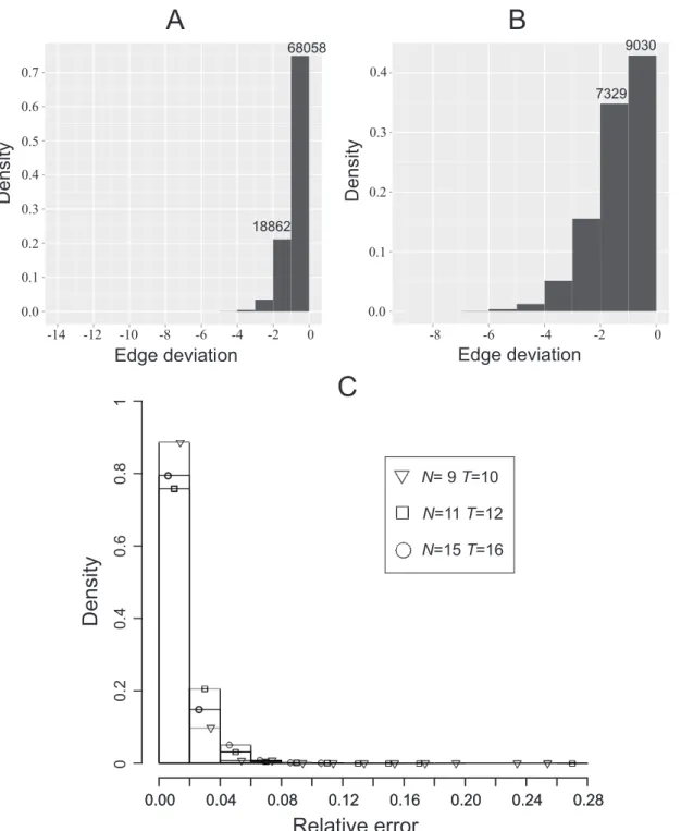
3.4. Validation of the algorithm for finding an approximated minimal network. To test the efficacy of the greedy heuristic, we constructed 90,635 feasible processes, each
withN~11and T~12. For each of these 90,635 processes, we
used the algorithm to seek an approximated minimal network. As a comparison, we also compute the actual minimal networks, by time-consuming brute force enumerations, whereby we can assess how far off from optimal the heuristic’s solutions are. The results are shown in Fig. 2(A). One sees that the approximated minimal network for each of the 68,058 processes (75.1% of total) is a genuine minimal network. The approximated minimal network for each of 18,862 processes (20.8% of total) has only one more edge than the genuine minimal network. Only 4% processes have two or more edges than minimal.
We also constructed 21,000 feasible processes each withN~15
andT~16. The results for these are shown in Fig. 2(B). One sees
that the approximated minimal network for each of the 9030 processes (43% of total) is a genuine minimal network. The approximated minimal network for each of the 7329 processes (34.9% of total) has one more edge than the genuine minimal network. Only 22% processes give deviations more than one edge.
We also studied manyN~9andT~10processes, with the results
presenting in Fig. 2(C), together with the other results.
The above numerical results indicate that the heuristic algorithm is very accurate, with high confidence for at most one additional edge than optimal.
File S1 F and G further provide examples of finding minimal networks.
4. Designability: How Many Solutions?
We consider one more computational aspect of Boolean
networks: computing thedesignabilityof a biological process. The
designability of a process is the number of network solutions, that is, the total number of networks that can produce a given process. A process with high designability is likely to be more robust and therefore survive natural selection. If a biological process has only one network solution, for example, then it is unlikely that random mutation would find that network. In other words, processes with high designability are more likely to occur (or be discovered by evolution) than low-designability ones [5,65].
problems [66]. Instead, we seek a fast approximate algorithm. Our approach is to use a type of logistic regression on certain features of a problem. These features are obtained during the simplification procedure described earlier in the feasibility solution.
During simplification, it is easy to obtain the following:xr, the
number of inhibitory edges (rji~1);xg, the number of stimulatory
edges (gji~1);xr, the number of edges that cannot be inhibitory
(rrji~1);xg, the number of edges that cannot be stimulatory (ggji~1); x0, the number of nodes that cannot connect to nodei(rrjiggji~1);
x1, the number of nodes that can be associated with nodei in
arbitrary way (inhibitory, stimulatory, or ‘‘no connection’’). We now assume that the approximated log-designability
(denoted byD) is a linear function ofxk:
Edge deviation
Edge deviation
Density
Density
A
68058
18862 0.7
0.6
0.5
0.4
0.3
0.2
0.1
0.0
0.4
0.3
0.2
0.1
0.0
-8 -6 -4 -2 0
-14 -12 -10 -8 -6 -4 -2 0
9030
7329
C
Relative error
Density
0.00 0.04 0.08 0.12 0.16 0.20 0.24 0.28
00
.2
0
.4
0.6
0.8
1
0.00 0.04 0.08 0.12 0.16 0.20 0.24 0.28
N
= 9 =10
T
N
=11 =12
T
N
=15 =16
T
B
Figure 2. Validation of a heuristic algorithm for finding an approximated minimal network.A large number of feasible Boolean processes
were generated. For each process, an approximated minimal network was determined by the heuristic algorithm; the actual minimal network is also computed by time-consuming enumeration. The histogram shows how the number of processes spread over the deviation of estimation (actual minimality minus estimated minimality). (A) 90,635 processes withN~11andT~12. (B) 21,000 processes withN~15andT~16. (C) Processes with N~9andT~10as compared with other processes.
lnD~bzX k
akxk, ð24Þ
where k[fr,g,rr,gg,0,1g, band ak are unknown coefficients. The
coefficients can be estimated by minimizing the difference between
the approximated designabilityDand the exact designabilityD0for
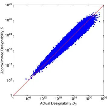
some test cases. To this end, we generate 800,000 random Boolean
process, each of which hasN~11andT~12. For each process, we
calculate the exact designability D0 and the values of xk, for
k[fr,g,rr,gg,0,1g. We then perform a least-square data fitting to
obtain the values of the coefficients. The results are:b~64:0796,
ar~{0:458234, ag~{0:302389, ar~{0:0477189, ag~ {0:0368327,a0~{0:572591, anda1~0:398622.
In Fig. (3), each dot represents one Boolean process; thexandy
axes representD0andD, respectively. One sees that the fitting is
successful. The dots locate along the diagonal with only small deviations. Therefore, we now have an empirical formula to estimate designability with sensible accuracy. Although it is not
very accurate to assume N- and T- independent regression
coefficients and use them to estimate designability, the estimation can still be very useful because it becomes very difficult to compute
the exact designability for largeNandT.
Discussion
Biological systems are generally large, involving many compli-cated molecular interactions among numerous working compo-nents. In this case, a ‘‘coarse grained’’ description such as a Boolean network model is often a useful step towards understand-ing a system. Furthermore, a study of general Boolean networks may help elucidate network design principles in biological systems. The Boolean framework in this paper results in a single analytical equation (Eq. 2) to integrate the information about network structure (edge variables) and biological process (state variables). This has rendered the structure-function relationship tractable. When structural information is known, one can use Eq. (2) to study the dynamics and learn the biological function. When the process is known, one can use Eq. (2) to characterize the network space constrained by the process. When both information are partially known, Eq. (2) can still help enumerate the structure-function combinations.
In this paper, we have answered some key questions about the computational complexity of the network inference problem in Boolean networks that feature dominant inhibition. The first is the feasibility problem: is the solution space null? The second is the minimal network problem: what are the fundamental building blocks of the space, namely those networks with the least number of edges? The third is the designability problem: how big is the solution space if it is not null?
Fast algorithms provide the benefit of being able to study many types of processes and to explore the statistics of processes. For example, one is interested in what general features of a process make a process a biological one suited to evolution. Is it the case, for example, that a small minimal network acts as the core with additional edges accumulated during evolution, and does a large multiplicity help maintain stability against mutation?
Beyond a rigorous classification of problem complexity, the present study also offers accurate heuristic algorithms that run in polynomial time. This will be crucial for handling both large-scale datasets and the inevitable statistical noise. The former requires a well-controlled scaling as observed in these polynomial heuristics and the latter requires iterative applications of these algorithms for noise sampling on a trial-and-error basis.
Supporting Information
File S1 A collection of technical details.
(PDF)
Author Contributions
Conceived and designed the experiments: GW CZ RS YR. Performed the experiments: GW. Analyzed the data: GW HC CD CP. Contributed reagents/materials/analysis tools: GW. Wrote the paper: GW RS CZ.
References
1. Bornholdt S (2005) Less is more in modeling large genetic networks. Science 310: 449–451.
2. Kauffman SA (1993) The Origins of Order: Self-Organization and Selection in Evolution. Oxford: Oxford University Press.
3. Li F, Long T, Lu Y, Ouyang Q, Tang C (2004) The yeast cell-cycle network is robustly designed. Proc Natl Acad Sci USA 101: 4781–4786.
4. Lau K, Ganguli S, Tang C (2007) Function constrains network architecture and dynamics: A case study on the yeast cell cycle Boolean network. Phys Rev E 75: 051907.
5. Nochomovitz YD, Li H (2006) Highly designable phenotypes and mutational buffers emerge from a systematic mapping between network topology and dynamic output. Proc Natl Acad Sci USA 103: 4180–4185.
6. Kashtan N, Alon U (2005) Spontaneous evolution of modularity and network motifs. Proc Natl Acad Sci USA 102: 13773–13778.
7. Emmert-Streib F (2010) A brief introduction to complex networks and their analysis. In: Dehmer M, editor, Structural Analysis of Complex Networks, New York: Birkha¨user. 1–26.
8. Estrada E (2011) The Structure of Complex Networks: Theory and Applications. Oxford: Oxford University Press.
Figure 3. Designability approximation.The 800,000 dots in the
picture each represent a random Boolean process. For each dot, the actual designability D0 and the approximated designability D are
represented by thexaxis value and theyaxis value, respectively. The diagonal corresponds to the ideal fitting.
9. Erdo¨s P, Re´nyi A (1959) On random graphs. Publicationes Mathematicae 6: 290–297.
10. Watts DJ, Strogatz SH (1998) Collective dynamics of small-world networks. Nature 393: 440–442.
11. Barabasi AL, Albert R (1999) Emergence of scaling in random networks. Science 286: 509–512.
12. Bornholdt S, Schuster HG (2003) Handbook of graphs and networks: from the genome to the internet. New York: Wiley.
13. Emmert-Streib F, Dehmer M (2007) Information theoretic measures of UHG graphs with low computational complexity. Appl Math Comput 190: 17831794. 14. Dehmer M, Emmert-Streib F (2008) Structural information content of networks: graph entropy based on local vertex functionals. Comput Biol Chem 32: 131– 138.
15. Dehmer M, Borgert S, Emmert-Streib F (2008) Entropy bounds for hierarchical molecular networks. PLoS ONE 3: e3079.
16. Dehmer M, Varmuza K, Borgert S, Emmert-Streib F (2009) On entropy-based molecular descriptors: Statistical analysis of real and synthetic chemical structures. J Chem Inf Model 49: 1655–1663.
17. Milo R, Shen-Orr S, Itzkovitz S, Kashtan N, Chklovskii D, et al. (2002) Network motifs: simple building blocks of complex networks. Science 298: 824–827. 18. Jeong H, Tombor B, Albert R, Oltvai ZN, Baraba´si AL (2000) The large-scale
organization of metabolic networks. Nature 407: 651–654.
19. Greenbury SF, Johnston IG, Smith MA, Doye JP, Louis AA (2010) The effect of scale-free topology on the robustness and evolvability of genetic regulatory networks. J Theor Biol 267: 48–61.
20. Bansal M, Belcastro V, Ambesi-Impiombato A, di Bernardo D (2007) How to infer gene networks from expression profiles. Mol Syst Biol 3: 78.
21. D’haeseleer P, Liang S, Somogyi R (2000) Genetic network inference: from co-expression clustering to reverse engineering. Bioinformatics 16: 707–726. 22. Shmulevich I, Zhang W (2002) Binary analysis and optimization-based
normalization of gene expression data. Bioinformatics 18: 555–565. 23. Needham CJ, Manfield IW, Bulpitt AJ, Gilmartin PM, Westhead DR (2009)
From gene expression to gene regulatory networks in arabidopsis thaliana. BMC Syst Biol 3: 85.
24. Altay G, Emmert-Streib F (2011) Structural influence of gene networks on their inference: analysis of C3NET. Biol Direct 6: 31.
25. Ideker T, Thorsson V, Karp R (2000) Discovery of regulatory interactions through perturbation: inference and experimental design. In: Pacific Symposium on Biocomputing. World Scientific Maui, Hawaii, volume 5, 302–313. 26. Akutsu T, Kuhara S, Maruyama O, Miyano S (2003) Identification of genetic
networks by strategic gene disruptions and gene overexpressions under a Boolean model. Theor Comput Sci 298: 235–251.
27. Perkins T, Hallett M (2010) A trade-off between sample complexity and computational complexity in learning Boolean networks from time-series data. IEEE/ACM Trans Comput Biol Bioinform 7: 118–125.
28. Saithong T, Bumee S, Liamwirat C, Meechai A (2012) Analysis and practical guideline of constraint-based Boolean method in genetic network inference. PLoS ONE 7: e30232.
29. Wang G, Du C, Simha R, Rong Y, Xiao Y, et al. (2010) Process-based network decomposition reveals backbone motif structure. Proc Natl Acad Sci U S A 107: 10478–10483.
30. Albert R, Othmer HG (2003) The topology of the regulatory interactions predicts the expression pattern of the segment polarity genes in Drosophila melanogaster. J Theor Biol 223: 1–18.
31. Kauffman S (1969) Metabolic stability and epigenesis in randomly constructed genetic nets. J Theor Biol 22: 437–467.
32. Glass L, Kauffman S (1973) The logical analysis of continuous, non-linear biochemical control networks. J Theor Biol 39: 103–129.
33. Tan N, Ouyang Q (2006) Design of a network with state stability. J Theor Biol 240: 592–598.
34. Fortuna MA, Melia´n CJ (2007) Do scale-free regulatory networks allow more expression than random ones? J Theor Biol 247: 331–336.
35. Chandru V, Coullard CR, Hammer PL, Montanez M, Sun X (1990) On renamable Horn and generalized Horn functions. Ann Math Artif Intell 1: 33– 47.
36. Dowling WF, Gallier JH (1984) Linear time algorithms for testing the satisfiability of propositional Horn formulae. J Logic Program 1: 267–284.
37. Alon U (2003) Biological networks: the tinkerer as an engineer. Science 301: 1866–1867.
38. Mendelson E (1997) Introduction to Mathematical Logic. London: Chapman and Hall.
39. Brassard G, Bratley P (1996) Fundamentals of Algorithmics. Prentice Hall. 40. Cook SA (1971) The complexity of theorem-proving procedures. In: Proceedings
of the third annual ACM symposium on Theory of computing. ACM, 151–158. 41. Aspvall B, Plass MF, Tarjan RE (1979) A linear-time algorithm for testing the truth of certain quantified Boolean formulas. Inform Process Lett 8: 121–123. 42. Horn A (1951) On sentences which are true of direct unions of algebras. J Symb
Logic 16: 14–21.
43. Chang CC, Morel AC (1958) On closure under direct product. J Symb Logic 23: 149–154.
44. Keisler HJ (1965) Reduced products and Horn classes. Trans Amer Math Soc 117: 307–328.
45. Cook S, Nguyen P (2010) Logical foundations of proof complexity. Cambridge: Cambridge University Press.
46. Perkins TJ, Wilds R, Glass L (2010) Robust dynamics in minimal hybrid models of genetic networks. Phil Trans R Soc A 368: 4961–4975.
47. Finlayson MR, Helfer-Hungerbu¨hler AK, Philippsen P (2011) Regulation of exit from mitosis in multinucleate ashbya gossypii cells relies on a minimal network of genes. Mol Biol Cell 22: 3081–3093.
48. Howes R, Eccleston L, Gonalves J, Stan GB,Warnick S (1998) Dynamical structure analysis of sparsity and minimality heuristics for reconstruction of biochemical networks. In: Proceedings of the 47th IEEE Conference on Decision and Control. IEEE, Cancun, Mexico: IEEE.
49. Raychaudhuri S (2010) A minimal model of signaling network elucidates cell-to-cell stochastic variability in apoptosis. PLoS ONE 5: e11930.
50. Okazaki N, Asano R, Kinoshita T, Chuman H (2008) Simple computational models of type I/type II cells in Fas signaling-induced apoptosis. J Theor Biol 250: 621–633.
51. van Beek P, Dechter R (1995) On the minimality and global consistency of row-convex constraint networks. J ACM 42: 543–561.
52. Blum A, Langley P (1997) Selection of relevant features and examples in machine learning. Artif Intell 97: 245–271.
53. Mossel E, O’Donnell R, Servedio RP (2003) Learning juntas. In: Proceedings of the thirty-fifth annual ACM symposium on Theory of computing. ACM, 206– 212.
54. Mukherjee S, Pelech S, Neve RM, Kuo WL, Ziyad S, et al. (2009) Sparse combinatorial inference with an application in cancer biology. Bioinformatics 25: 265–271.
55. Hogan JM, Diederich J (2001) Recruitment learning of Boolean functions in sparse random networks. Int J Neural Syst 11: 537–559.
56. Fukagawa D, Akutsu T (2005) Performance analysis of a greedy algorithm for inferring Boolean functions. Inform Process Lett 93: 7–12.
57. Chvatal V (1979) A greedy heuristic for the set-covering problem. Math Oper Res 4: 233–235.
58. Garey MR, Johnson DS (1979) Computers and Intractability: A Guide to the Theory of NP-Completeness. New York: W.H. Freeman.
59. Alon N, Moshkovitz D, Safra S (2006) Algorithmic construction of sets for k-restrictions. ACM Trans Algorithms 2: 153–177.
60. Karp RM (1972) Reducibility among combinatorial problems. In: Miller RE, Thatcher JW, editors, Complexity of Computer Computations, New York: Plenum. 85–103.
61. Chvatal V (1979) A greedy heuristic for the set covering problem. Math Oper Res 4: 233–235. 22
62. Kosaraju SR, Scha¨ffer AA, Biesecker LG (1998) Approximation algorithms for a genetic diagnostics problem. J Comput Biol 5: 9–26.
63. Doi K, Imai H (1997) Greedy algorithms for finding a small set of primers satisfying cover and length resolution conditions in PCR experiments. Genome Inform Ser Workshop Genome Inform 8: 43–52.
64. Chowdhury SA, Koyut¨urk M (2010) Identification of coordinately dysregulated subnetworks in complex phenotypes. Pac Symp Biocomput 15: 133–144. 65. Isalan M, Lemerle C, Michalodimitrakis K, Horn C, Beltrao P, et al. (2008)
Evolvability and hierarchy in rewired bacterial gene networks. Nature 452: 840– 845.