Response of halocarbons to ocean acidification in the Arctic

(1)

BGD

9, 8199–8239, 2012

Response of halocarbons to ocean

acidification in the Arctic

F. E. Hopkins et al.

Title Page

Abstract Introduction

Conclusions References

Tables Figures

◭ ◮

Back Close

Full Screen / Esc

Printer-friendly Version Interactive Discussion

Discussion

P

a

per

|

Dis

cussion

P

a

per

|

Discussion

P

a

per

|

Discussio

n

P

a

per

|

Biogeosciences Discuss., 9, 8199–8239, 2012 www.biogeosciences-discuss.net/9/8199/2012/ doi:10.5194/bgd-9-8199-2012

Biogeosciences Discussions

This discussion paper is/has been under review for the journal Biogeosciences (BG). Please refer to the corresponding final paper in BG if available.

Response of halocarbons to ocean

acidification in the Arctic

F. E. Hopkins1, S. A. Kimmance1, J. A. Stephens1, R. G. J. Bellerby2,3,4, C. P. D. Brussaard5, J. Czerny6, K. G. Schulz6, and S. D. Archer1,7

1

Plymouth Marine Laboratory, Plymouth, UK

2

Norwegian Institute for Water Research, Bergen, Norway

3

Uni Bjerknes Centre, Uni Research AS, Bergen, Norway

4

Geophysical Institute, University of Bergen, Bergen, Norway

5

Royal Netherlands Institute for Sea Research (NIOZ), Texel, The Netherlands

6

Helmholtz Centre for Ocean Research (GEOMAR), Kiel, Germany

7

Bigelow Laboratory for Ocean Sciences, Maine, USA

Received: 24 May 2012 – Accepted: 25 May 2012 – Published: 9 July 2012

Correspondence to: F. E. Hopkins (fhop@pml.ac.uk)

(2)

BGD

9, 8199–8239, 2012

Title Page

Tables Figures

◭ ◮

Back Close

Full Screen / Esc

Discussion

P

a

per

|

Dis

cussion

P

a

per

|

Discussion

P

a

per

|

Discussio

n

P

a

per

Abstract

The potential e_ffect of ocean acidification (OA) on seawater halocarbons in the Arc-tic was investigated during a mesocosm experiment in Spitsbergen in June–July 2010. Over a period of 5 weeks, natural phytoplankton communities in nine ∼50 m3

mesocosms were studied under a range of pCO₂ treatments from _∼185 µatm to

5

∼1420 µatm. In general, the response of halocarbons to pCO2 was subtle, or

unde-tectable. A large number of significant correlations with a range of biological parame-ters (chlorophylla, microbial plankton community, phytoplankton pigments) were iden-tified, indicating a biological control on the concentrations of halocarbons within the mesocosms. The temporal dynamics of iodomethane (CH₃I) alluded to active turnover

10

of this halocarbon in the mesocosms and strong significant correlations with biological parameters suggested a biological source. However, despite apCO₂e_ffect on various

components of the plankton community, and a strong association between CH₃I and

biological parameters, no effect of pCO₂ was seen in CH₃I. Diiodomethane (CH₂I₂) displayed a number of strong relationships with biological parameters. Furthermore,

15

the concentrations, the rate of net production and the sea-to-air flux of CH₂I₂showed a significant positive response topCO₂. There was no clear effect ofpCO₂ on carbon concentrations or dynamics. However, periods of significant net loss of bromo-form (CHBr₃) were found to be concentration-dependent, and closely correlated with total bacteria, suggesting a degree of biological consumption of this halocarbon in

Arc-20

(3)

BGD

9, 8199–8239, 2012

Title Page

Tables Figures

◭ ◮

Back Close

Full Screen / Esc

Discussion

P

a

per

|

Dis

cussion

P

a

per

|

Discussion

P

a

per

|

Discussio

n

P

a

per

|

1 Introduction

Volatile marine halocarbons are produced via a range of biological and photochemical processes in the surface ocean, resulting in a strong flux to the marine atmosphere. Production processes include direct biological synthesis by phytoplankton, bacteria and macroalgae (Tokarczyk and Moore, 1994; Tait and Moore, 1995; Moore et al., 1996;

5

Manley and Cuesta, 1997; Scarratt and Moore, 1998; Amachi et al., 2001; Hughes et al., 2006), and indirect production through reactions between dissolved organic matter and light (Moore and Zafiriou, 1994; Happell and Wallace, 1996; Richter and Wallace, 2004) and/or ozone (Martino et al., 2009). Seawater concentrations of halo-carbons are also controlled by a number of loss processes, including hydrolysis and

10

nucleophilic attack (Zafiriou, 1975; Elliott and Rowland, 1993), photolysis (Jones and Carpenter, 2005; Martino et al., 2005) and bacterial assimilation (King and Saltzman, 1997; Goodwin et al., 1998, 2001). The resultant surface ocean halocarbon pool under-goes sea-air gas exchange, a flux which constitutes the most important source of nat-ural halogens to the atmosphere. Halocarbons are rapidly oxidised in the atmosphere

15

to produce reactive radicals (I, IO, Br, BrO) which exert an important control on ozone (Chameides and Davis, 1980; Solomon et al., 1994; Davis et al., 1996; Read et al., 2008), and act as condensation nuclei for the growth of larger particles and clouds with the potential to influence global climate (O’Dowd et al., 2002).

In the Arctic, atmospheric halogen species are implicated in ozone (O₃) depletion

20

events (ODEs) – dramatic losses of tropospheric ozone that occur following the po-lar sunrise. ODEs are initiated and catalysed by photochemistry that converts inert halide salt ions (e.g. Br−_{) into reactive halogen species (e.g., Br and BrO). The most}

extensive ODEs occur over the frozen Arctic Ocean, as sea-ice surfaces, brine and frost flowers represent the main source of inorganic bromine during these events (see

25

(4)

BGD

9, 8199–8239, 2012

Title Page

Tables Figures

◭ ◮

Back Close

Full Screen / Esc

Discussion

P

a

per

|

Dis

cussion

P

a

per

|

Discussion

P

a

per

|

Discussio

n

P

a

per

such as diiodomethane (CH₂I₂) have a significantly greater O₃ depletion effect (per molecule) than the addition of further sea-salt derived Br₂/BrCl (Calvert and Lindberg, 2004). Recent work in sub-Arctic Canada has further raised the importance of halocar-bons in Arctic atmospheric chemistry. A combination of Differential Optical Absorption Spectroscopy (DOAS) observations of IO and measurements of atmospheric mixing

5

ratios of halocarbons has revealed episodes of elevated IO, accompanied by a variety of iodocarbons (Mahajan et al., 2010). Air-mass back trajectories show that the iodine compounds originated from open water polynyas in the sea-ice covered Hudson Bay. Using the one-dimensional Tropospheric Halogen Chemistry Model (THAMO) (Saiz-Lopez et al., 2008), Mahajan et al. showed that iodocarbon sources from ice-free Arctic

10

waters could account for the observed concentrations of IO. Such levels of IO deplete O₃at rates comparable to BrO. Furthermore, relatively small amounts of IO can cause a large increase in the O₃destruction potential of BrO.

The Arctic region is currently experiencing rapid environmental change. Summer sea-ice extent has steadily decreased over the past 30 yr, and the rate of this decline

15

now exceeds any predictions made using IPCC AR4 simulations (Stroeve et al., 2011; Wang and Overland, 2009). The duration of melt season has increased by about 20 days over the last 30 yr for the Arctic as a whole (Markus et al., 2009), and in areas where sea ice concentration has decreased in early summer, the timing of the annual phytoplankton blooms has become significantly earlier (Kahru et al., 2011 ). The Arctic

20

region is particularly susceptible to ocean acidification (OA). Over 400 billion tons of CO₂has been released to the atmosphere by human activities over the last 200 yr, one third of which has been soaked up by the oceans (Calderia and Wickett, 2003; Sabine et al., 2004). This unprecedented influx of CO₂ is resulting in an increase in H+ ion concentrations manifested as a drop in surface ocean pH, accompanied by a decrease

25

in the saturation state of calcium carbonate (ΩCaCO₃). This reduces the availability of carbonate ions (CO2−

3 ) which are a vital component of the skeletons of calcifying

(5)

BGD

9, 8199–8239, 2012

Title Page

Tables Figures

◭ ◮

Back Close

Full Screen / Esc

Discussion

P

a

per

|

Dis

cussion

P

a

per

|

Discussion

P

a

per

|

Discussio

n

P

a

per

|

predictions suggest that areas of the surface Arctic Ocean will, within the next decade, be the first to experience the e_ffects of OA (Steinacher et al., 2009).

Recently, there has been interest in how the changing Arctic climate may influence the sea-to-air flux of halocarbons. Declining sea ice extent and thickness, accompanied by an increase in open water and marine primary productivity, could result in an

up-5

turn in the net production and resulting flux of halocarbons to the atmosphere (Mahajan et al., 2010; Shaw et al., 2011; Zhang et al., 2010). This may elevate the importance of halocarbons in Arctic atmospheric chemistry and O₃ regulation. However, nothing is known of the response of marine halocarbons to OA in the Arctic, a phenomenon that will go hand-in-hand with climatic changes. Species shifts in phytoplankton (see

10

Riebesell and Tortell, 2011 for review) and increased rates of bacterial activity (Piontek et al., 2010) are anticipated responses to future OA. Furthermore, different species of phytoplankton are known to produce differing quantities of halocarbons. Therefore, in order to gain an understanding of the future flux of marine halocarbons to the atmo-sphere, a whole ecosystem approach must be adopted and mesocosm experiments

15

provide this vital platform.

Previous mesocosm experiments performed in Norwegian temperate coastal waters have given contrasting e_ffects of OA on halocarbons. Wingenter et al. (2007) observed

large increases in chloroiodomethane (CH₂ClI) under 2× ambient CO2 (46±4 %)

and 3× ambient CO2 (131±11 %) relative to ambient control mesocosms. By

con-20

trast, Hopkins et al. (2010) reported large and significant decreases in a variety of iodocarbons under high CO₂(∼750 µatm) relative to present day control mesocosms (∼380 µatm), whilst the bromocarbons showed little response to the future conditions. Now, we need to understand how the net production of halocarbons from other ocean regions may respond to OA. As marine halocarbons may be key players in Arctic

at-25

(6)

BGD

9, 8199–8239, 2012

Title Page

Tables Figures

◭ ◮

Back Close

Full Screen / Esc

Discussion

P

a

per

|

Dis

cussion

P

a

per

|

Discussion

P

a

per

|

Discussio

n

P

a

per

2 Materials and methods

2.1 General experimental set-up

A mesocosm experiment was performed between 31 May and 7 July 2010 in Kongsfjor-den (78◦_56.2′_{N; 11}◦_53.6′_{E), on the west coast of Spitsbergen, the largest island of the}

Svalbard Archipelago. A total of nine mesocosms were deployed in the fjord, moored

5

in sets of three with∼40 m between each mesocosm and ∼50 m between the triplets, and each capable of enclosing_∼50 m3 of seawater. The mesocosms were filled with fjord water which was screened through 3 mm mesh to eliminate larger organisms in-cluding pteropods. On 2 June (t₋₅), the mesocosms were closed, allowing no further exchange with the surrounding fjord water. The mesocosms were fully open to the

at-10

mosphere, but were covered with a transparent protective lid to minimise external nutri-ent inputs from seabirds and rain. Seven of the mesocosms received varying amounts of CO₂-saturated seawater over a period of 5 days (t₋₁ tot₄), resulting in a range of pCO₂levels, from∼185 to 1420 µatm (Phase 0). The two control mesocosms received no CO₂ addition, and represented the in situ carbonate chemistry of the fjord (175–

15

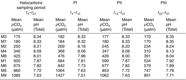
180 µatm). Once thepCO₂/pH levels had been adjusted, daily experimental sampling of the mesocosms for halocarbons began, commencing on 11 June (t₄) and continuing until 4 July (t27). Table 1 gives a summary of the meanpCO2(µatm) and pH (on the

total scale) for the period t₄–t₂₇, as well as mean values for the three experimental phases that are referred to in this paper. Nutrients were added to the mesocosms on

20

20 June (t13) (mean concentrations: nitrate 5.56 µM, phosphate 0.39 µM, and silicate

(7)

BGD

9, 8199–8239, 2012

Title Page

Tables Figures

◭ ◮

Back Close

Full Screen / Esc

Discussion

P

a

per

|

Dis

cussion

P

a

per

|

Discussion

P

a

per

|

Discussio

n

P

a

per

|

2.2 Sampling for halocarbon compounds

Samples for halocarbon analysis were taken using a depth integrating water sampler (IWS) (Hydrobios, Kiel, Germany) deployed from a small boat, suitable for the collec-tion of trace gas-sensitive samples. The sampler was manually lowered through the water column to depth, and programmed to collect a 12 m-integrated sample. Once

re-5

turned to the boat, a length of Tygon tubing was attached to the outlet at the bottom of the sampler and sub-samples for halocarbon analysis were collected in 250 ml amber glass-stoppered bottles. The bottle was rinsed three times before the Tygon tubing was placed to the bottom of the bottle, allowing it to gently fill and overflow three times. On the fourth filling, the bottle was filled to the top and the glass-stopper was replaced,

10

ensuring the absence of bubbles or headspace. Samples were transported in a cool box back to the laboratory onshore, and all were analysed within 6 h of collection.

2.3 Quantification of halocarbons compounds

Seawater sub-samples were gently withdrawn from the amber glass-stoppered bottles using a 100 ml glass syringe and 1/8′′nylon syringe extension. The sample was filtered

15

through a 0.7 µm filter (GF/F, Whatman) into a second syringe, ensuring that the intro-duction of bubbles into the samples was avoided at all times. Following the addition of two deuterated surrogate analytes to monitor instrument sensitivity drift (Martino et al., 2005; Hughes et al., 2006), a 40 ml sample was injected into a glass purge vessel, and the halocarbons were extracted by purging the seawater with ultra-high purity (BIP)

ni-20

trogen for 10 min at a flow rate of 90 ml min−1_{. Aerosols were removed from the purge}

gas stream using glass wool contained within a section of glass tubing, and a coun-terflow nafion drier using oxygen-free nitrogen at a flow rate of 180 ml min−1_{was used}

to dry the gas. Halocarbons were trapped on triple-bed stainless steel solid sorbent tubes (Markes International Ltd.) containing Tenax, Carbograph and Carboxen, held

25

at 1–2◦_{C in a custom-made peltier-cooled metal block. Sample tubes were analysed}

(8)

BGD

9, 8199–8239, 2012

Title Page

Tables Figures

◭ ◮

Back Close

Full Screen / Esc

Discussion

P

a

per

|

Dis

cussion

P

a

per

|

Discussion

P

a

per

|

Discussio

n

P

a

per

Gas Chromatograph-Mass Spectrometer (GC-MS), coupled to a Markes Unity thermal desorption (TD) platform. The GC was fitted with a 60 m DB-VRX capillary column (0.32 µm film thickness, J & W Ltd.), and the MS was operated in electron ionization (EI)/single ion mode (SIM) throughout the analyses. Within Unity, the sample tubes

were heated to 200◦_{C for 5 min, and the desorbed sample was refocused on a cold}

5

trap held at−10◦C. Following this, the cold trap underwent rapid heating up to 290◦C at a rate of 100◦C s−1 and the sample was introduced to the GC column using a He carrier flow rate of 2 ml min−1_{. The GC oven was held at 40}◦_{C for 5 min, then heated}

to 200◦C at a rate of 20◦C min−1 and held for 2 min. Finally the oven was heated to 240◦C at a rate of 20◦C min−1 and held for 4 min. The total run time was 21 min, and

10

the MS collected data between 6 and 14 min of the run. Calibration and quantification of the compounds was performed using laboratory-prepared liquid standards, by dilution of the pure compounds into ultra-high purity methanol. The primary standards were prepared gravimetrically, the secondary and working standards by serial dilution. The analytical error as based on triplicate samples were: <5 % for Iodomethane (CH₃I),

15

2-iodopropane (2-C₃H₇I), 1-iodopropane (1-C₃H₇I), chloroiodomethane (CH₂ClI), bro-moiodomethane (CH₂BrI), <10 % for CH₂I₂, bromoform (CHBr₃), dibromomethane (CH₂Br₂), dibromochloromethane (CHBr₂Cl), and 10–15 % for Iodoethane (C₂H₅I), bromochloromethane (CH₂BrCl).

2.4 Sea-to-air flux of halocarbons

20

The sea-to-air flux of halocarbons, determined by the concentration difference be-tween the air and seawater after correcting for solubility, was estimated for all meso-cosms. Gas exchange in the mesocosms was determined by the addition of 3 times-atmospheric concentrations of N₂O and the measurement of the subsequent loss rates, allowing the transfer velocity (k) of N₂O to be derived and enabling the estimation of the

25

(9)

BGD

9, 8199–8239, 2012

Title Page

Tables Figures

◭ ◮

Back Close

Full Screen / Esc

Discussion

P

a

per

|

Dis

cussion

P

a

per

|

Discussion

P

a

per

|

Discussio

n

P

a

per

|

(2012, this issue). Transfer velocities of halocarbons (k_halo) were derived as follows:

k_halo=k_N₂_O/(Sc_halo/Sc_N₂_O)0.5 (1)

The Schmidt number of halocarbons (Sc_halo) was estimated based on experimentally-determined values of molecular diffusivity for CH₃Br (De Bruyn and Saltzman, 1997), using an approach described by Moore and Groszko (1999). Estimated fluxes of

halo-5

carbons could then be calculated, using experimentally determined values of the di-mensionless Henry’s Law Coe_fficient (Moore et al., 1995), and the only reported

at-mospheric concentrations of halocarbons from Ny- ˚Alesund reported by Schall and

Heumann (1993). Fluxes were low relative to open ocean measurements due to the sheltered nature of the mesocosm environment and a minimal wind speed component

10

(see Czerny et al., 2012, this issue).

2.5 Ancillary measurements

2.5.1 Chlaand additional phytoplankton pigments

Samples for both chlaand additional phytoplankton pigments were processed as soon as possible after sampling, and in the meantime, were stored at the in situ temperature

15

of the fjord. For chla500 ml of seawater was filtered onto GF/F filters (Whatman), and immediately frozen and stored at₋20◦_{C. Chl}_a_{was measured after a minimum of 24 h}

in the freezer, and extraction was performed with 10 ml acetone (90 %). The filter was homogenised for 4 min with 5 ml acetone, after which an additional 5 ml was added and the sample centrifuged. The supernatant was then analysed fluorometrically after

20

the method of Welschmeyer (1994). For determination of the individual phytoplankton pigments, 2×750 ml were filtered, which was reduced to 1×750 ml at the onset of the bloom. The filters were immediately frozen and stored at−80◦C until analysis at GEOMAR. Pigments were extracted with 3 ml acetone and analysed using high pres-sure liquid chromatography (HPLC), with the addition of Canthaxanthin as an internal

25

(10)

BGD

9, 8199–8239, 2012

Title Page

Tables Figures

◭ ◮

Back Close

Full Screen / Esc

Discussion

P

a

per

|

Dis

cussion

P

a

per

|

Discussion

P

a

per

|

Discussio

n

P

a

per

2.5.2 Microbial abundance

Samples for the quantification of the microbial plankton community were taken directly from the integrated water sampler from the same cast used to collect the halocarbon samples, thus providing plankton counts that were directly comparable to halocarbon concentrations.

5

2.5.3 Phytoplankton abundance and composition

Phytoplankton composition and abundance were determined by analysis of fresh sam-ples on a Becton Dickinson FACSort flow cytometer (FCM) equipped with a 15 mW laser exciting at 488 nm and with a standard filter set up. Samples were analysed at high flow rate (∼150 µl min−1), and specific phytoplankton groups were discriminated

10

in bivariate scatter plots by differences in side scatter and red-orange fluorescence (Tarran et al., 2001).

2.5.4 Total bacteria abundance

Samples for bacterial enumeration were fixed for 30 min at 7◦C with glutaraldehyde (25 %, EM-grade) at a final concentration of 0.5 % before snap freezing in liquid

nitro-15

gen and storage at₋80◦_{C until analysis. Bacteria were counted using a FCM}

accord-ing to Marie et al. (1999). Briefly, thawed samples were diluted with Tris-EDTA buffer (10 mM Tris-HCl and 1 mM EDTA, pH 8) and stained with the green fluorescent nucleic acid-specific dye SYBR-Green I (Molecular Probes, Invitrogen Inc.) at a final concen-tration of 1×10−4of the commercial stock, in the dark at room temperature for 15 min.

20

(11)

BGD

9, 8199–8239, 2012

Title Page

Tables Figures

◭ ◮

Back Close

Full Screen / Esc

Discussion

P

a

per

|

Dis

cussion

P

a

per

|

Discussion

P

a

per

|

Discussio

n

P

a

per

|

2.6 Statistical analyses

In order to identify differences in halocarbon concentrations between mesocosms, one-way analyses of variance (ANOVA) were applied to the data. Initially, tests of normality were applied (p <0.05₌not normal), and if data failed to fit the assumptions of the test, linearity transformations of the data were performed (logarithmic or square root),

5

and the ANOVA proceeded from this point. The results of ANOVA are given as follows: F =ratio of mean squares, df₌degrees of freedom,σ=significance ofF-test,p=level of confidence. For those data which still failed to display normality following transfor-mation, a rank-based Kruskal–Wallis test was applied (H=test statistic, df=degrees of freedom,p=level of confidence).

10

Relationships between halocarbons and a range of other parameters were investi-gated using Pearson’s correlation coefficients (R), along with the associated probability (F test,p <0.05=significant). Net loss and production rates of halocarbons were de-rived from linear regression analyses of halocarbon concentration data as a function of time, to give the rate coefficient (pmol l−1d−1), the coefficient of determination (R2),

15

the standard error (SE) of the rate and the associated level of confidence (F test, p <0.05₌significant).

3 Results

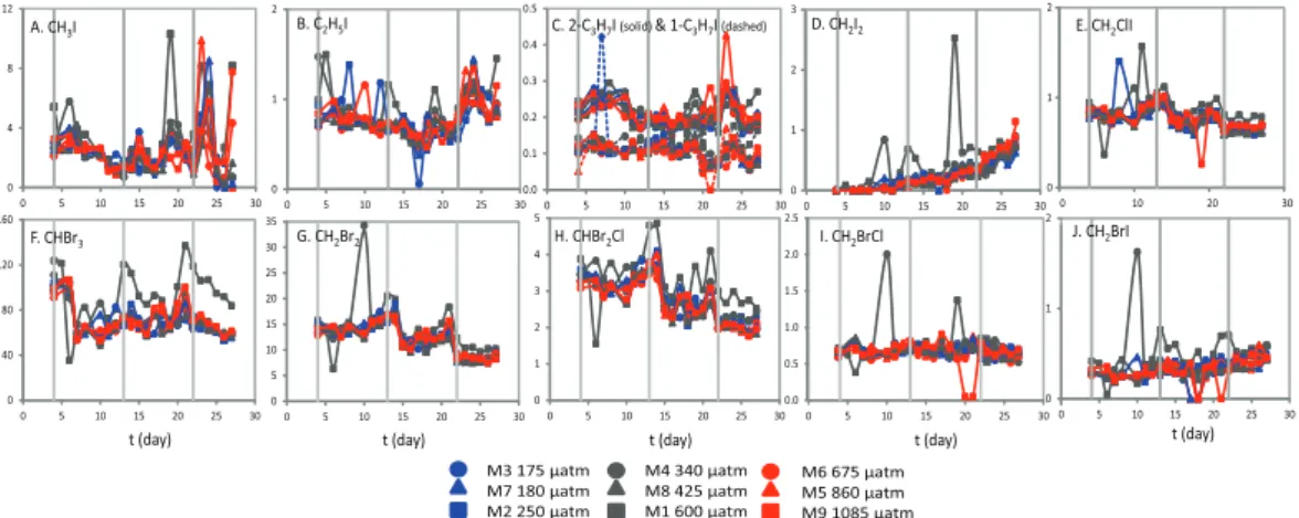
3.1 Halocarbon temporal dynamics

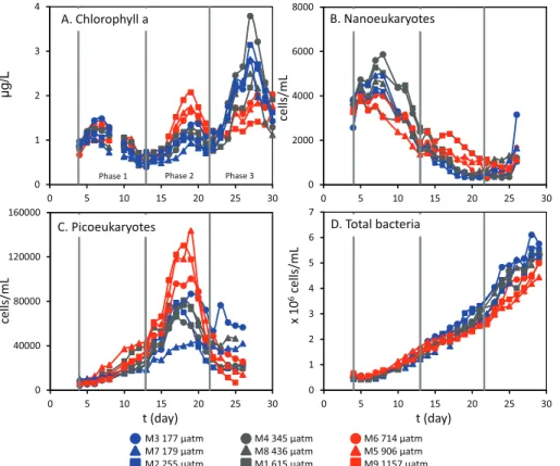
Data for chlorophyll a (chl a) and microbial plankton counts (nanoeukaryotes and

pi-20

coeukaryotes, total bacteria) are shown in Fig. 1, and concentrations of halocarbons are shown in Fig. 2. The experiment was divided into three phases (PI, PII, PIII) based on the addition of nutrients and the dynamics of chl a (see Schulz et al., 2012, this issue). The divisions between phases are indicated on the figures as grey vertical lines (see Table 1 for a summary of timings). Mean concentrations of all halocarbons

(12)

BGD

9, 8199–8239, 2012

Title Page

Tables Figures

◭ ◮

Back Close

Full Screen / Esc

Discussion

P

a

per

|

Dis

cussion

P

a

per

|

Discussion

P

a

per

|

Discussio

n

P

a

per

in the control mesocosms M3 and M7 were not significantly different from each other (Kruskal–Wallis ANOVA on ranks,p >0.05 for all halocarbons).

3.1.1 Iodocarbons

Concentrations of CH₃I and C₂H₅I (Fig. 2a, b) showed some variability over the course of the experiment, falling gradually during PI, in parallel to chl a oncentrations and

5

nanophytoplankton abundances. Peaks occurred following nutrient addition and in par-allel with the chla peak ont₁₉ in PII, and during the rapid rise in chla observed dur-ing PIII. Concentrations ranged from 0.04 to 10.29 pmol l−1 and 0.06 to 3.32 pmol l−1, for CH₃I and C₂H₅I, respectively. Concentrations of the propyl iodides (Fig. 2c) were less variable, with concentrations varying by less than 0.5 pmol l−1, and overall mean

10

concentrations of 0.21 pmol l−1 _(2-C

3H7I) and 0.12 pmol l−1 (1-C3H7I). However,

con-centrations did show some increase that coincided with the final chlamaximum in PIII. 2-C₃H₇I was consistently higher than 1-C₃H₇I by ∼0.1 pmol l−1. For all of the above and for the experiment as a whole, no significant differences in mean concentrations

were detected between mesocosms and no apparent e_ffect of pCO₂ were observed

15

(Kruskal–Wallis ANOVA on ranks (df=8): CH₃IH=6.06, p=0.64; C₂H₅IH =15.03, p=0.06; 2-C₃H₇IH=11.73,p=0.11; 1-C₃H₇IH =10.22,p=0.18).

In contrast to all other halocarbons, CH₂I₂ concentrations (Fig. 2d) gradually increased over the course of the experiment, from below detection limit (D.L., <10 fmol l−1) ont₄, reaching 0.5–1.0 pmol l−1by t₂₇. M1 displayed significantly higher

20

concentrations over almost the entire duration of the experiment, with a maximum

and seemingly anomalous value of 2.5 pmol l−1 on t₁₉ (ANOVA F =2.52, df=8,

σ=0.014, p <0.05). In PIII concentrations showed some response to pCO₂ treat-ment, with significantly higher mean CH₂I₂concentrations as a function of meanpCO₂ (R2=0.451, n=9, p <0.05). CH₂ClI concentrations (Fig. 2e) were generally stable

25

(13)

BGD

9, 8199–8239, 2012

Title Page

Tables Figures

◭ ◮

Back Close

Full Screen / Esc

Discussion

P

a

per

|

Dis

cussion

P

a

per

|

Discussion

P

a

per

|

Discussio

n

P

a

per

|

significantly topCO₂treatment, although concentrations in M1 were significantly higher

than M6, M7 and M8 (Kruskal–Wallis ANOVA on ranks H=22.19, df₌8, p=0.005,

pairwise comparison with Dunn’s method – allp <0.05).

3.1.2 Bromocarbons

The temporal development of concentrations of CHBr₃, CH₂Br₂and CHBr₂Cl (Fig. 2f–

5

h) showed a high degree of similarity, with a gradual rise fromt₆, a sharp drop at the start of PII followed by a period of recovery during the nutrient-induced chlapeak, and falling or unchanging concentrations during PIII. For the entire experiment the concen-trations of CHBr₃>CH₂Br₂>CHBr₂Cl with mean concentrations for all mesocosms of 72.8 pmol l−1, 12.4 pmol l−1 and 2.8 pmol l−1, respectively. Similarly to CH₂I₂,

concen-10

trations of CHBr₃, CH₂Br₂and CHBr₂Cl were almost consistently higher in M1 (signifi-cantly higher for CHBr₃Kruskal–Wallis ANOVA on ranksH=27.258, df₌8,p <0.001), although followed similar temporal trends to the other mesocosms. Concentrations of CH₂BrCl (Fig. 2i) were low (<0.1 pmol l−1_{) and stable, with the exception of a small}

number of anomalous data points in PI and PII. CH₂BrI showed little variability as

15

the experiment progressed (overall mean₌0.35 pmol l−1_{), with the exception of some}

anomalous spikes in concentration during PI and II, and little response to nutrient-addition or phytoplankton growth (Fig. 2j). No significant responses topCO₂were de-tected (Kruskall-Wallis ANOVA on ranks (df₌8): CHBr₃ H=3.94, p=0.86; CH₂Br₂ H=2.22, p=0.95; CH₂BrCl H=8.94, p=0.35; CHBr₂Cl H=4.84, p=0.68; CH₂BrI

20

H=10.67,p=0.16).

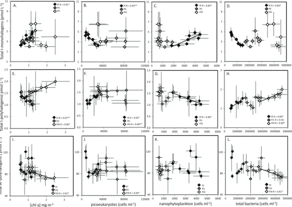
3.2 Halocarbons and biological parameters

In order to identify possible sources or sinks in the mesocosms, concentrations of halo-carbons were compared with a number of biological parameters (chla, nanoeukaryote and picoeukaryote abundance, and total bacteria abundance). To simplify these

analy-25

(14)

BGD

9, 8199–8239, 2012

Title Page

Tables Figures

◭ ◮

Back Close

Full Screen / Esc

Discussion

P

a

per

|

Dis

cussion

P

a

per

|

Discussion

P

a

per

|

Discussio

n

P

a

per

groups based on their common biological production pathways: (1) I-monohalocarbons (CH₃I, C₂H₅I, 2-C₃H₇I, 1-C₃H₇I), potentially formed via methyl transferase activity, (2) I-polyhalocarbons (CH₂I₂, CH₂ClI), potentially formed via iodoperoxidase activity, (3) Br-polyhalocarbons (CHBr₃, CH₂Br₂, CH₂BrCl, CHBr₂Cl, CH₂BrI), potentially formed via bromoperoxidase activity (compare Fig. 3). I-monohalocarbons showed the strongest

5

correlations with biological parameters during PI (Fig. 3a–d). Significant positive cor-relations were identified with both chlaand nanophytoplankton (Fig. 3a, c, whilst sig-nificant negative correlations were observed with picoeukaryotes and total bacteria (Fig. 3b, d). No significant correlations were observed during PII and PIII. PI also re-vealed a number of strong relationships between I-polyhalocarbons and biological

pa-10

rameters (Fig. 3e–h), although the trends were consistently of an opposite nature to I-monohalocarbons. Significant negative correlations were identified with both chl a concentrations and nanoeukaryote abundance (Fig. 3e, g), and significant positive cor-relations with picoeukaryotes and total bacteria (Fig. 5f, h). No significant corcor-relations were seen in PII. In PIII, significant positive correlations were found with chlaand total

15

bacteria, and significant negative correlations were found with picoeukaryotes. No sig-nificant correlations were identified for Br-polyhalocarbons during PI and PII (Fig. 3i–l). During PIII, chla and total bacteria gave significant negative correlations (Fig. 3i, l), whilst picoeukaryotes showed a significant positive relationship (Fig. 3j).

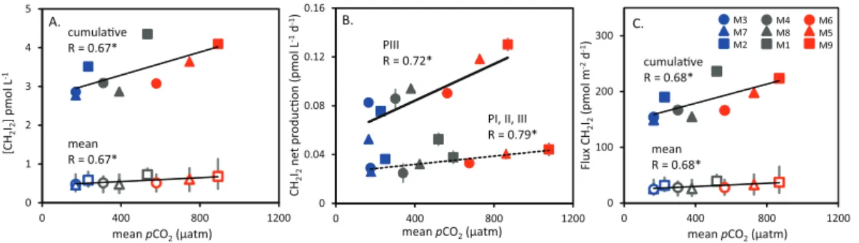
3.3 Halocarbons andpCO2

20

In order to determine the effect ofpCO₂on concentrations of halocarbons, the strength

of the correlation between mean concentrations and pCO₂ for each experimental

phase was examined. A significant increase in both mean and cumulative concen-trations of CH₂I₂under increasing CO₂was seen in PIII (R=0.67,F=5.75,p <0.05) (Fig. 4a). No further relationships were identified between the standing stocks of

halo-25

(15)

BGD

9, 8199–8239, 2012

Title Page

Tables Figures

◭ ◮

Back Close

Full Screen / Esc

Discussion

P

a

per

|

Dis

cussion

P

a

per

|

Discussion

P

a

per

|

Discussio

n

P

a

per

|

4 Discussion

Absolute concentrations of halocarbons measured in the mesocosms were compara-ble to two earlier studies that reported halocarbons from Kongsfjorden, and the data is summarised in Table 6 (Hughes, 2004; Schall and Heumann, 1993). Schall and Heumann (1993) (hereafter SH93) analysed seawater samples collected 1 km from

5

the shore during September – a comparable location to the mesocosms, during a sim-ilar season. Mean concentrations of CH₃I show strong similarity, although a greater range was observed in the mesocosms, perhaps a result of the nutrient-induced phyto-plankton growth. Concentrations of the remaining compounds were generally lower in the mesocosms than those measured by SH93. Similarly, mean concentrations were

10

consistently higher in the fjord compared to the mesocosms during this study, with the greatest difference in mean concentrations seen for CH₂I₂ (78 %) and the least diff er-ence for CH₂BrCl (28 %). Whilst differences in halocarbon concentrations between the fjord and mesocosms may be a product of the temporal progression of their respective microbial communities, variations in light regimes and exclusion of benthic processes

15

may have contributed to the variations. For instance, almost minimal ultraviolet (UV) light (<380 nm) was transmitted through the mesocosm foil (Matthias Fischer, personal communication), and furthermore, potential macroalgal sources of halocarbons were excluded from the mesocosms.

4.1 Processes controlling halocarbon concentrations in the mesocosms

20

During this experiment, 11 individual halocarbon compounds were quantified, along with numerous other biological and chemical parameters. Attempts to discuss each halocarbon individually would lead to an extensive and complicated discussion. There-fore in order to rationalise the following section, the discussion will focus on one halocarbon from each of the groups detailed in Sect. 3.2, on the assumption that

25

(16)

BGD

9, 8199–8239, 2012

Title Page

Tables Figures

◭ ◮

Back Close

Full Screen / Esc

Discussion

P

a

per

|

Dis

cussion

P

a

per

|

Discussion

P

a

per

|

Discussio

n

P

a

per

(3) CHBr₃(Br-polyhalogenated). These halocarbons are either the dominant gas from each group in terms of concentrations and/or are the most important in terms of their influence on atmospheric chemistry.

4.1.1 Iodomethane (CH3I)

The temporal dynamics of CH₃I were characterised by periods of both net loss and net

5

production, resulting in concentrations that ranged between below D.L. (<1 pmol l−1₎

and_∼10 pmol l−1_{, suggesting active turnover of this compound within the mesocosms}

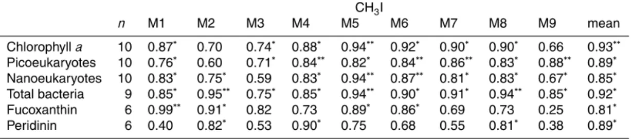
(Fig. 2a). Numerous strong relationships to biological parameters were identified, pre-dominantly during PI (Table 2). CH₃I concentrations gave significant positive correla-tions with chla, nanoeukaryotes, and phytoplankton pigment concentrations

(fucoxan-10

thin, chl C1/C2, peridinin), whilst CH₃I was inversely correlated with picoeukaryotes and total bacterial abundances. Yet, despite the apparent close association with bio-logical activity and the strong CO₂ e_ffect on a number of biological parameters (see Brussaard et al., 2012; Schulz et al., 2012; this issue), no consistent or prolonged response topCO₂was seen in the concentrations of CH₃I.

15

In order to speculate on the lack of response of CH₃I concentrations to CO₂, the processes controlling the production and removal of CH₃I in seawater must first be ex-plained. Direct biological production is thought to occur via methyl transferase enzyme activity by both phytoplankton and bacteria (Amachi et al., 2001). The strong correla-tions with a number of biological parameters in the mesocosms provide evidence for

20

this source. In addition, production is possible from the breakdown of higher molecu-lar weight iodine-containing organic matter (Fenical, 1982) and through photochemical reactions between organic matter and light (Richter and Wallace, 2004), both of which may have made some contribution to the production of CH₃I in the mesocosm. In terms of removal, CH₃I undergoes nucleophilic substitution and hydrolysis in seawater (Elliott

25

(17)

BGD

9, 8199–8239, 2012

Title Page

Tables Figures

◭ ◮

Back Close

Full Screen / Esc

Discussion

P

a

per

|

Dis

cussion

P

a

per

|

Discussion

P

a

per

|

Discussio

n

P

a

per

|

that some CH₃I undergoes consumption by bacteria, and results of laboratory incu-bations with13C-labelled CH₃I have provided evidence of significant “biological” loss rates (Hopkins, personal communication). Seawater CH₃I is also lost via the sea-to-air flux, and this comprised a relatively small component of the total loss during this experiment. For example, during PI the mean sea-to-air flux of CH₃I was estimated

5

at 73.1 pmol m−2d−1. Therefore, when scaled to allow comparison with the total net loss, assuming a 12 m deep mixed water column, this flux represents 8 fmol l−1_d−1_,

equivalent to<4 % of the total (0.25 pmol l−1_d−1_).

Clearly, the controls on seawater concentrations of CH₃I are varied and complex. Furthermore, halocarbons occur at such low levels in seawater (picomolar) that

dis-10

tinguishing the underlying processes from bulk measurements is very di_fficult. The strongest relationships between CH₃I and biological activity were seen during PI, a pe-riod when the biological response topCO₂was minimal (See Schulz et al., 2012, this issue). Over the course of PII and PIII, the coupling between CH₃I concentrations and

biological parameters such as chl a lessened, suggesting a decrease in the

impor-15

tance of direct biological production and a rise in the importance of other production processes. Consequently, a CO₂e_ffect on CH₃I of the kind seen on biological param-eters during PII and PIII was not detectable.

4.1.2 Diiodomethane (CH2I2)

The main loss pathway for CH₂I₂ in seawater is photolysis at near-ultraviolet (UV)

20

wavelengths (300–350 nm) (Martino et al., 2006). However, it is likely that this pro-cess was negligible in the mesocosms due to lack of UV transmission through the foil (Matthias Fischer, personal communication), and the solar zenith angle experienced at Ny- ˚Alesund in June (55–75◦_{) would result in little UV entering the mesocosms from}

above. The lack of photolysis may have facilitated the gradual increase in CH₂I₂

con-25

(18)

BGD

9, 8199–8239, 2012

Title Page

Tables Figures

◭ ◮

Back Close

Full Screen / Esc

Discussion

P

a

per

|

Dis

cussion

P

a

per

|

Discussion

P

a

per

|

Discussio

n

P

a

per

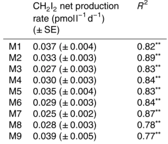
(Fig. 4a). The temporal data underwent linear regression analysis to reveal signifi-cant net production rates (pmol l−1_d−1_{) in all mesocosms (Table 3). Rates ranged from}

0.027 pmol l−1_d−1_{in M3 to 0.039 pmol l}−1_d−1_{in M9. Next, net production rates for each}

mesocosm underwent correlative analysis with the associated meanpCO₂, revealing significant positive correlations for both the whole experiment (dashed line symbols,

5

R=0.79,p <0.05) and for PIII (solid line,R=0.72,p <0.05) (Fig. 4b).

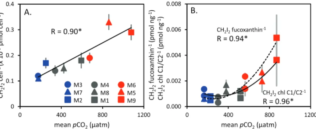
Furthermore, concentrations of CH₂I₂ were strongly, and often significantly, corre-lated with a number of biological parameters. Shown in Table 4, CH₂I₂ was closely correlated with both chlaand total bacteria for the whole experiment, whilst close re-lationships with the phytoplankton pigments fucoxanthin and peridinin were observed

10

during PIII. The ratios of CH₂I₂ to a number of biological parameters were found to be strongly correlated with pCO₂ (Fig. 5). The ratio of CH₂I₂ to bacteria cell num-bers (×10−9pmol cell−1) significantly increased with increasing CO2 for the entire

ex-periment (Fig. 5a) whilst ratios of CH₂I₂ to the phytoplankton pigments (pmol ng−1, fucoxanthin and chl C1/C2) showed similarly strong and significant trends during PIII

15

(Fig. 5b, c). In summary, strong relationships between CH₂I₂and the biological commu-nities of the mesocosms were observed, in particular with total bacterial abundances. In addition, there appeared to be an increase in net production of CH₂I₂in response to increasingpCO₂. The possible reasons for this will be explored in the following section. The production of I-polyhalocarbons (CH₂I₂, CH₂ClI) can be the result of

iodoper-20

oxidase enzyme activity that catalyses the destruction of H₂O₂and stimulates iodina-tion reaciodina-tions to form polyhalogenated products (Moore et al., 1996; Leblanc et al., 2006). The exact reason for algal-mediated production of volatile halocarbons is not fully understood, although theories exist as to the function of this process (Manley, 2002; Leblanc et al., 2006). As the consequence of haloperoxidase activity is to reduce

25

(19)

BGD

9, 8199–8239, 2012

Title Page

Tables Figures

◭ ◮

Back Close

Full Screen / Esc

Discussion

P

a

per

|

Dis

cussion

P

a

per

|

Discussion

P

a

per

|

Discussio

n

P

a

per

|

The strong significant negative correlations between CH₂I₂and total bacterial abun-dances over the duration of the experiment are intriguing and suggest some bacterial involvement in the turnover of this compound. There are no reported studies of the biological consumption of CH₂I₂. However, there is direct evidence for bacterial con-sumption of CH₂Br₂ (Goodwin et al., 1997, 1998), so this process cannot be ruled out

5

for CH₂I₂. A small number of studies have investigated the involvement of bacteria in the production of I-polyhalocarbons, yielding somewhat limited and speculative infor-mation. Strains of iodine-oxidising bacteria (IOB) have been isolated from seawater, im-plicating species closely related to the marine bacteriumRoseovarius tolerans(aerobic bacteriochlorophylla-producer) (Fuse et al., 2003; Amachi et al., 2008). During

labo-10

ratory enrichment incubations, IOB directly produced free iodine (I₂) which led to the production of abundant organic iodine species, specifically CH₂I₂, CH₂ClI and CHI₃, via an extracellular oxidase enzyme. Although enrichment incubations are far removed from processes occurring in natural seawater, Amachi (2008) speculates that IOB may be widely distributed in the marine environment, raising the possibility that given the

15

right conditions, IOB could significantly contribute to the production of CH₂I₂in the ma-rine environment. The significant negative correlations between bacterial abundance and CH₂I₂ concentration as well as increasing ratios of CH₂I₂ per bacteria cell with increasingpCO₂ suggest either: (1) an increase in bacterial production of CH₂I₂, or (2) a decrease in bacterial consumption of CH₂I₂, in response to increasingpCO₂.

20

Due to its high reactivity and short photolytic lifetime, CH₂I₂ is potentially one of the most important sources of iodine atoms to the coastal marine boundary layer (Carpenter et al., 1999). Thus, changes to the sea-to-air flux of this compound could have implications for the catalytic destruction of tropospheric ozone (Chameides and Davis, 1980) and for new particle formation (O’Dowd et al., 2002). Mean fluxes ranged

25

from−0.02 (M6) to 4.1 pmol m−2d−1 (M4) during PI (overall mean 1.06 pmol m−2d−1), and 7.1 (M6) to 34.4 pmol m−2_d−1 _{(M1) in PII (overall mean 12.3 pmol m}−2_d−1_).

(20)

BGD

9, 8199–8239, 2012

Title Page

Tables Figures

◭ ◮

Back Close

Full Screen / Esc

Discussion

P

a

per

|

Dis

cussion

P

a

per

|

Discussion

P

a

per

|

Discussio

n

P

a

per

a number of weaknesses in the calculation of the flux – not least the atmospheric values (Schall and Heumann, 1993), so conclusions should be drawn with caution. In PI and PII, no significant di_fferences in flux were detected between mesocosms. Fig-ure 4c shows the estimated mean cumulative fluxes for PIII plotted as a function of pCO₂, showing a significant relationship (p=0.04) with increasingpCO₂.

5

4.1.3 Bromoform (CHBr3)

CHBr₃ is the most abundant form of volatile organic bromine in seawater (Carpenter and Liss, 2000; Quack et al., 2007; Hughes et al., 2009), and predictably dominated the concentrations of bromocarbons in the mesocosms (Fig. 2f–j). No relationship between CHBr₃concentrations andpCO₂treatment was observed, and there was a high degree

10

of similarity in concentrations in the majority of mesocosms.

A key feature of the CHBr₃ data were the consistently higher concentrations ob-served in M1, most apparent fromt₁₂ tot₁₉, and fromt₂₀ tot₂₇ (Fig. 2f). The elevated concentrations occurred immediately after a period of rapid net production in all meso-cosms. Significant net production rates were detected in M1 for the periods t₁₀–t₁₃

15

(22.3±4.1 pmol d−1,p=0.03) andt19–t21 (33.0±1.9 pmol d−1,p=0.04), significantly

higher than the net production rates of the remaining mesocosms. These periods of net production were immediately followed by net loss overt₁₃–t₁₆, andt₂₁–t₂₇ in all meso-cosms, during which M1 displayed the greatest rates of net loss (12.6±1.8 pmol d−1, p=0.02 and 8.0±1.0 pmol d−1,p=0.001, respectively). This suggests enhanced

pro-20

duction and turnover of CHBr₃in M1 relative to the other mesocosms.

During the final phase of the experiment significant net loss rates were observed in all mesocosms, ranging from the maximum in M1 (see above) to a minimum of 2.9_±0.3 pmol d−1_{in M8 over}_t

21–t27(Table 5). There was found to be a no relationship

between the net loss rates andpCO₂ for this period of the experiment (Fig. 6a). This

25

(21)

BGD

9, 8199–8239, 2012

Title Page

Tables Figures

◭ ◮

Back Close

Full Screen / Esc

Discussion

P

a

per

|

Dis

cussion

P

a

per

|

Discussion

P

a

per

|

Discussio

n

P

a

per

|

the possibility of an effect ofpCO₂, the potential mechanisms responsible for the diff er-ences in net production and loss of CHBr₃between the mesocosms were investigated further. In seawater, a number of processes act as sinks for CHBr₃including (i) hydrol-ysis, (ii) reductive dehalogenation, (iii) halogen substitution, and (iv) photolysis. With half-lives at Arctic seawater temperatures of 680–1000 yr and 74 yr, respectively, (i)

5

and (iii) are of little importance in this discussion (Quack and Wallace, 2003). Reduc-tive dehalogenation (ii) can occur in anaerobic conditions so is also not relevant to the mesocosms (Quack and Wallace, 2003; Vogel et al., 1987). Microbial degradation has not been directly observed (Goodwin et al., 1997), although there is some evidence that it may occur at reasonable rates within the water column of both polar and

trop-10

ical waters (Hughes et al., 2009; Quack et al., 2007). Photolysis is considered to be the largest internal sink for CHBr₃(Carpenter and Liss, 2000); however this constitutes only∼2 % of the sea-to-air flux. The mean estimated flux of CHBr3for all mesocosms,

when scaled as described for CH₃I, was 0.30 pmol l−1_d−1_{(min. 0.26 pmol l}−1_d−1_(M8),

max. 0.36 pmol l−1d−1 (M1)), with little difference between mesocosms, and no effect

15

ofpCO₂. Therefore, these estimated fluxes can explain between 5 % and 12 % of the net loss.

Using this information it is possible to speculate on the dominant processes control-ling the concentration of CHBr₃ in the mesocosms. A key feature of the CHBr₃ data was a strong and significant relationship between the observed net loss rates

(cor-20

rected for the sea-to-air flux) over t₂₁–t₂₇ and the seawater concentrations of CHBr₃ on t21 (Fig. 6b). This apparent concentration-dependence of loss rates may indicate

that the turnover of CHBr₃ in the mesocosms is related to biological processes, with the linear relationship representing the biological uptake rate kinetics. This is supported by the observed significant relationships between CHBr₃concentrations and total

bac-25

teria abundances (Table 5).

(22)

BGD

9, 8199–8239, 2012

Title Page

Tables Figures

◭ ◮

Back Close

Full Screen / Esc

Discussion

P

a

per

|

Dis

cussion

P

a

per

|

Discussion

P

a

per

|

Discussio

n

P

a

per

et al., 2012, this issue). A similar affect can be seen over the period t₁₉–t₂₁. Net production rates of CHBr₃ ranged from 0.6 pmol l−1_d−1_{(M3) to 33.0 pmol l}−1_d−1 _in

M1, with those in M1 significantly higher. Again, the higher net production rates of CHBr₃ in M1 were concomitant with significantly lower bacterial biomass production on botht₂₀ (M1₌23.62 ng C l−1_h−1_{, mean of all mesocosms}

=87.16 ng C l−1_h−1_{) and} 5

t₂₂ (M1=75.97 ng C l−1h−1, mean of all mesocosms=169.52 ng C l−1h−1). Lower bac-terial biomass production may be indicative of a decrease in bacbac-terial activity, leading to lower consumption rates and higher net production rates of CHBr₃. These di_ff er-ences may have contributed to the range of concentrations of CHBr₃measured ont₂₁. Similar patterns can be seen in the CH₂Br₂and CH₂BrCl data (detail not shown here),

10

confirming similar production and consumption pathways of these polybromocarbons, but apparently unaffected by the alteredpCO₂conditions.

4.2 Comparison to a previous mesocosm experiment

Concentrations of a variety of halocarbons from a CO₂ enrichment experiment

per-formed in temperate, coastal waters o_ff Bergen, Norway in 2006 were reported by

15

Hopkins et al. (2010). During the 2006 experiment, maximum chla concentrations of 6–11 µg l−1 _{were more than double of those measured in this study, and the}

plank-ton community showed a strong response to CO₂, with significant decreases in chla and microbial plankton under high CO₂. Nevertheless, both the concentrations and the general response of the bromocarbons to biological activity andpCO₂ showed some

20

similarity to the present study conducted in Arctic waters. In contrast, concentrations of iodocarbons were markedly higher during the 2006 experiment, particularly for CH₂I₂ and CH₂ClI with maximum concentrations of ∼700 and ∼600 pmol l−1, respectively. Furthermore, large, and in some cases significant, reductions in concentrations of all iodocarbons occurred at higher pCO₂ (CH₃I: ₋44 %, C₂H₅I: ₋35 %, CH₂I₂: ₋27 %,

25

(23)

BGD

9, 8199–8239, 2012

Title Page

Tables Figures

◭ ◮

Back Close

Full Screen / Esc

Discussion

P

a

per

|

Dis

cussion

P

a

per

|

Discussion

P

a

per

|

Discussio

n

P

a

per

|

activity observed in this Arctic experiment may have suppressed a clear response in the iodocarbon concentrations to increasing CO₂of the kind seen in the 2006 experiment.

5 Conclusions

Concentrations of a range of halocarbons were measured during a 5-week CO₂

-perturbation mesocosm experiment in Kongsfjorden, Spitsbergen, during June and July

5

2010. The temporal standing stocks of the majority of halocarbons did not significantly

respond topCO₂ over a range from ∼175 µatm to∼1085 µatm. Halocarbon

concen-trations did show a large number of significant correlations with a range of biological parameters suggesting some influence of the biological communities on the produc-tion and consumpproduc-tion of these trace gases in Arctic waters. The temporal dynamics

10

of CH₃I, combined with strong correlations with biological parameters, indicated a bio-logical control on concentrations of this gas. However, despite a CO₂e_ffect on various components of the community, no effect ofpCO₂was seen on CH₃I. CH₂I₂ concentra-tions were closely related to chlaand total bacteria over the whole experiment and with the phytoplankton pigments fucoxanthin and peridinin during PIII, strongly suggesting

15

biological production of this gas. Both the concentrations and the net production of CH₂I₂ showed some sensitivity topCO₂, with a significant increase in net production rate and sea-to-air flux at higherpCO₂, particularly during the later stages of the ex-periment. The temporal dynamics of CHBr₃ indicated rapid turnover of this gas, and concentrations varied between mesocosms, although not explainable bypCO₂

treat-20

ment. Instead, net loss rates (corrected for loss via gas exchange) displayed a degree of concentration-dependence, and strong negative correlations with bacteria during pe-riods of net loss suggest a degree of bacterial consumption of CHBr₃in Arctic waters. The results of the first Arctic OA mesocosm experiment provide invaluable information on the production and cycling of halocarbons in Arctic waters, demonstrating strong

25

(24)

BGD

9, 8199–8239, 2012

Title Page

Tables Figures

◭ ◮

Back Close

Full Screen / Esc

Discussion

P

a

per

|

Dis

cussion

P

a

per

|

Discussion

P

a

per

|

Discussio

n

P

a

per

The role of halocarbons in Arctic atmospheric chemistry may increase in importance in the coming decades due to increases in open water and productivity with the loss of sea ice (Mahajan et al., 2010; Kahru et al., 2011; Stroeve et al., 2011); this work enhances our understanding of the marine production and cycling of halocarbons in a region set to experience rapid environmental change.

5

Acknowledgements. This work is a contribution to the European Project on OCean

Acidifica-tion (EPOCA) which received funding from the European Community’s Seventh Framework Programme (FP7/2007–2013) under grant agreement no. 211384. We gratefully acknowledge the logistical support of Greenpeace International for its assistance with the transport of the

mesocosm facility from Kiel to Ny- ˚Alesund and back to Kiel. We also thank the captains and

10

crews of M/V ESPERANZA of Greenpeace and R/V Viking Explorer of the University Centre in Svalbard (UNIS) for assistance during mesocosm transport and during deployment and re-covery in Kongsfjorden. We thank Signe Koch Klavsen for providing phytoplankton pigment data and Matthias Fischer for UV measurements through the mesocosm foil. We are grateful to the UK Natural Environmental Research Council for the accommodation and support provided

15

through the NERC-BAS station in Ny- ˚Alesund. We also thank the staffof the French-German

Arctic Research Base at Ny- ˚Alesund, in particular Marcus Schuhmacher, for on-site logistical

support. Financial support was provided through the European Centre for Arctic Environmental Research (ARCFAC) (grant number ARCFAC026129-2009-140) and through Transnational Ac-cess funds by the EU project MESOAQUA under grant agreement no. 22822. Finally, we would

20

like to thank Ulf Riebesell, Sebastian Krug and the whole of the Svalbard mesocosm team, who showed great team spirit and comradeship and helped to make the experiment both enjoyable and successful.

References

Amachi, S.: Microbial contribution to global iodine cycling: volatilization, accumulation,

redcu-25

tion, oxidation and sorption of iodine, Microbes Environ., 23 (4), 269–276, 2008.

(25)

BGD

9, 8199–8239, 2012

Title Page

Tables Figures

◭ ◮

Back Close

Full Screen / Esc

Discussion

P

a

per

|

Dis

cussion

P

a

per

|

Discussion

P

a

per

|

Discussio

n

P

a

per

|

Calvert, J. G. and Lindberg, S. E.: Potential influence of iodine-containing compounds on the chemistry of the troposphere in the polar spring. I. Ozone depletion, Atmos. Environ., 38, 5087–5104, 2004a.

Carpenter, L. J. and Liss, P. S.: On temperature sources of bromoform and other reactive or-ganic bromine gases, J. Geophys. Res., 105 (D16), 20539–20547, 2000.

5

Carpenter, L. J., Sturges, W. G., Penkett, S. A., Liss, P. S., Alicke, B., Hebestreit, K., and Platt, U.: Short lived alkyl iodides and bromides at Mace Head, Ireland: links to biogenic sources and halogen oxide production, J. Geophys. Res., 104, 1679–1689, 1999.

Chameides, W. L. and Davis, D. D.: Iodine: its possible role in tropospheric photochemistry, J. Geophys. Res.-Atmos., 85, 7383–7398, 1980.

10

Davis, D., Crawford, J., Liu, S., McKeen, S., Bandy, A., Thornton, D., Rowland, F., and Blake, D.: Potential impact of iodine on tropospheric levels of ozone and other critical oxidants, J. Geo-phys. Res., 101, 2135–2147, 1996.

DeBruyn, W. J. and Saltzman, E. S.: Diffusivity of methyl bromide in water, Mar. Chem., 56,

51–57, 1997.

15

Elliott, S. and Rowland, F. S.: Nucleophilic substitution rates and solubilities for methyl halides in seawater, Geophys. Res. Lett., 20, 1043–1046, 1993.

Fenical, W.: Natural products chemistry in the marine environment, Science, 215, 923–928, 1982.

Fuse, H., Inoue, H., Murakami, K., Takimura, O., and Yamaoka, Y.: Production of free and

20

organic iodine byRoseovariusspp., FEMS Microbiol. Lett., 229, 189–194, 2003.

Goodwin, K. D., Lidstrom, M. E., and Oremland, R. S.: Marine bacterial degradated of bromi-nated methanes, Environ. Sci. Technol., 31, 3188–3192, 1997.

Goodwin, K. D., Schaefer, J. K., and Oremland, R. S.: Bacterial oxididation of dibromomethane and methyl bromide in natural waters and enrichment cultures, Appl. Environ. Microb., 64,

25

4629–4636, 1998.

Goodwin, K. D., Varner, R. K., Crill, P. M., and Oremland, R. S.: Consumption of tropospheric levels of methyl bromide by C-1 compound-utilizing bacteria and comparison to saturation kinetics, Appl. Environ. Microb., 67, 5437–5443, 2001.

Happell, J. D. and Wallace, D. W. R.: Methyl iodide in the Greenland/Norwegian Seas and

30