Submitted14 June 2016
Accepted 23 July 2016
Published7 September 2016
Corresponding author
A. Townsend Peterson, town@ku.edu
Academic editor
Mark Costello
Additional Information and Declarations can be found on page 16
DOI10.7717/peerj.2362
Copyright
2016 Peterson et al.
Distributed under
Creative Commons CC-BY 4.0 OPEN ACCESS
Digital Accessible Knowledge and
well-inventoried sites for birds in Mexico:
baseline sites for measuring faunistic
change
A. Townsend Peterson1, Adolfo G. Navarro-Sigüenza2and Enrique Martínez-Meyer3
1Biodiversity Institute, University of Kansas, Lawrence, KS, United States
2Museo de Zoología, Facultad de Ciencias, Universidad Nacional Autónoma de México, México,
Distrito Federal, México
3Instituto de Biología, Universidad Nacional Autónoma de México, México, Distrito Federal, México
ABSTRACT
Background. Faunal change is a basic and fundamental element in ecology, biogeography, and conservation biology, yet vanishingly few detailed studies have documented such changes rigorously over decadal time scales. This study responds to that gap in knowledge, providing a detailed analysis of Digital Accessible Knowledge of the birds of Mexico, designed to marshal DAK to identify sites that were sampled and inventoried rigorously prior to the beginning of major global climate change (1980).
Methods. We accumulated DAK records for Mexican birds from all relevant online biodiversity data portals. After extensive cleaning steps, we calculated completeness indices for each 0.05◦pixel across the country; we also detected ‘hotspots’ of
sam-pling, and calculated completeness indices for these broader areas as well. Sites were designated as well-sampled if they had completeness indices above 80% and >200 as-sociated DAK records.
Results. We identified 100 individual pixels and 20 broader ‘hotspots’ of sampling that were demonstrably well-inventoried prior to 1980. These sites are catalogued and documented to promote and enable resurvey efforts that can document events of avi-faunal change (and non-change) across the country on decadal time scales.
Conclusions. Development of repeated surveys for many sites across Mexico, and particularly for sites for which historical surveys document their avifaunas prior to major climate change processes, would pay rich rewards in information about distri-butional dynamics of Mexican birds.
SubjectsBiodiversity, Biogeography, Conservation Biology, Zoology
Keywords Biodiversity, Biodiversity change, Faunal dynamics, Historical surveys, Resurveys
INTRODUCTION
how community composition changes as a result are key in determining essentially all results in these areas of ecology and evolutionary biology. Although biogeographers invest fundamentally in retracing the geography of evolving lineages over long periods of time, strangely little information exists on short-term dynamics of species’ distributions and community composition (e.g.,Nunes et al., 2007;Tingley & Beissinger, 2009).
An important opportunity to understand these shorter-term dynamics of distributions and communities by means of longitudinal comparisons of inventories of local faunas and floras. That is, when a baseline of solid, complete, and well-documented knowledge exists about a site (Colwell & Coddington, 1994;Peterson & Slade, 1998;Soberón & Llorente, 1993), re-surveys over years, decades, and centuries can offer a fascinating view into the natural dynamics of species’ ranges and the effects of human presence and activities. Drivers of these changes may act both on local scales (e.g., effects of land use change) and on global scales (e.g., effects of climate change), and potentially may interact as well; studies integrating and comparing effects of different such drivers are particularly rare (e.g.,Peterson et al., 2015;Rubidge et al., 2011). Of course, detailed documentation of species identifications and of the completeness of inventory efforts are necessary for both the baseline and the resurvey, but the general paradigm has considerable potential.
Previous baseline/re-survey efforts have yielded fascinating information about faunas and floras. For example,Nilsson, Franzén & Jönsson (2008)documented 40% extirpation of butterfly species over a 90+ year span on a plot in southern Sweden, and found that species disappearing from the fauna tended to be those with a short flight length period, narrow habitat breadth, and small distributional area in Europe; however, only flight length period was significant in multivariate analyses.Grixti & Packer (2006)studied bee communities at a site in southern Ontario, and documented community changes and diversity increases over a 40+ year span, likely in response to successional changes in the surrounding landscapes.Scholes & Biggs (2005)proposed a biodiversity intactness index, and showed widespread population declines, particularly among mammals, and ecosystem declines concentrated in grasslands, across a large region of southern Africa. In California, important efforts have been carried out to resurvey sites studied by Joseph Grinnell a century ago, detecting fascinating distributional (Tingley & Beissinger, 2009), phenotypic (Leache, Helmer & Moritz, 2010), and genetic (Rubidge et al., 2011) changes in vertebrate species and communities (Moritz et al., 2008).
Curiously, however, to our knowledge at least, this short list includes all sites that have seen baseline and re-survey inventories of birds in the country, such that the nature and pattern of avifaunal change across Mexico remains very poorly characterized.
The purpose of this paper is to stimulate and enable a next generation of such re-survey efforts for birds across Mexico by means of cataloguing sites for which solid documentation exists for the original baseline inventory, and for which the baseline inventory is demonstrably complete. We reviewed all existing Digital Accessible Knowledge (DAK;Sousa-Baena, Garcia & Peterson, 2013) regarding the birds of Mexico: we probed four major online data portals for relevant data (i.e., bird records from Mexico prior to 1980), and evaluated inventory completeness at two spatial extents (0.05◦ grid squares,
and coarser hotspots of sampling). We present a simple list and catalog of sites that have seen relatively complete (i.e.,≥80% of avifauna known and documented) inventories, as
a challenge and stimulus to the ornithological community in Mexico. Resurvey of these localities would provide rich and informative rewards in understanding the dynamics of bird populations and distributions across the country.
MATERIALS & METHODS
This analysis is based on a suite of assumptions about data quality and appropriate resolutions inherent in biodiversity data. For instance, we used single days as the unit of sampling effort throughout our analyses, as this resolution has proven an effective balance between too much and too little resolution; temporal information finer than the level of day is rarely available with older biodiversity data, whereas coarse temporal resolution can underappreciate the efficacy of short-term, intensive inventory efforts. Hence, a basic working data set was the combination of species identification, day (i.e., unique combinations of year, month, and day), and place. This latter we defined in various ways, described below, but we note that we used both geographic coordinates and textual locality descriptions to avoid loss of information owing to lack of georeferencing, at least to every extent possible.
Data sources and quantities
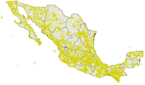
Figure 1 Digital accessible knowledge of bird distributions (481,409 unique combinations of species
×place×time) across Mexico prior to 1980, drawn from GBIF, VertNet, REMIB, and UNIBIO
(records are not coded by source owing to frequent overlaps among sources in serving copies of the same record).
Table 1 Summary of initial data downloaded from each of four biodiversity data portals for Mexican vertebrate classes, and the relative redundancy of records in each, at the level of species×time (year, month, day)×place (geographic coordinates, textual descriptions).Note that subsequent data cleaning steps changed these initial tallies of redundancy, as they sought synonymies for taxon and place that may not have been visible in this initial step.
GBIF VertNet REMIB UNIBIO
Raw records 2,426,732 299,280 584,569 29,348
Unique records 1,917,800 226,004 431,240 23,446
Percent reduction 21.0 24.5 26.2 20.1
Data reduction and cleaning
Initial data downloads totaled tens to hundreds of thousands of records from Mexico from each of the data portals, reaching millions from GBIF (although the GBIF numbers are largely from eBird and aVerAves, which come in greatest part from post-1980;Fig. 1,Table 1). We expected considerable redundancy between data sources, in the form of situations in which the same species was collected or recorded at the same place on the same day, so we embarked on a lengthy process of data reduction and cleaning. Without a doubt, some mistakes were made, and some information was lost, but this effort aimed to detect and highlight the major features of Mexican bird DAK, rather than all of the details. That is, we focused on sites that had the most information available, and explicitly excluded information for less-well-known sites.
order, family, genus, and species, to permit identification of the most difficult names), date collected (year, month, and day), and place (latitude and longitude, when available, and state, municipality, and specific locality). We filtered these records to remove all those records from years after 1980. The initial total of 2,598,478 records distilled to 845,658 (a 67.5% reduction) that both (1) had dates and (2) were not from after 1980.
From this set, we extracted 10,762 unique combinations of order, family, genus, and species, which included diverse name combinations, and required considerable work to distill to a consistent suite of names corresponding to the birds of Mexico. We avoided the temptation to attempt to take the taxonomic treatment to a newer authority list (e.g.,Gill & Donsker, 2014;Navarro-Sigüenza & Peterson, 2004;Peterson & Navarro-Sigüenza, 2006) because taxonomic splitting, which has dominated recent years of taxonomic work, would cause considerable confusion of names applied to older records. Hence, we reduced the initial, highly redundant set of names to 1,027 names that coincided with the taxonomy of the American Ornithologists’ Union (AOU, 1998), except that we mergedEmpidonax traillii andE. alnorum, in light of very frequent confusion in identification (Heller et al., 2016). This step was achieved based on long years of experience with Mexican bird taxonomy, plus occasional consultation of the literature (Monroe & Sibley, 1993;Peters, 1931–1987) and online (http://avibase.bsc-eoc.org/) resources.
A second step was to summarize date information as a concatenation of year, month, and day (e.g., 1964_7_16). Records with dates for which all three time elements were missing were removed from analysis, but records with partial dates (e.g., year and month, but not day) were treated as a unique time event. All data management was carried out in OpenRefine (http://openrefine.org), which permitted many important initial steps of combining similar names, and in Microsoft Access, which permitted development of customized queries for further refinement.
Data analysis
Perhaps the most difficult-to-manage of the fields was that of ‘place.’ Here, we used a three-step process that aimed to retain a maximum of locality information, yet avoid the massive and prohibitive task of full georeferencing of all records for which no geographic coordinates were available. Hence, (1) we used the 502,935 records that had latitude-longitude data in a first-pass analysis that aimed to identify single sites that were well inventoried, and to identify somewhat broader ‘hotspots’ of sampling (details provided below). Next (2), we used locality names associated with the records falling in the hotspots to probe the data lacking georeferences, and thereby rescued >54,000 records. Finally (3), we inspected the remaining data records—those lacking georeferences—to identify additional sites that merited analysis (five such additional, un-georeferenced sites indeed proved to be relatively well-inventoried, such that this step was important; see below). In this way, the number of localities that needed to be georeferenced was minimized, and yet we managed to include the great bulk of Mexican DAK in our analyses.
of sampling that may or may not prove to be well-inventoried. We first filtered this data set to retain only the records that were within 0.05◦(5–6 km) of the administrative outline
of Mexico—this step left 499,794 (99.4%) records for initial analysis. This initial data set was further reduced to 481,409 (95.7%) that came from 1980 or before.
We then created a shapefile with square elements of 0.05◦for Mexico, and eliminated
pixels that were >0.05◦ from the administrative boundaries of Mexico. We then used
a spatial join to count numbers of records in each polygon; numbers of records per cell ranged from nil to as high as 15,464 (a pixel centered on Chilpancingo, Guerrero). We used optimized hot spot analysis (implemented in ArcGIS, version 10.2) to identify concentrations of sampling effort across the country—we used the Getis-Ord Gi* statistic (Hot Spot Analysis tool), and focused only on hotspots (0.05◦grid squares) significant at
the highest (99%) confidence level. We isolated these well-sampled suites of pixels as a separate shapefile, and then merged pixels in contiguous sets as preliminary hypotheses of broader hotspots of sampling, which we enriched with more records in step 2 (see below). We also used the initial data set to develop an identification of single 0.05◦pixels that
were well-inventoried, as follows. The 481,409 pre-1980 records remaining after clipping to the country boundaries reduced to 277,249 (57.6%) unique combinations of species
×date×pixel. We calculatedSobsas the number of species that have been recorded from each pixel,N as the total number of unique combinations of species×date from each pixel
(and thus we set a base spatial resolution as that of the 0.05◦grid, such that co-occurrences
of species within these pixels are assumed to be sympatric), andaandbas the numbers of species recorded exactly once and exactly twice, respectively, from each pixel. We then used these data to calculate, for each pixel, the Chao2 estimator of expected species richness, with its associated adjustment for small sample sizes (Colwell, 1994–present), as
Sexp=Sobs+
N−1
N
a(a−1)
2(b+1)
. (1)
Completeness was then calculated asC=Sobs/Sexp. To avoid including occasional localities
with small sample sizes and artificially ‘complete’ inventories, we further removed all pixels for whichN<200. We summarized these calculations in a table, which we then imported
into ArcGIS and joined to the grid shapefile for visualization.
values were then recalculated for each hotspot just as they were calculated in Step 1 for each pixel.
Step 3: This final step involved review of the remaining non-georeferenced records, even after the rescue of Step 2. That is, Step 2 focused on non-georeferenced records that corresponded to already-identified pixels and hotspots, and that could be used to enrich the existing (georeferenced) data from those sites. This third step, however, involved a look at the remaining data to see if additional well-known sites could be identified.
We assembled the raw locality descriptors, and tallied numbers of records associated with each; we did some minor cleaning and synonymizing of minor variants on locality descriptors to maximize numbers of records for each locality. Finally, we developed completeness indices (as described above) for each of the non-georeferenced localities that had a raw sample size (i.e., unique combinations of locality descriptor, year/month/day, and species) of≥200 records. Because the focus of these exercises is on detecting the
few well-inventoried sites, rather than characterizing the overall sampling landscape, no biases are introduced by this rescue step. All localities meeting an arbitrary criterion of completeness,C≥0.8, were then georeferenced and included among well-known sites.
Data availability
All data managed in this study are openly available, or will be shortly, as institutional permissions are finalized, from GBIF (http://www.gbif.org), VertNet (http://www. vertnet.org/), REMIB (http://www.conabio.gob.mx/remib/doctos/remib_esp.html), and UNIBIO (http://unibio.unam.mx/). A full synonymy of locality names in relation to the hotspots identified in this paper is available at http://hdl.handle.net/1808/20674. GIS shapefiles showing the two sets of hotspots identified in this paper are available at http://hdl.handle.net/1808/20673.
RESULTS
Processing data available for birds of Mexico from raw DAK downloads into usable records of species at localities on particular days involved considerable reduction in numbers of records (Table 1). Simply progressing from raw to unique combinations of species×locality ×geographic coordinates×year×month×day involved a reduction of 20.1–26.2%
in numbers of records (note that this reduction step was done prior to removing records post-1980). Subsequent data cleaning and reduction steps (see Methods, above) reduced redundancy both among data sources (GBIF, VertNet, REMIB, UNIBIO) and among nearby localities, leaving a final number of 481,409 records for analysis.
A first analysis focused on 277,249 unique combinations of species×date collected ×0.05◦pixel. These records fell in pixels in numbers ranging from nil to 15,464 records
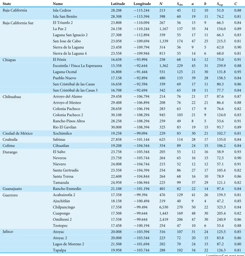
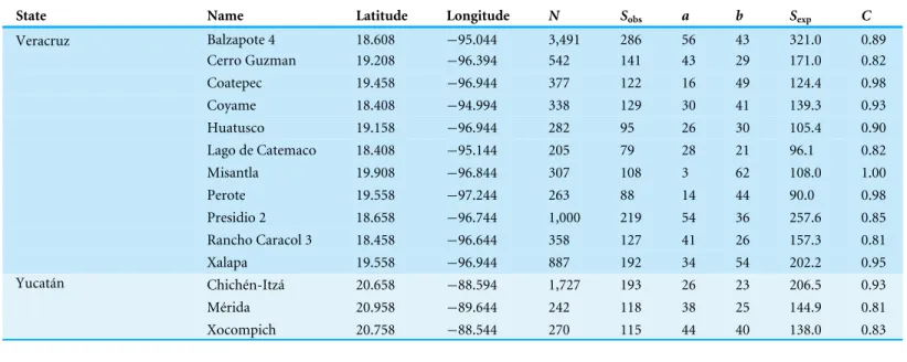
(Chilpancingo, Guerrero). Processing records in each pixel into estimates of expected numbers of species and estimated inventory completeness (Table 2;Fig. 2), we found that 24 pixels were complete at the level ofC≥0.9, and a further 71 pixels were complete at
the level ofC≥0.8. The well-inventoried sites were well-distributed across the country,
Table 2 Summary of individual 0.05◦grid squares that are well inventoried (C≥0.8) across Mexico.Names of grid squares refer to the shapefile
dataset summarizing the geographic distribution of these sites.
State Name Latitude Longitude N Sobs a b Sexp C
Isla Cedros 28.208 −115.244 213 45 12 10 51.0 0.88
Baja California
Isla San Benito 28.308 −115.594 398 60 19 11 74.2 0.81
El Triunfo 2 23.808 −110.094 267 56 15 9 66.5 0.84
La Paz 2 24.158 −110.244 1,167 137 35 34 154.0 0.89
Laguna San Ignacio 2 27.308 −112.894 339 55 17 11 66.3 0.83
San Jose de Cabo 23.058 −109.694 1,339 174 47 25 215.5 0.81
Sierra de la Laguna 23.458 −109.794 314 56 9 5 62.0 0.90
Baja California Sur
Sierra de la Laguna 4 23.558 −109.944 813 55 14 6 68.0 0.81
El Fénix 16.658 −93.994 258 68 14 12 75.0 0.91
Escuintla / Finca La Esperanza 15.358 −92.644 1,362 229 45 31 259.9 0.88
Laguna Ocotal 16.808 −91.444 531 125 21 30 131.8 0.95
Pueblo Nuevo 17.158 −92.894 480 133 39 28 158.5 0.84
San Cristóbal de las Casas 16.658 −92.594 339 69 17 11 80.3 0.86
Chiapas
San Cristóbal de las Casas 3 16.708 −92.694 342 65 18 11 77.7 0.84
Arroyo del Alamo 29.458 −106.794 214 76 21 17 87.6 0.87
Arroyo el Mesteo 29.408 −106.894 208 76 22 21 86.4 0.88
Colonia Pacheco 28.658 −106.194 283 63 17 9 76.6 0.82
Colonia Pacheco 2 30.108 −108.294 945 103 21 9 124.0 0.83
Rancho Pinos Altos 28.258 −108.294 259 49 8 5 53.6 0.91
Chihuahua
Rio El Gavilan 30.008 −108.394 325 83 19 15 93.7 0.89
Ciudad de México Xochimilco 19.258 −99.094 229 83 30 21 102.7 0.81
Coahuila Sabinas 27.858 −101.144 625 114 28 17 135.0 0.84
Colima Cihuatlan 19.208 −104.544 354 89 24 15 106.2 0.84
El Salto 23.758 −105.544 205 55 12 16 58.9 0.93
Neveros 23.758 −105.744 264 65 16 15 72.5 0.90
Nievero 24.008 −104.744 215 52 12 12 57.1 0.91
Santa Gertrudis 23.558 −104.394 254 86 27 17 105.4 0.82
Santa Teresa 22.608 −104.844 264 68 16 10 78.9 0.86
Durango
Tamazula 24.958 −106.944 225 99 37 29 121.1 0.82
Guanajuato Rancho Enmedio 21.108 −101.194 401 82 22 14 97.4 0.84
Acahuizotla 2 17.358 −99.394 476 129 41 26 159.3 0.81
Ajuchitlán 18.158 −100.494 219 40 9 4 47.2 0.85
Chilpancingo 17.558 −99.494 6,530 270 50 22 323.3 0.84
Cuapongo 17.508 −99.644 1,443 169 48 30 205.4 0.82
Omiltemi 2 17.558 −99.644 2,419 206 47 30 240.9 0.86
Guerrero
Teotepec 17.458 −100.194 254 47 10 6 53.4 0.88
Atoyac 20.008 −103.594 316 107 31 24 125.5 0.85
Atoyac 2 20.008 −103.544 223 72 20 15 83.8 0.86
Lagos de Moreno 2 21.508 −101.694 202 70 24 15 87.2 0.80
Jalisco
Tapalpa 19.958 −103.744 288 102 34 22 126.3 0.81
Table 2(continued)
State Name Latitude Longitude N Sobs a b Sexp C
Apatzingan 19.158 −102.444 244 68 18 12 79.7 0.85
Pátzcuaro 19.458 −101.594 361 111 35 23 135.7 0.82
Rancho El Bonete 18.958 −101.894 297 95 30 20 115.6 0.82
Tzitzio 19.608 −100.944 285 78 19 13 90.2 0.87
Tzitzio 2 19.658 −100.894 299 97 32 22 118.5 0.82
Uruapan 19.408 −101.994 391 94 26 14 115.6 0.81
Michoacán
Zacapu 19.808 −101.794 475 126 34 30 144.1 0.87
Morelos Cuernavaca 18.908 −99.244 541 159 50 32 196.1 0.81
East of Zitácuaro 19.408 −100.194 250 77 22 14 92.3 0.83
Puerto Lengua de Vaca 19.258 −99.894 224 63 14 14 69.0 0.91
México
Temascaltepec 19.058 −100.044 632 128 29 21 146.4 0.87
Islas Tres Marías 21.458 −106.444 394 64 15 15 70.5 0.91
Islas Tres Marías 3 21.458 −106.394 475 68 20 12 82.6 0.82
San Blas 3 21.558 −105.294 701 235 75 50 289.3 0.81
Sauta 21.708 −105.144 370 107 34 20 133.6 0.80
Tepic 21.258 −104.644 207 69 18 20 76.3 0.90
Nayarit
Tepic 2 21.508 −104.894 1,126 178 43 22 217.2 0.82
Cerro San Felipe 17.158 −96.694 236 66 16 10 76.9 0.86
Chivela 16.708 −94.994 251 73 20 16 84.1 0.87
Palomares 17.108 −95.044 782 213 67 44 262.1 0.81
Rancho San Carlos 17.208 −94.944 340 127 42 28 156.6 0.81
Rio Molino 16.058 −96.444 374 84 17 16 92.0 0.91
Oaxaca
Totontepec 17.258 −96.044 533 107 15 30 110.4 0.97
Felipe Carrillo Puerto 19.558 −88.044 212 86 26 31 96.1 0.89
Felipe Carrillo Puerto 2 19.608 −88.044 342 131 45 37 157.0 0.83
Quintana Roo
Isla Cozumel 4 20.508 −86.944 650 154 17 49 156.7 0.98
Babizos 25.758 −107.444 472 81 20 10 98.2 0.82
Sinaloa
Rancho Liebre 23.558 −105.844 601 126 26 21 140.7 0.90
Babizos 2 27.008 −108.394 539 106 29 18 127.3 0.83
Chinobampo 26.958 −109.294 215 74 22 22 84.0 0.88
Hacienda de San Rafael 27.108 −108.694 220 61 18 14 71.2 0.86
Huasa 28.608 −109.794 221 66 21 12 82.1 0.80
La Chumata 29.908 −110.594 241 68 15 17 73.8 0.92
Oposura 29.808 −109.694 494 124 27 24 138.0 0.90
Rancho Guirocoba 2 26.958 −108.694 879 168 39 27 194.4 0.86
Sonora
Tecoripa 28.608 −109.944 242 75 21 18 86.0 0.87
Above Ciudad Victoria 23.708 −99.244 202 75 2 49 75.0 1.00
Ciudad Victoria 23.708 −99.144 370 177 52 33 215.9 0.82
Gomez Farías 3 23.058 −99.094 354 123 44 32 151.6 0.81
Matamoros 25.858 −97.494 628 207 60 42 248.1 0.83
Tamaulipas
Tampico 22.258 −97.844 1,038 211 47 41 236.7 0.89
Table 2(continued)
State Name Latitude Longitude N Sobs a b Sexp C
Balzapote 4 18.608 −95.044 3,491 286 56 43 321.0 0.89
Cerro Guzman 19.208 −96.394 542 141 43 29 171.0 0.82
Coatepec 19.458 −96.944 377 122 16 49 124.4 0.98
Coyame 18.408 −94.994 338 129 30 41 139.3 0.93
Huatusco 19.158 −96.944 282 95 26 30 105.4 0.90
Lago de Catemaco 18.408 −95.144 205 79 28 21 96.1 0.82
Misantla 19.908 −96.844 307 108 3 62 108.0 1.00
Perote 19.558 −97.244 263 88 14 44 90.0 0.98
Presidio 2 18.658 −96.744 1,000 219 54 36 257.6 0.85
Rancho Caracol 3 18.458 −96.644 358 127 41 26 157.3 0.81
Veracruz
Xalapa 19.558 −96.944 887 192 34 54 202.2 0.95
Chichén-Itzá 20.658 −88.594 1,727 193 26 23 206.5 0.93
Mérida 20.958 −89.644 242 118 38 25 144.9 0.81
Yucatán
Xocompich 20.758 −88.544 270 115 44 40 138.0 0.83
La Chumata
Rancho Pinos Altos
Sierra de la Laguna
Islas Tres Marias
El Salto
Nievero
Tepic
Puerto Lengua de Vaca
Rio Molino Totontepec
El Fenix
Laguna Ocotal Chichen-Itza
Isla Cozumel
Coyame Huatusco, Coatepec, Xalapa,
Perote, Misantla El
Cielo
Figure 2 Distribution of single 0.05◦grid squares for which >200 records were available and
com-pleteness (C) was 0.8≤C<0.9 (pink) orC ≥0.9 (brown).Sites detected in Step 3 (i.e., single sites
that are relatively complete, but that were not georeferenced prior to this study) are shown in blue (all had 0.8≤C<0.9).
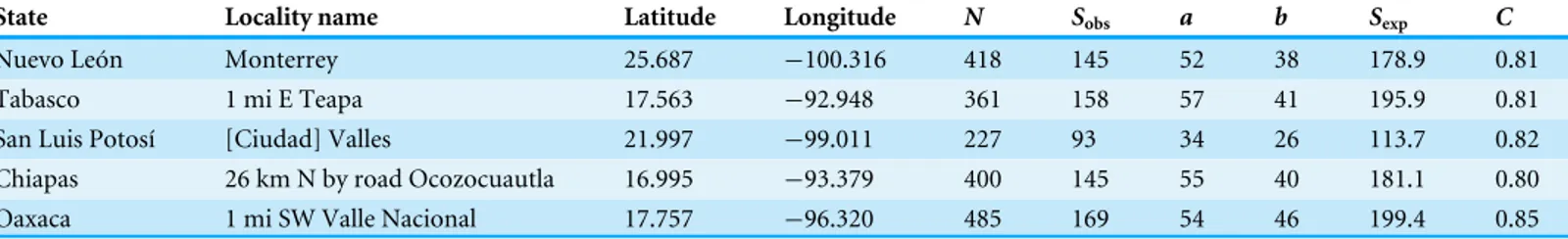
localities were rescued from among the pool of data lacking geographic coordinates, but that were inventoried completely to the level ofC≥0.8 (Table 3).
Seeking ‘hotspots’ of sampling (i.e., sets of contiguous 0.05◦pixels), we identified an
Table 3 Summary of additional sites that were ‘rescued’ from among digital data lacking geographic coordinates, but that were detected based on unique locality descriptors.
State Locality name Latitude Longitude N Sobs a b Sexp C
Nuevo León Monterrey 25.687 −100.316 418 145 52 38 178.9 0.81
Tabasco 1 mi E Teapa 17.563 −92.948 361 158 57 41 195.9 0.81
San Luis Potosí [Ciudad] Valles 21.997 −99.011 227 93 34 26 113.7 0.82
Chiapas 26 km N by road Ocozocuautla 16.995 −93.379 400 145 55 40 181.1 0.80
Oaxaca 1 mi SW Valle Nacional 17.757 −96.320 485 169 54 46 199.4 0.85
C≥0.9 completeness criterion (Xalapa, Veracruz; El Triunfo, Chiapas; Isla Cozumel,
Quintana Roo); another 17 fell at the lowerC≥0.8 criterion (Table 4). These hotspots
covered areas ranging from 60.5–4325.8 km2, considerably larger than the∼30 km2of the
0.05◦pixels. The hotspots, once again, ranged across the country, from southern Sonora
to Chiapas and Quintana Roo (Fig. 3).
DISCUSSION
This contribution is an exploration of the utility of the existing Digital Accessible Knowledge (Sousa-Baena, Garcia & Peterson, 2013) for Mexican birds in identifying well-inventoried sites across the country. We chose our 1980 cut-off to coincide roughly with the transition between initial (subtle) climate changes and the present phase of rapid, large-scale climate change worldwide (IPCC, 2013). In this way, the sites that we have identified provide baseline points of reference for species composition, for comparison with species composition later, decades into the processes of global climate change (Tingley et al., 2009).
One could map the species diversity that has been documented or that we have estimated for 0.05◦grid squares and/or hotspots across the country, to obtain a picture of species
diversity countrywide. We have avoided this temptation, however, in view of the highly non-random and scattered distribution of the well-inventoried sites across the country. The sites do not cover all regions of the country at all consistently, so any the results would be incomplete and potentially misleading. That step was, quite simply, not among the objectives of this study.
Rather, our aim was to compile a catalog of sites across Mexico that have been inventoried historically in detail, to the point that the inventory is more or less complete. This catalog, in and of itself, is not of great interest scientifically; however, to the extent that new inventories can be developed for comparison with the old ones, the interest in the comparisons grows considerably. Echoing our earlier contribution (Peterson et al., 2015), we are fascinated by the long-term processes of population biology and biogeography that are leading to turnover of species at sites.
We have improved on our earlier contribution (Peterson et al., 2015), however, which had to aggregate occurrence data to coarse resolutions (1◦, or∼110 km) until inventories
were sufficiently complete. Here, in contrast, we have sought single sites (0.05◦ grid
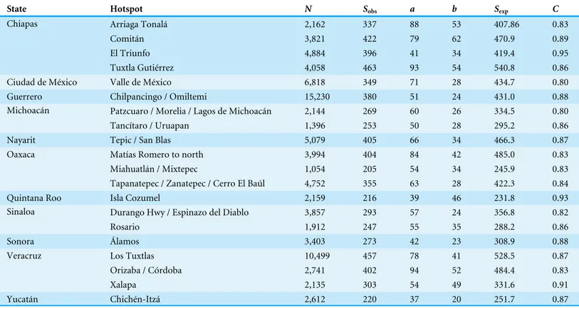
Table 4 Hotspots of sampling that are relatively completely inventoried (i.e.,C≥0.8). Hotspot names correspond to the shapefile dataset
sum-marizing the geographic distribution of these sites.
State Hotspot N Sobs a b Sexp C
Arriaga Tonalá 2,162 337 88 53 407.86 0.83
Comitán 3,821 422 79 62 470.9 0.89
El Triunfo 4,884 396 41 34 419.4 0.95
Chiapas
Tuxtla Gutiérrez 4,058 463 93 54 540.8 0.86
Ciudad de México Valle de México 6,818 349 71 28 434.7 0.80
Guerrero Chilpancingo / Omiltemi 15,230 380 51 24 431.0 0.88
Patzcuaro / Morelia / Lagos de Michoacán 2,144 269 60 26 334.5 0.80
Michoacán
Tancítaro / Uruapan 1,396 253 50 28 295.2 0.86
Nayarit Tepic / San Blas 5,079 405 66 34 466.3 0.87
Matías Romero to north 3,994 404 84 42 485.0 0.83
Miahuatlán / Mixtepec 1,054 205 54 34 245.9 0.83
Oaxaca
Tapanatepec / Zanatepec / Cerro El Baúl 4,752 355 63 28 422.3 0.84
Quintana Roo Isla Cozumel 2,159 216 39 46 231.8 0.93
Durango Hwy / Espinazo del Diablo 3,857 293 57 24 356.8 0.82
Sinaloa
Rosario 1,912 247 55 35 288.2 0.86
Sonora Álamos 3,403 273 42 23 308.9 0.88
Los Tuxtlas 10,499 457 78 41 528.5 0.87
Orizaba / Córdoba 2,741 402 94 52 484.4 0.83
Veracruz
Xalapa 2,135 303 54 49 331.6 0.91
Yucatán Chichén-Itzá 2,612 220 37 20 251.7 0.87
Alamos
Durango Hwy
Rosario
Tepic
Tancitaro Patzcuaro
Chilpancingo
Valley of Mexico
Xalapa Orizaba
Los Tuxtlas
Miahuatlan Matias Romero
Tapanatepec Arriaga
El Triunfo Tuxtla Gutierrez
Comitan Chichen-Itza
Isla Cozumel
consideration of hotspots, to some degree, began to coarsen the spatial extent of the sites once again, but offered a somewhat more extensive list of sites that have seen thorough inventories, yet still across extents much smaller than in our previous work.
One criticism that can be leveled at this work is that some important data may have been left out of the analysis. That is, the entire concept of Digital Accessible Knowledge is that the data are (1) in digital format, (2) accessible readily via the Internet, and (3) integrated with the remainder of DAK via common portals (i.e., making the transition from individual data points to integrated ‘‘knowledge’’), as was emphasized in the original publication presenting the idea of DAK (Sousa-Baena, Garcia & Peterson, 2013). (We note that a subsequent publication (Meyer et al., 2015) used ‘‘digital accessible information,’’ we believe unfortunately, as they provided no justification for or even notice of the change of terminology.) In the case of Mexican birds, for example, the Natural History Museum (UK) has very few data in digital format, and none has been made accessible, such that important collections from Mexico, like those assembled byGodman & Salvin (1879–1915), have not been analyzed in this contribution. That is the blessing and the curse of DAK: data that are digital and shared on global portals are used broadly, whereas data that do not meet the DAK criteria are frequently not used at all.
The purpose of this paper is to enable a broad suite of repeat avifaunal survey efforts across Mexico. In effect, with the maps and tables of this paper, we challenge the ornithological community interested in Mexican birds to focus attention on these sites (we provide a complete compendium of the well-inventoried sites and hotspots documented in this paper, as well as associated shapefiles, in a dataset made available permanently at http://hdl.handle.net/1808/20673). Not only does work at these sites provide information about the current community composition there, but also about the change in those communities through time.
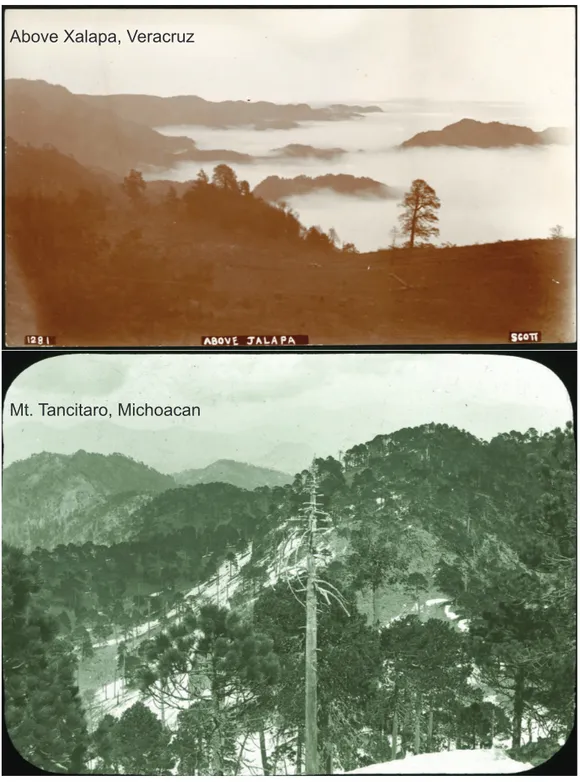
We suggest and advocate that resurvey efforts take the form of two inventories at or near the site: one in as exactly the original site as is possible to determine, and the other in the closest and most comparable site that still retains the vegetation type that was represented at the site at the time of the original inventory efforts; the former reflects effects of local-scale processes (e.g., habitat destruction, aridification), whereas the latter reflects more global processes (e.g., climate change), and comparisons of the two resurvey inventories will yield a rich understanding of the relative magnitude of effects of the local and global processes in changing avifaunas across the country. Once several such sites have been re-surveyed, a rich picture of the dynamics of Mexican bird distributions will emerge, in much greater detail than the picture presently available (Peterson et al., 2015).
Above Xalapa, Veracruz
Mt. Tancitaro, Michoacan
of landscape change have occurred at key sites (see, e.g.,Spond, Grissino-Mayer & Harley, 2014).
CONCLUSIONS
Valuable insights can be gained from longitudal comparisons to detect and characterize patterns of change in biodiversity, yet such changes have been opaque to study for lack of paired temporal samples at sites or in areas. This study explores a novel approach to enabling such studies: we mine the existing DAK for Mexican birds to detect and document well-inventoried sites, and provide a catalog of those well-known sites for others to use. Developing repeated inventories at a series of sites across Mexico would yield a detailed, controlled set of comparisons that would allow a view of avifaunal dynamics across the country. Adding the dimension of repeated landscape photography to the repeated inventories would greatly facilitate pairing of sites for future inventories at sites for which historical information exists.
ACKNOWLEDGEMENTS
We thank the Instituto de Biología and the Comisión Nacional para el Uso y Conocimiento de la Biodiversidad for generously supplying access to data.
APPENDIX
Activities, Hyogo, Japan; Museum of Southwestern Biology; Museum of Vertebrate Zoology; Museum Victoria, Australia; Natural History Museum (Bird Group, Tring); Natural History Museum of Los Angeles County; Naturalis, Amsterdam; Neotropical Ornithological Foundation; New York State Museum; North Carolina Museum of Natural Sciences; Ocean Biodiversity Information System; Ohio State University; Orcutt Trust Collection; Perot Museum of Nature and Science; Polish Academy of Sciences; Provincial Museum of Alberta; Queensland Museum; Royal Belgian Institute of Natural Sciences; Royal Ontario Museum; San Diego Natural History Museum; Santa Barbara Museum of Natural History; Senckenberg Museum; Slater Museum of Natural History; South Australian Museum; Staatliche Naturhistorische Sammlungen Dresden, Museum für Tierkunde; Staatliches Museum für Naturkunde, Stuttgart; Tall Timbers Research Station and Land Conservancy; Texas A&M University; Tulane University; U.S. National Museum of Natural History; Uberseemuseum, Bremen; Universidad Autónoma de Baja California; Universidad Autónoma de Baja California Sur; Universidad Autónoma de Campeche; Universidad Autónoma de Nuevo León; Universidad Autónoma de San Luis Potosí; Universidad Autónoma de Tamaulipas; Universidad Autónoma del Estado de Hidalgo; Universidad Autónoma del Estado de México; Universidad Autónoma del Estado de Morelos; Universidad de Ciencias y Artes de Chiapas; Universidad de Guanajuato; Universidad de Navarra; Universidad Juárez Autónoma de Tabasco; Universidad Juárez del Estado de Durango; Universidad Michoacana de San Nicolás de Hidalgo; University Museum of Zoology, Cambridge; University of AL; University of Alaska Museum; University of Alberta; University of Arizona; University of British Columbia; University of California, Davis; University of California, Los Angeles; University of Colorado; University of Iowa; University of Kansas; University of Michigan Museum of Zoology; University of Nebraska State Museum; University of Oklahoma; University of Oslo; University of Texas El Paso; University of Wyoming; Utah Museum of Natural History; Washington State University; Western Foundation of Vertebrate Zoology; Western New Mexico University; Yale Peabody Museum; Yamashina Institute of Ornithology; Zoologische Staatssammlung München; and Zoologischen Sammlung der Universitat Rostock.
ADDITIONAL INFORMATION AND DECLARATIONS
Funding
Grant Disclosures
The following grant information was disclosed by the authors: CONACyT: 152060.
Fulbright Specialists.
Competing Interests
The authors declare there are no competing interests.
Author Contributions
• A. Townsend Peterson conceived and designed the experiments, performed the
experiments, analyzed the data, wrote the paper, prepared figures and/or tables, reviewed drafts of the paper.
• Adolfo G. Navarro-Sigüenza conceived and designed the experiments, performed the
experiments, prepared figures and/or tables, reviewed drafts of the paper.
• Enrique Martínez-Meyer conceived and designed the experiments, performed the
experiments, reviewed drafts of the paper.
Data Availability
The following information was supplied regarding data availability:
KU ScholarWorks (http://hdl.handle.net/1808/20674) provides a full synonymy of locality names in relation to the hotspots identified in this paper.
GIS shapefiles showing the two sets of hotspots identified in this paper can be found at http://hdl.handle.net/1808/20673.
REFERENCES
AOU. 1998.Check-list of North American Birds. 7th edition. Washington, D.C: American Ornithologists’ Union.
Colwell RK. 1994–present.EstimateS. Storrs: University of Connecticut.
Colwell RK, Coddington JA. 1994.Estimating terrestrial biodiversity through extrapola-tion.Philosophical Transactions of the Royal Society of London B335:101–118.
Gill F, Donsker D. 2014.IOC World Bird List. Version 4.3.DOI 10.14344/IOC.ML.4.3.
Goldman EA. 1951.Biological Investigations in Mexico.Smithsonian Miscellaneous Collections115:1–476.
Godman FD, Salvin O. 1879–1915.Biologia Centrali-Americana [published in 215 parts by various authors]. London: Taylor and Francis.
Grixti JC, Packer L. 2006.Changes in the bee fauna (Hymenoptera: Apoidea) of an old field site in southern Ontario, revisited after 34 years.Canadian Entomologist
138:147–164DOI 10.4039/n05-034.
Heller EL, Kerr KC, Dahlan NF, Dove CJ, Walters EL. 2016.Overcoming challenges to morphological and molecular identification ofEmpidonax flycatchers: a case study with a Dusky Flycatcher.Journal of Field Ornithology87:96–103.
Lavergne S, Mouquet N, Thuiller W, Ronce O. 2010.Biodiversity and climate change: integrating evolutionary and ecological responses of species and com-munities.Annual Review of Ecology, Evolution, and Systematics41:321–350 DOI 10.1146/annurev-ecolsys-102209-144628.
Leache AD, Helmer D-S, Moritz C. 2010.Phenotypic evolution in high-elevation populations of western fence lizards (Sceloporus occidentalis) in the Sierra Nevada Mountains.Biological Journal of the Linnean Society 100:630–641 DOI 10.1111/j.1095-8312.2010.01462.x.
Meyer C, Kreft H, Guralnick RP, Jetz W. 2015.Global priorities for an effective informa-tion basis of biodiversity distribuinforma-tions.Nature Communications6:8221.
Monroe BLJ, Sibley CG. 1993.A world check-list of birds. New Haven: Yale University Press.
Moritz C, Patton JL, Conroy CJ, Parra JL, White GC, Beissinger SR. 2008.Impact of a century of climate change on small-mammal communities in Yosemite National Park, USA.Science322:261–264DOI 10.1126/science.1163428.
Navarro-Sigüenza AG, Peterson AT. 2004.An alternative species taxonomy of Mexican birds.Biota Neotropica4:1–32.
Nelson EW. 1921.Lower California and its natural resources.Memorias of the National Academy of Sciences16:1–194.
Nilsson SG, Franzén M, Jönsson E. 2008.Long-term land-use changes and extinction of specialised butterflies.Insect Conservation and Diversity1:197–207.
Nunes MFC, Galetti M, Marsden S, Pereira RS, Peterson AT. 2007.Are large-scale dis-tributional shifts of the Blue-winged Macaw (Primolius maracana) related to climate change? Journal of Biogeography34:816–827 DOI 10.1111/j.1365-2699.2006.01663.x.
Olvera-Vital A. 2012.Avifauna del Municipio de Misantla, Veracruz. Tesis de Licenciatura. Mexico: Facultad de Ciencias, Universidad Nacional Autónoma de México.
Peters JL. 1931–1987.Check-list of birds of the world, vols. 1–16. Cambridge: Harvard University Press.
Peterson AT, Navarro-Sigüenza AG. 2005.Hundred-year changes in the avifauna of the Valley of Mexico, Distrito Federal, Mexico.Huitzil7:4–14.
Peterson AT, Navarro-Sigüenza AG. 2006.Consistency of taxonomic treatments: a re-sponse to Remsen (2005).Auk123:885–887
DOI 10.1642/0004-8038(2006)123[885:COTTAR]2.0.CO;2.
Peterson AT, Navarro-Siguüenza AG, Martínez-Meyer E, Cuervo-Robayo AP, Berlanga H, Soberón J. 2015.Twentieth century turnover of Mexican endemic avifaunas: landscape change versus climate drivers.Science Advances1:e1400071 DOI 10.1126/sciadv.1400071.
Peterson AT, Slade NA. 1998.Extrapolating inventory results into biodiversity esti-mates and the importance of stopping rules.Diversity and Distributions4:95–105 DOI 10.1046/j.1365-2699.1998.00021.x.
mammal distributions over the past century.Global Change Biology17:696–708 DOI 10.1111/j.1365-2486.2010.02297.x.
Sánchez GA. 1998.Misantla: Cultura, Tradición y Leyenda. Veracruz: Asociación para el Desarrollo Integral de la Región de Misantla, A.C.
Scholes RJ, Biggs R. 2005.A biodiversity intactness index.Nature434:45–49 DOI 10.1038/nature03289.
Soberón J, Llorente JE. 1993.The use of species accumulation functions for the predic-tion of species richness.Conservation Biology7:480–488
DOI 10.1046/j.1523-1739.1993.07030480.x.
Sousa-Baena MS, Garcia LC, Peterson AT. 2013.Completeness of Digital Accessible Knowledge of the plants of Brazil and priorities for survey and inventory.Diversity and Distributions20:369–381.
Spond MD, Grissino-Mayer HD, Harley GL. 2014.Comparing dynamics of mixed-conifer woodlands on the Bandera Lava Flow, New Mexico.Southwestern Naturalist
59:235–243DOI 10.1894/F11-JEM-01.1.
Tingley MW, Beissinger SR. 2009.Detecting range shifts from historical species occur-rences: new perspectives on old data.Trends in Ecology and Evolution24:625–633 DOI 10.1016/j.tree.2009.05.009.