www.ocean-sci.net/12/1205/2016/ doi:10.5194/os-12-1205-2016
© Author(s) 2016. CC Attribution 3.0 License.
A stable Faroe Bank Channel overflow 1995–2015
Bogi Hansen1, Karin Margretha Húsgarð Larsen1, Hjálmar Hátún1, and Svein Østerhus2 1Faroe Marine Research Institute, P.O. Box 3051, 110 Tórshavn, Faroe Islands
2Uni Research Climate, Nygårdsgata 112, 5008 Bergen, Norway
Correspondence to:Bogi Hansen ([email protected])
Received: 15 July 2016 – Published in Ocean Sci. Discuss.: 4 August 2016
Revised: 11 October 2016 – Accepted: 27 October 2016 – Published: 17 November 2016
Abstract.The Faroe Bank Channel (FBC) is the deepest pas-sage across the Greenland–Scotland Ridge (GSR) and there is a continuous deep flow of cold and dense water passing through it from the Arctic Mediterranean into the North At-lantic and further to the rest of the world ocean. This FBC overflow is part of the Atlantic Meridional Overturning Cir-culation (AMOC), which has recently been suggested to have weakened. From November 1995 to May 2015, the FBC overflow has been monitored by a continuous ADCP (acous-tic Doppler current profiler) mooring, which has been de-ployed in the middle of this narrow channel. Combined with regular hydrography cruises and several short-term moor-ing experiments, this allowed us to construct time series of volume transport and to follow changes in the hydrographic properties and density of the FBC overflow. The mean kine-matic overflow, derived solely from the velocity field, was found to be (2.2±0.2) Sv (1 Sv=106m3s−1)with a slight, but not statistically significant, positive trend. The coldest part, and probably the bulk, of the FBC overflow warmed by a bit more than 0.1◦C, especially after 2002, increasing the transport of heat into the deep ocean. This warming was, however, accompanied by increasing salinities, which seem to have compensated for the temperature-induced density de-crease. Thus, the FBC overflow has remained stable in vol-ume transport as well as density during the 2 decades from 1995 to 2015. After crossing the GSR, the overflow is modi-fied by mixing and entrainment, but the associated change in volume (and heat) transport is still not well known. Whatever effect this has on the AMOC and the global energy balance, our observed stability of the FBC overflow is consistent with reported observations from the other main overflow branch, the Denmark Strait overflow, and the three Atlantic inflow branches to the Arctic Mediterranean that feed the overflows. If the AMOC has weakened during the last 2 decades, it is
not likely to have been due to its northernmost extension – the exchanges across the Greenland–Scotland Ridge.
1 Introduction
Overflow is the term generally used to describe the bottom-intensified flow of cold and dense water from the Nordic seas through the deep passages across the Greenland–Scotland Ridge (GSR) to the North Atlantic (Saunders, 2001). The strongest overflow branch in terms of volume transport passes through the Denmark Strait. The Denmark Strait overflow (DS overflow) is estimated to transport around 3.5 Sv (1 Sv=106m3s−1)of dense (σ
θ> 27.8 kg m−3) wa-ter (Jochumsen et al., 2012; Harden et al., 2016). A simi-lar amount of overflow is generally considered to pass east of Iceland in three branches where the overflow across the Wyville Thomson Ridge is weak (< 0.3 Sv; Østerhus et al., 2008). The overflow across the Iceland–Faroe Ridge (IFR overflow) is not well constrained by observations despite considerable effort (Beaird et al., 2013; Olsen et al., 2016).
The third overflow branch east of Iceland is the deep flow through the Faroe Bank Channel (FBC), FBC overflow, which is the main focus of this study. With a sill depth of 840 m, the FBC is by far the deepest passage across the GSR and one of the main pathways for the cold and dense overflow waters generated in the Arctic Mediterranean (Fig. 1). With an average volume transport close to 2 Sv, the FBC overflow is generally estimated to contribute ca. one-third of the total overflow, and is second only to the DS overflow (Østerhus et al., 2008).
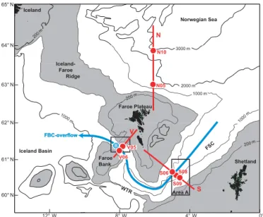
Figure 1.Map of the region with gray areas shallower than 500 m. Blue arrow indicates the path of the FBC overflow through the Faroe–Shetland Channel (FSC), after which it is turned northwest-wards by the Wyville Thomson Ridge (WTR) to flow through the FBC between the Faroe Plateau and Faroe Bank. Red lines indicate three standard sections (V, S, and N) with selected standard CTD stations indicated by red circles. Blue circle labeled “B” indicates the long-term mooring site FB over the sill of the FBC. Black rect-angle over the sill and section V show area that is illustrated in more detail in Fig. 2. Black rectangle over section S shows area A, from which CTD stations deeper than 600 m have been analyzed.
product less dense than the DS overflow. If there is no signifi-cant detrainment (Mauritzen et al., 2005), the entrainment of ambient waters should increase the volume transport of the FBC overflow on its passage from the FBC to the deep west-ern boundary current in the Labrador Sea. This would make it one of the main contributors to the formation of North Atlantic Deep Water (NADW) and the lower limb of the Atlantic Meridional Overturning Circulation (AMOC). The FBC overflow transports oxygen, heat, and anthropogenic carbon dioxide absorbed from the atmosphere into deeper parts of the world oceans (Sabine et al., 2004) and it is one of the processes that generates the driving force for the warm Atlantic inflow to the Arctic Mediterranean (Hansen et al., 2010).
The FBC overflow is therefore an important component of the ocean circulation and climate system and it has been the focus of many different studies through the years (e.g., Her-mann, 1967; Borenäs and Lundberg, 1988; Saunders, 1990; Hansen and Østerhus, 2007; Olsen et al., 2008). Many at-tempts have also been made to determine its volume trans-port as reviewed by Saunders (2001), Hansen and Øster-hus (2000), and Hansen and ØsterØster-hus (2007). Most of them are consistent with the values presented by Hansen and Østerhus (2007). For the 1995 to 2005 period, they estimated the average volume transport of kinematic overflow, derived
solely from the velocity field, to be (2.1±0.2) Sv, whereas the volume transport of dense (σθ> 27.8 kg m−3)FBC over-flow was (1.9±0.3) Sv. We will frequently cite results from this study and will hereafter refer to it as “HØ2007”.
In the present study, we do not aim towards refining this es-timate. Rather, we will study the long-term variations, mainly to see whether there are any systematic changes. The main motivation for this is the link between the FBC overflow and the AMOC. Climate models have long projected AMOC weakening (Collins et al., 2013) and recently there have been reports that this weakening has already started (Smeed et al., 2014; Robson et al., 2014; Rahmstorf et al., 2015).
A weakened AMOC could be due to weaker deepwa-ter formation in the wesdeepwa-tern North Atlantic, especially the Labrador Sea (Robson et al., 2014), but Smeed et al. (2014) found that their observed 2004–2012 decrease was due to “a decrease in the southward flow of lower NADW below 3000 m”, which they consider to be fed from the overflows.
Motivated by this, the main aim of this study is to analyze our observational data set from the FBC, initiated in Novem-ber 1995, to see whether there are any indications of a weak-ening or other systematic changes. The observations include continuous monitoring of the velocity field with moored AD-CPs (acoustic Doppler current profilers), regular hydrogra-phy cruises, and short-term dedicated mooring experiments.
During the first years of observation, there were indica-tions of a weakened FBC overflow, consistent with long-term hydrographic changes observed at Ocean Weather Station M in the Norwegian Sea. This led to the suggestion of a long-term weakening of the FBC overflow (Hansen et al., 2001), which was refuted by HØ2007 and by Olsen et al. (2008). In-stead, the first 10 years of observation showed a remarkable stability in overflow transport. Since then, the observational period has been doubled and we present for the first time an analysis of the changes in FBC overflow for the full observa-tional period up to May 2015.
Following HØ2007, our main time series for overflow transport is the kinematic overflow. This parameter is based on the velocity field, solely, and can be derived from the ADCP measurements. This parameter does not, however, provide a complete picture of the overflow since its temper-ature and salinity characteristics could vary even if the kine-matic overflow does not, and, in particular, the density of the overflow may affect the AMOC.
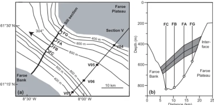
Figure 2. (a)Map showing the sill section with ADCP sites indi-cated by circles and the standard hydrographic section (section V) with standard stations indicated by black squares. The shaded area is shallower than 300 m.(b) The sill section with ADCP sites is indicated. The shaded area indicates a typical variation of the inter-face.
On its way from the FBC to the deep western boundary current, the FBC overflow mixes with and entrains water from the Atlantic side of the GSR. The associated change in hydrographic properties has been well documented (e.g., Fogelqvist et al., 2003), but the change in volume transport is more difficult to estimate, which means that the contribution of modified FBC overflow to NADW and to the AMOC is less well known. Here, we do not aim to solve that question, but we discuss the state of our understanding of this topic.
2 Material and methods
We use observations from moored instrumentation and from ship-borne CTD (conductivity, temperature, depth) observa-tions. The moorings have all been deployed over the sill (Fig. 2a). The CTD data are mainly from selected stations on three regularly occupied standard sections as well as an area in the Faroe–Shetland Channel (FSC), all of them shown in Fig. 1. In this section, we also describe the method used for estimating kinematic overflow and some statistical methods.
2.1 Data from moored instrumentation
ADCP moorings have been deployed at four different sites along a section over the sill of the channel (Fig. 2). The dominant location is site FB, which has been occupied since November 1995 except for annual (2–3 weeks) servicing in-tervals and gaps due to mooring or instrument failure. The ADCP data at this site comprise 6750 days of velocity pro-files (with 72 propro-files, “pings”, per day), all of them having at least 16 “bins” of 25 m height, i.e., reaching at least 400 m above the bottom and thus well above the overflow layer ex-cept for a few days (≈0.2 %).
At site FC, regular deployments were initiated in summer 2002 and have continued in most years since then although with gaps. The other two sites have only had one
deploy-ment each, lasting 70 days at FA, and 364 days at FG. At most sites, the ADCP was located in the top of a traditional (very short) mooring, but the ADCP at site FG was located in a bottom mounted frame to protect it from fishing gear. A complete list of ADCP deployments is in a technical re-port (Hansen et al., 2015a), available online, which also lists details and discusses the quality of these measurements.
In addition to velocity profile the ADCP measures temper-ature at the instrument. This sensor may have an offset of several tenths of a degree, but comparison to simultaneous CTD profiles allows for a calibrated temperature series to be generated with an accuracy of ca. 0.05◦C (HØ2007). After the summer of 2001, a SeaBird MicroCat (SBE37) instru-ment, which measures temperature more accurately, was at-tached to the ADCP. The MicroCats have been regularly cal-ibrated either at the factory or by being attached to a SeaBird 911plus CTD that is lowered and kept for some time at a depth with stable temperature. None of the calibrations have shown a larger drift than a few millidegrees. Since July 2001, the bottom temperature series at FB therefore has been accu-rate within 0.01◦C, at least.
The MicroCat also measures conductivity, from which salinity may be derived, but evaluation of the data has gener-ally led to the conclusion that the uncertainty of these mea-surements is too high to yield useful results, perhaps due to contamination in this bottom-near high-turbulence regime. Thus, we do not use these data here.
2.2 Data from CTD profiles
We mainly use CTD data from the period 1996 to 2015. These have been acquired with a SeaBird SBE911plus sys-tem with double sys-temperature and conductivity sensors. Tem-perature has been calibrated at the factory annually and salin-ity has been calibrated ashore by salinometer (Autosal) anal-ysis of water samples acquired in triples, generally at every profile. For the deep, weakly stratified, waters mainly con-sidered here, the typical accuracy is estimated at 0.001◦C for temperature and 0.002 for salinity. These values may not hold for individual profiles, but for the averages, considered in this study, they should be representative. All salinity val-ues are presented as practical salinities.
In order to relate the deepwater changes to changes in the upper layers, we also use time series of temperature and salinity in the cores of Atlantic water (defined by maximum salinity) on sections V and N, derived from de-seasoned CTD observations. These series are updated from Larsen et al. (2012).
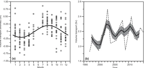
Figure 3.Seasonal(a)and long-term(b)variations of kinematic overflow 1995–2015.(a)Each square represents transport deviation for 1 month from the 3-year-running mean. The curve represents the iteratively determined sinusoidal seasonal fit.(b)Annually averaged transport excluding days 136–195 (dashed curve) and 3-year-running mean transport (continuous curve) with the shaded area representing±1 standard error over each 3-year period.
ADCP was sufficient to generate a time series of kinematic overflow, especially on timescales of a month or longer. This was to be expected since the deep parts of the FBC are nar-row over the sill, with a width on the order of the baro-clinic Rossby radius. The cross-channel variations of the along-channel velocity are highly correlated on timescales of months or longer (HØ2007).
By definition, kinematic overflow is the volume trans-port below the interface, which is defined from the veloc-ity field (Supplement Fig. S1), integrated across the channel. Based on the horizontal co-variation, HØ2007 developed al-gorithms to calculate kinematic overflow from the daily aver-aged velocity profile at site FB. This involved both inter- and extrapolation and, especially, the horizontal extrapolation to-wards the Faroe Plateau introduced some uncertainty.
With the new ADCP measurements at site FG (Fig. 2), this uncertainty can be reduced and the algorithms adapted. This has been done in the previously cited technical re-port (Hansen et al., 2015a) and a new time series of kine-matic overflow has been generated for the whole period. For monthly averages, the correlation coefficient between the new and the old series is 0.92 and the overall averages only differed by 1 %. HØ2007 estimated the uncertainty of the kinematic overflow to be 0.2 Sv. With the adapted algo-rithm, this uncertainty has not increased and we will retain this value.
There are other ways to define and calculate a kinematic overflow. The standard interface is at the depth where the along-channel velocity has been reduced to 50 % of the core velocity (Fig. S1). Instead, we could define a baroclinic in-terface to be at the depth where the along-channel velocity has been reduced to 50 % of the velocity difference between
the core and the upper layer, which we represent with bin 16. The effect of this modification may be estimated by calcu-lating the transport density; i.e., the velocity integrated up to the interface for these two definitions. For annual averages the baroclinic interface would give transport densities highly correlated with those for the standard interface (R=0.998) and only 0.5 % higher in overall average (Fig. S2).
A third alternative would be to keep a fixed interface at the top of bin 16. This alternative would give an overall av-erage 5 % higher than the standard, but annual transport den-sities (Fig. S2) would still be highly correlated with the stan-dard definition (R=0.984). Although different definitions of kinematic overflow may give different average transports, this indicates that long-term variations and hence trends will be very similar.
2.4 Statistical methods
de-seasoned values within each 3-year period. This also allows us to calculate the standard error of each 3-year mean value. We will investigate temporal trends for several different parameters by linear trend analysis, which is done by stan-dard linear regression analysis of the parameter on time. In general, we will report the trend as the regression slope±its 95 % confidence interval as determined by a standardttest.
The statistical significance of standard errors in the itera-tive decomposition method and confidence limits in the trend analysis depends on assumptions of serial correlation and normal distributions, which may not always be valid. There-fore, we do not claim specific statistical confidence levels for the reported values, although in some cases we use them to claim lack of significance.
3 Results
3.1 Overflow volume transport
Monthly averaged kinematic overflow values (Fig. S3) ranged from 1.2 to 3.2 Sv. In Fig. 3, the variations are split into 3-year-running mean values (Fig. 3b) and deviations (anomalies) from these (Fig. 3a), as described in Sect. 2.4. As noted by HØ2007, the transport anomalies have a sea-sonal variation with maximum in August. Also shown is the annually averaged transport excluding days 136–195, during which period the servicing gap in different years occurred. The overall average transport was 2.2 Sv and the linear trend was (0.010±0.013) Sv yr−1. The annual averages (dashed curve in Fig. 3b) do not indicate strong serial correlation, but taking that into account can only increase the uncertainty. Thus, we see no statistically significant trend in the kinematic overflow and the indication is of a strengthening rather than a weakening.
3.2 Bottom temperature
The main data set for overflow temperature is the time series of temperature measured by the ADCP until summer 2001 and by the attached MicroCat after that. The instrument depth has varied slightly from one deployment to another, but has been close to a typical depth of 810 m. This depth is around 30 m shallower than the sill depth and site FB is also dis-placed some 3 km northeast of the deepest part of the sill (Fig. 2). The question therefore arises, how well does this time series represent the bottom water over the sill.
The effect of vertical displacement may be estimated by considering how the temperature varies with depth from 840 m upwards at standard station V06 (Fig. S4a). Station V06 is around 25 km upstream of the sill (Fig. 2a) and we may expect some change to the vertical structure as the over-flow water accelerates towards the sill. Nevertheless, the bias introduced by the vertical displacement is not likely to ex-ceed a few hundredths of a degree. Also, the relatively small standard error (Fig. S4a) indicates that the bias should be
constant within±0.01◦C as long as we are considering tem-porally averaged values.
Similarly, the effect of the horizontal displacement may be estimated by comparing the bottom temperature at FB with simultaneously (same-day) measured temperature at 810 m depth at station V06 (Fig. S4b). The correlation coefficient was 0.69 with a regression coefficient of 0.69±0.19. This indicates that the bottom temperature at FB varies a bit less than temperature at the same depth at V06. On average, the water at 810 m depth at V06 was (0.045±0.011)◦C colder than the bottom water at FB.
Altogether, we may conclude that the coldest water flow-ing over the sill is probably somewhat colder than the bot-tom temperature measured at FB and this bias may well be on the order of 0.05◦C. When averaged over long periods, especially over a year, this bias seems, however, to be fairly constant with an uncertainty on the order of 0.01◦C. Thus, variations observed at FB ought to represent the bottom wa-ter within this uncertainty. In the following, we will use the measurements at FB as representing the bottom temperature at the FBC sill with this caveat.
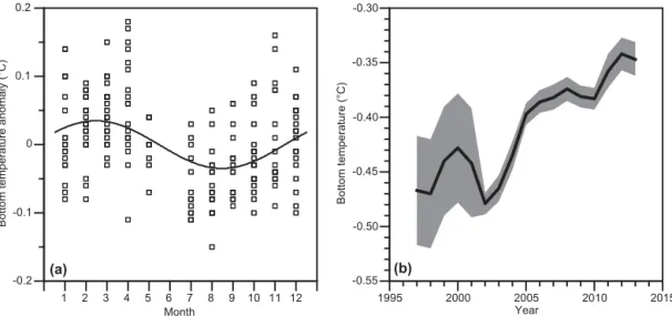
The bottom temperature measurements at site FB were av-eraged to monthly values, excluding months with less than 28 days. With the method in Sect. 2.4, they were split into a 3-year-running mean bottom temperature (Fig. 4b) and the monthly deviations (anomalies) from these (Fig. 4a). The monthly anomalies indicate a seasonal variation with mini-mum temperature in August as previously noted (HØ2007). The 3-year-running mean (Fig. 4b) has a clear positive trend, especially after 2002. The shaded area on Fig. 4b indicates the uncertainty of the 3-year-running mean, estimated as±1 standard error over each 3-year period, but not smaller than the instrumental uncertainty, which is±0.05◦C prior to sum-mer 2001 and±0.01◦C after that.
An objective estimate of the bottom temperature change at FB can be obtained by a linear trend analysis (regress-ing annually averaged bottom temperature on time). For the whole period 1996 to 2014, this gives a warming of (0.10±0.06)◦C. Using only the measurements after Micro-Cats were introduced in 2001 gives almost identical results. The high uncertainty before 2001 makes it difficult to ascer-tain the temperature variation in the early years, but Fig. 4b does not indicate that it was appreciably colder in this period than in 2002. Thus, the bottom temperature at FB most likely increased by a bit more than 0.1◦C during our observational period.
Figure 4.Seasonal(a)and long-term(b)variations of bottom temperature at FB 1995–2015.(a)Each square represents the deviation for 1 month from the 3-year-running mean. The curve represents the iteratively determined sinusoidal seasonal fit;(b)3-year-averaged transport (black curve) with the shaded area representing the uncertainty interval.
3.3 Salinity and density changes
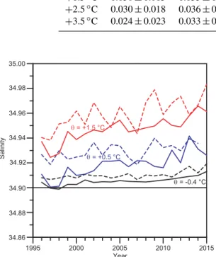
By itself, a warming of the bottom water would imply re-duced density, but density also depends on the salinity. Thus, we need to consider possible salinity changes of the FBC overflow. Unfortunately, our salinity measurements over the sill of the FBC are not adequate to clarify this, but we have regular CTD measurements from regions close to and far-ther upstream of the sill. The FBC overflow is fed from the deep layers of the FSC, but it experiences intensive mixing on its way towards and over the FBC sill (Saunders, 1990; Mauritzen et al., 2005). Standard section V (Fig. 1) has only two stations that reach sufficient depths to cover the overflow (Fig. 2a) and theirθ–Srelationships are illustrated in Fig. 5 together withθ–Straces from two stations in the FSC.
The two stations from the FSC in Fig. 5 are on oppo-site sides of the channel (Fig. 1), but the data are only from cruises with occupations of both stations. Therefore, the fact that their θ–S traces are almost indistinguishable (Fig. 5b) shows that they represent the average conditions of the FSC waters feeding the FBC overflow through this period (sta-tion S09 has not been regularly occupied since 2010). The twoθ–Straces from section V are averages for the same pe-riod, although more frequently occupied. Therefore, their dif-ferences from the FSCθ–Straces indicate substantial water mass changes occurring during the flow between the two sec-tions.
Figure 5 also shows that the twoθ–Straces from section V are different. Here, again, we have only used data where both stations were occupied during the same cruise (i.e., within a few hours) and so the lack of overlap between the shaded areas surrounding the traces in Fig. 5b implies that the differ-ence is real. This differdiffer-ence has been ascribed to the different occurrences of a “third water mass” (Borenäs et al., 2001;
Borenäs and Lundberg, 2004). However, both V05 and V06 show differentθ–S relationships from the source waters in the FSC and HØ2007 argued that this was more likely due to more intensive mixing of the water arriving at V06.
The changes in θ–S relationship from the FSC to the FBC may involve both internal mixing within the overflow layer and admixing of upper layer waters. Temporal salinity changes in the FBC could therefore derive from changes in the upstream overflow waters or from local mixing of chang-ing upper layer waters. In the followchang-ing, we first consider the conditions on section V, slightly upstream of the sill, and then in the FSC and farther upstream. After that, we consider the effects of local mixing.
3.3.1 Salinity and density changes on section V
For the period 1996 to 2015, there are almost a hundred oc-cupations of V05 and V06, and Table 1 lists overall changes of temperature, salinity, and potential density in different depth layers at these two stations during this period. The ta-ble shows increased temperatures and salinities at almost all depths, although some of the changes are not significantly different from zero.
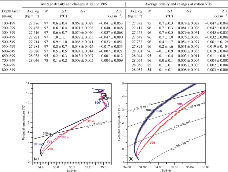
Table 1.Overall change from 1996 to 2015 according to linear trend analyses for various depth layers at stations V05 and V06. For each layer, the table shows average potential density (avg.σθ), number of CTD occupations (N), and changes in temperature (1T), salinity (1S), and potential density (1σθ).
Average density and changes at station V05 Average density and changes at station V06
Depth layer Avg.σθ N 1T 1S 1σθ Avg.σθ N 1T 1S 1σθ
(m–m) (kg m−3) (◦C) (kg m−3) (kg m−3) (◦C) (kg m−3)
100–199 27.386 97 0.6±0.4 0.067±0.029 −0.041±0.053 27.372 95 0.7±0.3 0.079±0.027 −0.047±0.048 200–299 27.438 97 0.6±0.4 0.071±0.028 −0.040±0.048 27.417 96 0.7±0.3 0.081±0.026 −0.042±0.038 300–399 27.516 97 0.6±0.7 0.070±0.040 −0.037±0.068 27.455 96 0.7±0.5 0.079±0.031 −0.045±0.053 400–499 27.721 97 1.0±1.1 0.089±0.055 −0.047±0.080 27.548 96 0.7±1.0 0.076±0.050 −0.032±0.089 500–549 27.914 97 0.9±1.0 0.068±0.041 −0.023±0.051 27.732 96 0.4±1.7 0.054±0.077 0.001±0.126 550–599 27.981 97 0.8±0.7 0.048±0.025 −0.017±0.033 27.891 96 0.2±1.6 0.031±0.069 0.019±0.104 600–649 28.020 97 0.5±0.5 0.024±0.014 −0.007±0.021 28.001 96 −0.1±0.9 0.008±0.035 0.019±0.048 650–699 28.038 95 0.2±0.3 0.013±0.007 −0.001±0.012 28.044 95 −0.1±0.4 0.003±0.011 0.011±0.015 700–749 28.046 78 0.1±0.2 0.009±0.005 0.004±0.009 28.054 96 0.0±0.1 0.005±0.004 0.004±0.005 750–799 28.056 85 0.1±0.1 0.006±0.003 0.002±0.004 800–849 28.057 54 0.1±0.1 0.008±0.004 0.003±0.006
Figure 5.θ–Sdiagrams for four standard stations based on 73 occupations at stations V05 (magenta) and V06 (red) simultaneously and on 54 occupations at stations S06 (blue) and S09 (black) simultaneously in the period 1996–2010.(a)Averageθ–Straces for the whole water column with conditions at 500 m depth indicated by circles.(b)Expanded view of waters colder than 5◦C with the average for each station shown as a colored line surrounded by a shaded area in the same color representing the average±1 standard error. Station locations are shown on Figs. 1 and 2a.
To circumvent this, we may use the fact that salinity and potential density change much more regularly at fixed po-tential temperature (θ )than at fixed depth. This allows us to determine salinity changes for various values ofθ. Com-bined with time series of θ at fixed depth, this gives time series of salinity and potential density at fixed depth. In par-ticular, combination with the continuous measurements ofθ
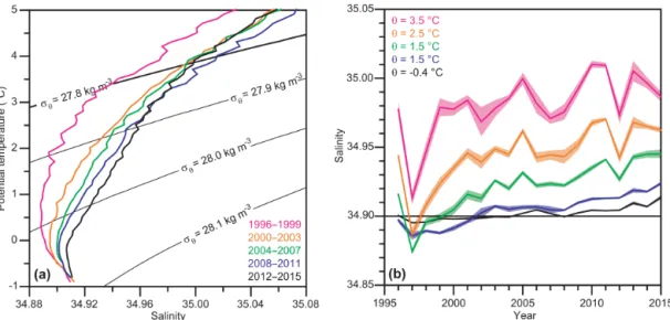
at FB allows for more accurate determination of the density change at the bottom. In Fig. 6, salinity variations are shown for three different values of θ within the overflow layer of section V. The time series are fairly noisy, but all of them indicate increasing salinity trends, which are confirmed by linear trend analysis (Table 2). The last three columns in
Ta-ble 2 also show that to compensate for the salinity increases in the table, substantial increases in potential temperature are required.
disap-Table 2.Salinity increase at five fixed potential temperatures (θ )from 1996 to 2015 based on linear trend analyses for two stations on section V and stations in area A in the FSC (Fig. 1). The last three columns show the change in potential temperature that would be required to compensate for the salinity change with respect to potential density.
Salinity change 1996–2015 Compensatingθchange
θ V05 V06 FSC V05 V06 FSC
−0.4◦C 0.011±0.006 0.005±0.003 0.013±0.004 0.18◦C 0.08◦C 0.21◦C
+0.5◦C 0.021±0.007 0.021±0.015 0.032±0.006 0.27◦C 0.27◦C 0.41◦C
+1.5◦C 0.030±0.013 0.033±0.018 0.050±0.014 0.32◦C 0.35◦C 0.52◦C
+2.5◦C 0.030±0.018 0.036±0.022 0.049±0.022 0.27◦C 0.33◦C 0.44◦C
+3.5◦C 0.024±0.023 0.033±0.018 0.044±0.027 0.19◦C 0.26◦C 0.35◦C
1995 2000 2005 2010 2015
34.88 34.90 34.92 34.94 34.96 34.98 35.00
34.86
Salinity
Year = +0.5 °C
= -0.4 °C = +1.5 °C
Figure 6.Temporal change of salinity at three fixed potential tem-peratures (θ ):−0.4◦C (black),+0.5◦C (blue),+1.5◦C (red) for station V05 (continuous) and V06 (dashed).
peared (Fig. 7a). For the period considered, the lowest salini-ties for fixed potential temperature were observed in 1997. After that, the salinity at all the potential temperatures in Fig. 7b started to rise. For high values ofθ, the initial salin-ity increase was rapid, followed by almost stable conditions, whereas the colder waters exhibited a more gradual salinity increase, continuing throughout the period.
In the southern region of the Norwegian Sea, observa-tions at 800 m depth on section N (Fig. 1) show water with a similar potential temperature as the bottom water at FB and the two curves show a remarkable similarity in warm-ing (Fig. 8a).
3.3.3 The effects of local mixing
In addition to warming and salinification of the source water in the Norwegian Sea, the FBC overflow water will receive heat and salt from the Atlantic layer on top by entrainment and mixing. Variations in the properties of the Atlantic water
core in the FBC (Fig. S7) will then also induce variations in the overflow water.
An estimate of this contribution may be achieved by con-sidering the changes in salinity from section S to section V (Fig. 5). According to HØ2007, the water with potential density exceeding 27.8 kg m−3on section V had a transport-averaged potential temperatureθ=0.25◦C and a salinity of 34.93 for the 1996 to 2005 period. For the FSC, the avail-able velocity measurements in the deep water do not allow us to derive transport-averaged properties for the water flow-ing from the FSC into the FBC, but we can make a rough estimate by comparing average salinities atθ=0.25◦C for this period. At S08, this value was 34.893, i.e., 0.037 less saline than over the FBC sill. If this salinity increase along the flow is obtained by admixing upper layer Atlantic wa-ter with θ=8.84◦C and S=35.31 (average properties of Atlantic core 1996–2005), then 9 % of Atlantic water is re-quired. This would also require that the overflow water in the FSC had an average potential temperature of−0.59◦C, which seems rather cold, but the bottom-near water at S08 was on average −0.78◦C and, according to Mauritzen et al. (2005), this water also feeds the FBC overflow.
Thus, an admixture of somewhere between 5 and 10 % At-lantic water seems realistic. This implies that any change in temperature or salinity of the Atlantic water should be rapidly transferred to the overflow, although reduced by a factor of 10 to 20. From 1995 to 2003, the Atlantic water core in the upper parts of the FBC warmed by ca. 0.8◦C (Fig. 8a) and increased in salinity by ca. 0.1 (Fig. S7). This may be ex-pected to have warmed the FBC overflow by 0.04 to 0.08◦C and increased its salinity by 0.005 to 0.01. After 2010, both temperature and salinity of the Atlantic water core on section V have decreased (Fig. S7).
Figure 7.Temporal variations of the water mass characteristics in the deep parts of the FSC.(a)θ–Straces averaged over consecutive 4-year periods.(b)Salinity trends for five different potential temperatures where the annual averages are shown by the colored lines surrounded by shaded areas representing average±1 standard error for each year. The figure is based on 505 CTD profiles from area A in the FSC (Fig. 1).
Figure 8. (a)Potential temperature of the Atlantic water core on section V (red, right axis), of the bottom water at FB (black, left axis), and at 800 m depth on section N (average of stations N05 to N10, blue, left axis).(b)Potential density at two fixed depths (black: 700 m and blue: 800 m) on section N (average of the six stations N05 to N10) and for the overflow layer assuming two different fractions of locally admixed Atlantic core water (green: 5 % and red: 10 %); see text. All curves are 3-year-running means with shaded areas representing average±1 standard error over each 3-year period.
More important is the question of how the local mixing may have changed the density during our observational pe-riod. This is exemplified by the red and the green curves in Fig. 8b. There, we have assumed that the average properties during the 1996 to 2005 period, as cited above, came about as a mixture of cold water from the FSC and Atlantic wa-ter in fraction 5 (green) or 10 % (red), respectively. Assum-ing further that the mixAssum-ing fractions as well as the cold water properties in the FSC remained unchanged, the red and green curves in Fig. 8b show how the density of this mixture would vary in time.
4 Discussion
The main aim of this study has been to determine whether the FBC overflow has experienced any systematic changes dur-ing the observational period from November 1995 to May 2015, and especially to ask whether there has been any change that could help explain reports of a weakened AMOC (e.g., Smeed et al., 2014). We have split this question into two parts: (1) has the volume transport of the overflow changed and (2) have the properties (temperature or salinity and espe-cially the density) of the overflow changed. In the next two sections, we summarize our results in an attempt to answer those two questions. We then briefly try to summarize our present understanding of the modifications that the overflow experiences from the FBC sill on its way towards the AMOC, followed by a discussion of the wider implications of our re-sults.
4.1 Observed changes of overflow volume transport
Monthly averaged kinematic overflow was calculated for all months with observational coverage (200 out of a total of 233 months) between December 1995 and April 2015. The calculations used the method described in HØ2007, slightly adapted based on new observations as detailed in Hansen et al. (2015a). The resulting time series (Figs. S3 and 3) did not exhibit any obvious systematic changes ex-cept perhaps a weak increase, and a linear trend analysis gave (0.010±0.013) Sv yr−1. As shown in Sect 2.3 and Fig. S2, different definitions of kinematic overflow might give differ-ent average transports, but are not likely to affect the long-term variation and hence trend appreciably.
Although defined purely from the velocity field, the mo-tivation for considering the kinematic overflow is based on the assumption that its variations also reflect variations in the transport of overflow water as defined in terms of tempera-ture or density. This is not easy to prove conclusively since it requires simultaneous velocity and hydrography observa-tions covering the same section adequately over a prolonged period. Based on the observations up to 2005, HØ2007 con-cluded that there is such a relationship.
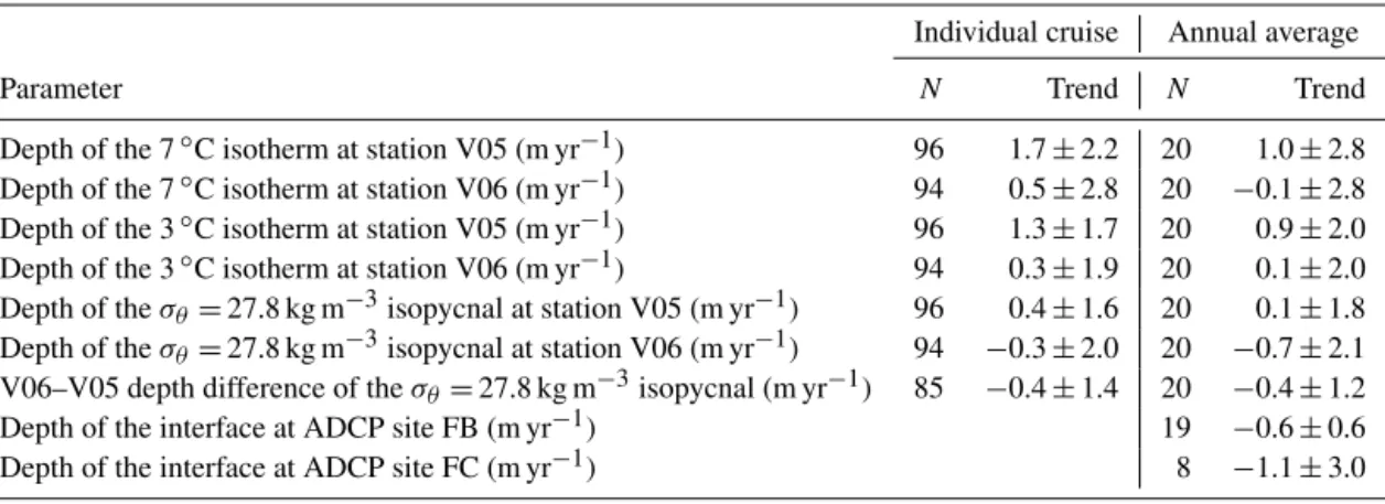
Since then, the mooring at ADCP site FG has provided a time series of bottom temperature over the slope on the Faroe side of the channel. This series is positively correlated with an interface depth at FB (Table S1), especially on long timescales, which supports the relationship. Additional hy-drographic observations are mainly from section V, which is more than 20 km upstream of the sill section, where velocity has been measured. This may introduce both noise and lags into a comparison, but we have used the CTD data set from section V to investigate how the depths of various isolines have changed through the observational period (Table 3). None of the trends for hydrographic parameters in Table 3 are close to being statistically significant.
We focus especially on the upper boundary of the over-flow layer on section V, defined by the depth of the
σθ=27.8 kg m−3isopycnal. Individual observations of this depth may vary by more than 200 m although the variations at V05 and V06 are fairly coherent (Fig. S9). This confirms the strong cross-channel coherence emphasized by HØ2007. In spite of the noisy data, we do find positive correlations be-tween the depth of this isopycnal and the interface depth, es-pecially if the isopycnal depth is lagged by 1 day (Table S2). Thus, the observations support the conclusion by HØ2007 that the hydrographic fields vary coherently with the velocity field to some extent, although the high noise level prevents any precise determination of the relationship. For our pur-poses, the most important result is that the CTD data do not indicate that this isopycnal and hence the upper boundary of the overflow layer has changed its depth significantly through the observational period. This is consistent with the trend of the interface depth at FB (Table 3). Although negative, and thus consistent with slightly increased kinematic overflow, this trend is at best marginally significant (at the 95 % level), and it is considerably smaller than the uncertainty values for the isopycnal depths in Table 3.
Another hydrographic parameter of dynamical importance is the slope of the σθ=27.8 kg m−3 isopycnal, which we may represent by the difference in isopycnal depth from sta-tion V05 to stasta-tion V06. Again, Table 3 indicates no statisti-cally significant trend in this parameter whether we consider individual cruises or annual averages.
The hydrographic observations, thus, support the conclu-sion from the kinematic overflow of a stable volume transport of FBC overflow through the observational period. If there has been a systematic change, it is furthermore most likely a strengthening. A weakened volume transport of the FBC overflow through the period is unlikely.
4.2 Observed changes of overflow properties
Although the overflow volume transport, thus, seems to have been stable throughout the period, we do see changes in both temperature and salinity. First, the bottom temperature has increased. Our temperature measurements prior to summer 2001 are too uncertain to allow for definite conclusions, but they do not indicate any significant warming in that period. After initiation of MicroCat measurements, we have high-quality continuous temperature measurements close to the bottom at site FB. As argued in Sect. 3.2, the temperature at this site may be a few hundredths of a degree warmer than the very coldest bottom water over the sill, but with an almost constant bias.
Table 3.Linear trends of various parameters through the observational period. For the hydrographic parameters, the table shows both the trend calculated from individual cruises and the trend calculated from annual averages (excluding the annual servicing period from day 136 to day 195 for the ADCP data).Nis the number of values in each analysis.
Individual cruise Annual average
Parameter N Trend N Trend
Depth of the 7◦C isotherm at station V05 (m yr−1) 96 1.7±2.2 20 1.0±2.8 Depth of the 7◦C isotherm at station V06 (m yr−1) 94 0.5±2.8 20 −0.1±2.8 Depth of the 3◦C isotherm at station V05 (m yr−1) 96 1.3±1.7 20 0.9±2.0 Depth of the 3◦C isotherm at station V06 (m yr−1) 94 0.3±1.9 20 0.1±2.0 Depth of theσθ=27.8 kg m−3isopycnal at station V05 (m yr−1) 96 0.4±1.6 20 0.1±1.8 Depth of theσθ=27.8 kg m−3isopycnal at station V06 (m yr−1) 94 −0.3±2.0 20 −0.7±2.1 V06–V05 depth difference of theσθ=27.8 kg m−3isopycnal (m yr−1) 85 −0.4±1.4 20 −0.4±1.2 Depth of the interface at ADCP site FB (m yr−1) 19 −0.6±0.6 Depth of the interface at ADCP site FC (m yr−1) 8 −1.1±3.0
end of the period, we see a total warming of a bit more than 0.1◦C.
The deepest part of the overflow layer is fairly homoge-neous (Fig. S4a). For the 1995–2005 period, more than 60 % of the overflow (σθ> 27.8 kg m−3) had potential tempera-tures below 0◦C (Table 6 in HØ2007). It therefore seems likely that the warming at the bottom is also representative for much of the deepest part of the overflow layer. It is not clear to what extent this warming is representative for shal-lower levels in the overflow layer, but it seems likely that there has been a general warming, although our CTD data have low signal to noise ratios for temperature in the deep water (Table 1).
A warming at constant salinity implies a density decrease, but even a small salinity increase may be sufficient to off-set a warming at low temperatures. Thus, a warming from
−0.5 to−0.4◦C would be more than compensated for by a salinity increase from 34.900 to 34.906 and there are clear indications that the overflow water has experienced salinity increase at all levels. This is most clearly seen by consider-ing salinity change at fixed potential temperatures on section V (Fig. 6) as well as in the FSC (Fig. 7), with the changes generally increasing as we go from colder to warmer water and as we go from section V to the FSC (Table 2).
The salinity and temperature increases will have opposite effects on density and the last three columns in Table 2 list the temperature increases that would be required to compen-sate for the observed salinity increases on section V and in the FSC. For the bottom water (θ= −0.4◦C), the required temperature increase (average of V05 and V06 in Table 2) is very similar to the maximum warming at site FB (Fig. 4b). Thus, the deep parts of the overflow, which comprise more than 60 %, seem to have maintained an almost constant den-sity. For the upper parts of the overflow, we do not have good information on the warming rate, but considerable warming would have been needed to compensate for the density in-creases induced by the observed salinity inin-creases (Table 2).
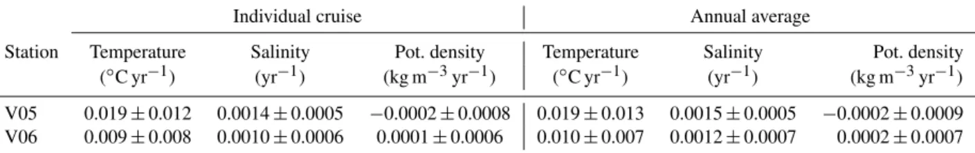
A more holistic picture may be seen by considering the changes of the average hydrographic properties for the over-flow layer at section V as a whole. As before, we define the overflow layer by the criterion σθ=27.8 kg m−3. For each occupation of stations V05 and V06, we have calculated av-erage values for temperature, salinity, and potential density from the depth of this isopycnal to the bottom (extending the deepest CTD measurement to the bottom). We then cal-culated trends for these parameters both for the individual cruises and for annual averages (Table 4). Confirming our previous conclusions, temperature and salinity were found to have increased, but potential density remained unchanged.
The bottom temperature over the FBC sill follows the tem-perature at 800 m on section N in the southern Norwegian Sea (Fig. 1) fairly well (Fig. 8a) and the salinity at 800 m depth on station S08 in the FSC also varies synchronously with the salinity at 800 m depth on section N (Fig. S6b). This indicates that the water around 800 m depth in section N may be an important upstream source for the FBC overflow. From the rather short time series available, it looks as if the tem-perature and salinity variation at 800 m depth on section N is a reduced (by a factor of 10–20) and lagged (5–10 years) response to the Atlantic inflow (Fig. S6).
Longer time series are available at station (Ocean Weather Ship) M at 66◦N and 2◦E, but the properties (especially salinity) at 800 m or 1000 m depth at station M are not simi-lar to those at section N or in the FSC (Fig. S8). The link be-tween the properties of Atlantic inflow and FBC overflow has been addressed by Eldevik et al. (2009) and will not be dis-cussed further here. We only note that a change in the prop-erties of the upstream source waters (e.g., at 800 m depth on section N) is one obvious mechanism for changing the prop-erties of the FBC overflow.
es-Table 4.Linear trends of average properties of the overflow layer (σθ≥27.8 kg m−3)at stations V05 (96 occupations) and V06 (94 occu-pations) through the observational period. The table shows both the trend calculated from individual cruises and the trend calculated from annual averages.
Individual cruise Annual average
Station Temperature Salinity Pot. density Temperature Salinity Pot. density (◦C yr−1) (yr−1) (kg m−3yr−1) (◦C yr−1) (yr−1) (kg m−3yr−1)
V05 0.019±0.012 0.0014±0.0005 −0.0002±0.0008 0.019±0.013 0.0015±0.0005 −0.0002±0.0009 V06 0.009±0.008 0.0010±0.0006 0.0001±0.0006 0.010±0.007 0.0012±0.0007 0.0002±0.0007
timate says that 2 Sv of overflow water should not require many months to pass through this volume. Therefore, this mechanism should be very rapid. Disentangling the relative importance of these two mechanisms is not obvious from the present data set. Regardless of which mechanism dominates, it seems clear, however, that the density change induced by increased temperatures and salinities of the FBC overflow has not been a reduction (Fig. 8b).
4.3 Overflow modification
On its way from the FBC to the deep western boundary cur-rent off the North America coast, the overflow water mixes with ambient water masses so that the resulting modified overflow is warmed by several degrees. This water mass, termed Iceland–Scotland Overflow Water (ISOW), is usually defined by its density: σθ> 27.8 kg m−3 (e.g., Dickson and Brown, 1994; Saunders, 1994, 1996; Fogelqvist et al., 2003; Kanzow and Zenk, 2014).
In the simplest scheme, the overflow warms from close to 0◦C at the sill of the FBC up to ca. 3◦C in the Labrador Sea, which may be explained by entrainment of equal amounts of ambient water, originating from the Atlantic side of the GSR, with temperatures around 6◦C (Hansen et al., 2004). By multivariate analysis of hydrographic, nutrient, and halo-carbon tracer data collected in July–August 1994, Fogelqvist et al. (2003) concluded that the ISOW contained 46 % of en-trained water already in the Iceland Basin. Since additional entrainment may be expected, it has generally been assumed that the ISOW is a fairly equal mixture of original overflow water and water entrained after passing the ridge.
If there is no detrainment of overflow water into the am-bient waters, this implies a doubling of volume transport so that FBC overflow after modification should contribute ap-proximately 4 Sv to the ISOW. This value will, of course, be reduced if there is substantial detrainment.
The water mass transformation is especially intensive in the region immediately downstream of the FBC where the cold overflow meets and entrains the much warmer ambient water from the Atlantic. From their detailed survey, Mau-ritzen et al. (2005) found that “the entrainment is sufficient to cause an approximate doubling of the transport” within 100 km of the sill and they did not find any evidence of
de-trainment. Based on measurements from a series of moored arrays, Geyer et al. (2006) reported that the mixing pro-cesses involved highly periodic oscillations with periods of a few days, which have been further discussed in a number of studies (Darelius et al., 2011, 2013, 2015) and seem to be the manifestation of baroclinic instability (Guo et al., 2014; Darelius et al., 2015).
These studies have done much to clarify the processes that modify the FBC overflow immediately downstream of the channel. Quantifying the effects of entrainment/detrainment on the transport of the modified overflow plume will, how-ever, probably require long-term observations from moored arrays that can determine transport in various density or tem-perature classes. Geyer et al. (2006) did not attempt this, and neither did Darelius et al. (2011), but Ullgren et al. (2016) did present such an attempt. Based on year-long measure-ments on two mooring arrays, they found that detrainment from the overflow plume downstream of the FBC sill was of comparable magnitude to the entrainment and they only measured (1.7±0.7) Sv of “modified overflow” (colder than 6◦C) through their westernmost array 85 km downstream of the sill.
This result indicates that the assumption of substantial transport increase due to entrainment may not be valid and it could even indicate transport decrease. That conclusion would, however, be premature since the westernmost moor-ing array in Ullgren et al. (2016) did not cover the entire plume of overflow water. This is clear from observations of overflow water south of the array (unpublished data; Faroe Marine Research Institute). Unfortunately, the observational evidence is not sufficient to allow for a quantitative revision of the results of Ullgren et al. (2016).
the original 1.9 Sv of FBC overflow denser than 27.8 kg m−3 (HØ2007).
Less dense (σθ< 27.8 kg m−3) components of modified FBC overflow may, however, also contribute to the AMOC, e.g., through entrainment into the DS overflow. For the meridional overturning circulation across a section along 59.5◦N (southern tip of Greenland), Sarafanov et al. (2012) found the boundary between the upper (northward flow-ing) and deeper (southward flowflow-ing) branches to be at
σθ =27.55 kg m−3. This could help explain how both Dick-son and Brown (1994) and Sarafanov et al. (2012) by quite different methods found a total southward transport of dense (σθ> 27.8 kg m−3) water out of the Iceland and Irminger basins to be more than 13 Sv.
There is also the question of whether the mooring ar-rays over the northern slope of the Iceland Basin (Saunders, 1996; Kanzow and Zenk, 2014) cover the entire ISOW trans-port. Certainly, CFC-11 inventories presented by Smethie and Fine (2001) indicated much higher ISOW production rates and an updated estimate by LeBel et al. (2008) included 5.7 Sv of ISOW with 55 % being entrained water. This was for the 1970–1997 period, i.e., before our observations, but Olsen et al. (2008) do not find the Iceland–Scotland overflow to have weakened since 1970.
To some extent, this discrepancy may be caused by the highly variable overflow component at the very depths of the Iceland Basin (de Boer et al., 1998). According to van Aken (2000), ISOW in the Iceland Basin is found below the lower deep water, which partly derives from Antarctic Bot-tom Water (AABW). This is supported by the botBot-tom-near oxygen maximum shown by Sarafanov et al. (2012; their Fig. 5c), but apparently the mooring arrays (Saunders, 1996; Kanzow and Zenk, 2014) have not covered this flow ade-quately.
This is also linked to the further pathways of ISOW. Orig-inally, it was thought that the ISOW had to flow through the Charlie–Gibbs Fracture Zone in order to pass from the Eastern to the Western basins (Dickson and Brown, 1994), but Saunders (1994) only found (2.4±0.5) Sv of ISOW (σθ> 27.8 kg m−3)to follow this path. Based on float trajec-tories, Kanzow and Zenk (2014) showed, however, that there are alternative paths.
In addition to this, part of the ISOW continues southwards in the Eastern Basin and may be traced all the way to the Madeira Abyssal Plain (van Aken, 2001). LeBel et al. (2008) estimated that as much as one-third of the ISOW may take this pathway.
Summarizing, the contribution of modified FBC overflow and Iceland–Scotland overflow as a whole to NADW and AMOC seems still not to be well quantified. According to some estimates, entrainment of water from the Atlantic side of the GSR more than doubles the volume transport, whereas other studies indicate much smaller transports.
4.4 FBC overflow and AMOC
Whereas a weakened AMOC is usually associated with re-duced heat transport, our results show that the FBC overflow in fact experienced stable volume transport and increasing temperature, which implies increasing heat transport. If we assume that the whole overflow layer warmed by a bit more than 0.1◦C after 2002 (Fig. 4b and Table 4), the increase in heat transport is≈1 TW (1012W). To put this into perspec-tive, Purkey and Johnson (2010) suggested a warming rate of (35±31) TW for the whole water column below 2000 m depth, globally, between the 1990s and 2000s. The impli-cations of this depend on two questions: (1) how much of the FBC overflow ends below 2000 m and (2) how much At-lantic water (which has also warmed) does it entrain en route. Both of these are still open questions, as argued, and they are important for assessing the role of the FBC overflow in the global energy budget.
We now return to the question raised in the introduction. How do our observations of a stable FBC overflow since 1995 fit with the claim by Smeed et al. (2014) of a significant weakening from 2004 to 2012 of the transport through the RAPID array (www.rapid.ac.uk/) at 26◦N of lower NADW (LNADW), which they consider to be fed by the overflows?
The FBC overflow is, of course, just one overflow compo-nent, accounting for only ca. one-third of the total overflow, but the other main component, the DS overflow, has also been reported to have no significant trend in transport (Jochumsen et al., 2012, 2015). A substantial reduction in total overflow would also require compensation in some other component of the Arctic Mediterranean water balance. The main inflow to this region is the Atlantic inflow to the Nordic seas, which has three branches. All of these have been monitored since the mid-1990s and none of them show any sign of weakening (Jónsson and Valdimarsson, 2012; Hansen et al., 2015b; Berx et al., 2013) while the inflow from the Pacific has increased from 2001 to 2011 (Woodgate, 2012). A weakening of the to-tal overflow might conceivably be compensated by increased outflow in some other branch, such as the low salinity flow over the East Greenland Shelf, which is badly constrained by observations. Such a hypothetical increase would, however, have to be relatively high since the total overflow is the main outflow from the Arctic Mediterranean.
Smeed et al. (2014) suggested a possible explanation in-volving increased storage of LNADW north of the RAPID array during the period of reduced LNADW flow associated with an uplift of isolines. Another possibility would be a strong reduction in the entrainment of waters from the At-lantic into the overflows, but that would be pure conjecture.
ocean, isolines must slope and cross depth levels. To link the LNADW weakening through RAPID to weakened over-flow contribution requires verification that the boundaries between the various components of NADW and between NADW and AABW across the Atlantic have not moved sub-stantially during the RAPID period.
Whatever the reason for the discrepancy between the RAPID and the overflow measurements, our results clearly indicate that the FBC overflow has remained stable in vol-ume transport and in density since the mid-1990s. Thus, our results are consistent with the general picture of stable ex-changes across the GSR during the last 2 decades and no weakening of the northernmost extension of the AMOC.
5 Data availability
Most of the data used in this study are available online at www.envofar.fo/index.php?page=climate.
The Supplement related to this article is available online at doi:10.5194/os-12-1205-2016-supplement.
Competing interests. The authors declare that they have no conflict
of interest.
Acknowledgements. The authors wish to thank captains and crew
on the RV Magnus Heinason as well as Regin Kristiansen for unfailing support during measurements at sea, and Ebba Mortensen for data processing. Funding for the in situ measurements has been obtained from the Environmental Research Programme of the Nordic Council of Ministers (NMR) 1993–1998, from national Nordic research councils, from the Danish DANCEA programme, and from the European Framework Programs, lately under grant agreement no. GA212643 (THOR) and under grant agreement no. 308299 (NACLIM). Analysis and preparation of this manuscript was mainly funded by the NACLIM project. We thank three anonymous referees for very constructive comments.
Edited by: M. Hoppema
Reviewed by: three anonymous referees
References
Beaird, N. L., Rhines, P. B., and Eriksen, C. C.: Overflow waters at the Iceland-Faroe Ridge observed in multiyear Seaglider sur-veys, J. Phys. Oceanogr., 43, 2334–2351, doi:10.1175/JPO-D-13-029.1, 2013.
Berx, B., Hansen, B., Østerhus, S., Larsen, K. M., Sherwin, T., and Jochumsen, K.: Combining in situ measurements and altimetry to estimate volume, heat and salt transport variability through the Farœ-Shetland Channel, Ocean Sci., 9, 639–654, doi:10.5194/os-9-639-2013, 2013.
Borenäs, K. M. and Lundberg, P. A.: On the deep-water flow through the Faroe Bank Channel, J. Geophys. Res., 93, 1281– 1292, 1988.
Borenäs, K. and Lundberg, P.: The Faroe-Bank Channel deep-water overflow, Deep-Sea Res. Pt. II, 51, 335–350, 2004.
Borenäs, K. M., Lake, I. M., and Lundberg, P. A.: On the interme-diate water masses of the Faroe-Bank Channel overflow, J. Phys. Oceanogr., 31, 1904–1914, 2001.
Collins, M., Knutti, R., Arblaster, J., Dufresne, J.-L., Fichefet, T., Friedlingstein, P., Gao, X., Gutowski, W. J., Johns, T., Krinner, G., Shongwe, N., Tebaldi, C.,Weaver, A. J., and Wehner, M.: Long-term climate change: projections, commitments and irre-versibility, Chap. 12, in: Climate Change 2013: the Physical Sci-ence Basis. Contribution ofWorking Group I to the Fifth Assess-ment Report of the IntergovernAssess-mental Panel on Climate Change, edited by: Stocker, T. F., Qin, D., Plattner, G.-K., Tignor, M., Allen, S. K., Boschung, J., Nauels, A., Xia, Y., Bex, V., and Midgley, P. M., Cambridge University Press, Cambridge, UK, New York, NY, USA, 2013.
Darelius, E., Fer, I., and Quadfasel, D.: Faroe Bank Channel over-flow: mesoscale variability, J. Phys. Oceanogr., 41, 2137–2154, doi:10.1175/JPO-D-11-035.1, 2011.
Darelius, E., Ullgren, J. E., and Fer, I.: Observations of barotropic oscillations and their influence on mixing in the Faroe Bank Channel overflow region, J. Phys. Oceanogr., 43, 1525–1532, doi:10.1175/JPO-D-13-059.1, 2013.
Darelius, E., Fer, I., Rasmussen, T., Guo, C., and Larsen, K. M. H.: On the modulation of the periodicity of the Faroe Bank Channel overflow instabilities, Ocean Sci., 11, 855–871, doi:10.5194/os-11-855-2015, 2015.
De Boer, C. J., van Aken, H. M., and van Bennekom, A. J. : Hy-drographic variability of the overflow water in the Iceland Basin, ICES Coop. Res. Rep., 225, 136–149, 1998.
Dickson, R. R. and Brown, J.: The production of North Atlantic deep water, sources, rates, and pathways, J. Geophys. Res., 99, 12319–12341, doi:10.1029/94JC00530, 1994.
Eldevik, T., Nilsen, J. E. Ø., Iovino, D., Olsson, K. A., Sandø, A. B., and Drange, H.: Observed sources and variability of Nordic seas overflow, Nat. Geosci., 2, 406–410, doi:10.1038/ngeo518, 2009. Fogelqvist, E., Blindheim, J., Tanhua, T., Østerhus, S., Buch, E., and Rey, F.: Greenland-Scotland overflow studied by hydro-chemical multivariate analysis, Deep-Sea Res. Pt. I, 50, 73–102, 2003. Geyer, F., Østerhus, S., Hansen, B., and Quadfasel, D.: Observations
of highly regular oscillations in the overflow plume downstream of the Faroe Bank Channel, J. Geophys. Res., 111, C12020, doi:10.1029/2006JC003693, 2006.
Griesel, A. and Maqueda, M. A. M.: The relation of meridional pressure gradients to North Atlantic Deep Water volume trans-port in an ocean general circulation model, Clim. Dynam., 26, 781–799, doi:10.1007/s00382-006-0122-z, 2006.
Guo, C., Ilicak, M., Fer, I., Darelius, E., and Bentsen, M.: Baroclinic instability of the Faroe Bank Channel overflow, J. Phys. Oceanogr., 44, 2698–2717, doi:10.1175/JPO-D-14-0080.1, 2014.
Hansen, B. and Østerhus, S.: North Atlantic–Nordic Seas ex-changes, Prog. Oceanogr., 45, 109–208, 2000.
Hansen, B., Turrell, W. R., and Østerhus, S.: Decreasing overflow from the Nordic seas into the Atlantic Ocean through the Faroe Bank channel since 1950, Nature, 411, 927–930, 2001. Hansen, B., Østerhus, S., Quadfasel, D., and Turrell, W.: Already
the day after tomorrow?, Science, 305, 953–954, 2004. Hansen, B., Hátún, H., Kristiansen, R., Olsen, S. M., and
Øster-hus, S.: Stability and forcing of the Iceland-Faroe inflow of water, heat, and salt to the Arctic, Ocean Sci., 6, 1013–1026, doi:10.5194/os-6-1013-2010, 2010.
Hansen, B., Larsen, K. M. H., Kristiansen, R., Mortensen, E., and Østerhus, S.: Faroe Bank Channel overflow 1995–2015, Havstovan nr.: 15-02, Technical report, http://www.hav.fo/PDF/ Ritgerdir/2015/TecRep1502.pdf, 2015a.
Hansen, B., Larsen, K. M. H., Hátún, H., Kristiansen, R., Mortensen, E., and Østerhus, S.: Transport of volume, heat, and salt towards the Arctic in the Faroe Current 1993–2013, Ocean Sci., 11, 743–757, doi:10.5194/os-11-743-2015, 2015b. Harden, B. E., Pickart, R. S., Valdimarsson, H., Våge, K., de Steur,
L., Richards, C., Bahr, F., Torres, D., Børve, E., Jónsson, S., Macrander, A., Østerhus, S., Håvik, L., and Hattermann, T.: Up-stream sources of the Denmark Strait Overflow: Observations from a high-resolution mooring array, Deep-Sea Res. Pt. I, 112, 94–112, doi:10.1016/j.dsr.2016.02.007, 2016.
Hermann, F.: The TS diagram analysis of the water masses over the Iceland–Faroe Ridge and in the Faroe Bank Channel, Rapp. PV Reun. Cons. Int. Explor. Mer., 157, 139–149, 1967.
Jochumsen, K., Quadfasel, D., Valdimarsson, H., and Jonsson, S.: Variability of the Denmark Strait overflow: moored time se-ries from 1996–2011, J. Geophys. Res.-Oceans, 117, C12003, doi:10.1029/2012JC008244, 2012.
Jochumsen, K., Köllner, M., Quadfasel, D., Dye, S., Rudels, B., and Valdimarsson, H.: On the origin and propaga-tion of Denmark Strait overflow water anomalies in the Irminger Basin, J. Geophys. Res.-Oceans, 120, 1841–1855, doi:10.1002/2014JC010397, 2015.
Jónsson, S. and Valdimarsson, H.: Water mass transport variability to the North Icelandic shelf, 1994–2010, ICES J. Mar. Sci., 69, 809–815, doi:10.1093/icesjms/fss024, 2012.
Kanzow, T. and Zenk, W.: Structure and transport of the Iceland Scotland Overflow plume along the Reykjanes Ridge in the Ice-land Basin, Deep-Sea Res. Pt. I, 86, 82–93, 2014.
Larsen, K. M. H., Hátún, H., Hansen, B., and Kristiansen, R.: At-lantic water in the Faroe area: sources and variability, ICES J. Mar. Sci., 69, 802–808, doi:10.1093/icesjms/fss028, 2012. LeBel, D. A., Smethie, W. M., Rhein, M., Kieke, D., Fine, R. A.,
Bullister, J. L., Min, D.-H., Roether, W., Weiss, R. F., Andrié, C., Smythe-Wright, D., and Jones, E. P.: The formation rate of North Atlantic Deep Water and Eighteen Degree Water calculated from CFC-11 inventories observed during WOCE, Deep-Sea Res. Pt. I, 55, 891–910, doi:10.1016/j.dsr.2008.03.009, 2008.
Mauritzen, C., Price, J., Sanford, T., and Torres, D.: Circulation and mixing in the Faroese Channels, Deep-Sea Res. Pt. I, 52, 883– 913, doi:10.1016/j.dsr.2004.11.018, 2005.
Munk, W. and Wunsch, C.: Abyssal recipes II: energetics of tidal and wind mixing, Deep-Sea Res. Pt. I, 45, 1977–2010, 1998. Olsen, S. M., Hansen, B., Quadfasel, D., and Østerhus, S.:
Ob-served and modelled stability of overflow across the Greenland– Scotland ridge, Nature, 455, 519–522, 2008.
Olsen, S. M., Hansen, B., Østerhus, S., Quadfasel, D., and Valdimarsson, H.: Biased thermohaline exchanges with the Arc-tic across the Iceland-Faroe Ridge in ocean climate models, Ocean Sci., 12, 545–560, doi:10.5194/os-12-545-2016, 2016. Østerhus, S., Sherwin, T., Quadfasel,D., and Hansen, B.: The
over-flow transport east of Iceland, Chap. 18, in: Arctic-Subarctic Ocean Fluxes: Defining the Role of the Northern Seas in Climate, edited by: Dickson, R. R., Meincke, J., and Rhines, P., Springer Science C Business Media B. V., 427–441, 2008.
Purkey, S. G. and Johnson, G. C.: Warming of Global Abyssal and Deep Southern Ocean Waters between the 1990s and 2000s: Contributions to Global Heat and Sea Level Rise Budgets, J. Cli-mate, 23, 6336–6351, doi:10.1175/2010JCLI3682.1, 2010. Rahmstorf, S., Box, J. E., Feulner, G., Mann, M. E., Robinson,
A., Rutherford, S., and Schaffernicht, E. J.: Exceptional twenti-ethcentury slowdown in Atlantic Ocean overturning circulation, Nature Climate Change, 5, 475–480, doi:10.1038/nclimate2554, 2015.
Roberts, C. D., Garry, F. K., and Jackson, L.: A Multimodel Study of Sea Surface Temperature and Subsurface Density Fingerprints of the Atlantic Meridional Overturning Circulation, J. Climate, 26, 9155–9174, doi:10.1175/JCLI-D-12-00762.1, 2013.
Robson, J., Hodson, D., Hawkins, E., and Sutton, R.: Atlantic over-turning in decline?, Nat. Geosci., 7, 2–3, 2014.
Sabine, C. L., Feely, R. A., Gruber, N., Key, R. M., Lee, K., Bullis-ter, J. L., Wanninkhof, R., Wong, C. S., Wallace, D. W. R., Tilbrook, B., Millero, F. J., Peng, T.-H., Kozyr, A., Ono, T., and Rios, A. F.: The oceanic sink for anthropogenic CO2, Science, 305, 367–371, 2004.
Sarafanov, A., Falina, A., Mercier, H., Sokov, A., Lherminier, P., Gourcuff, C., Gladyshev, S., Gaillard, F., and Daniault, N.: Mean full-depth summer circulation and transports at the northern pe-riphery of the Atlantic Ocean in the 2000s, J. Geophys. Res., 117, C01014, doi:10.1029/2011JC007572, 2012.
Saunders, P. M.: Cold outflow from the Faroe Bank Channel, J. Phys. Oceanogr., 20, 29–43, 1990.
Saunders, P. M.: The flux of overflow water through the Charlie-Gibbs Fracture Zone, J. Geophys. Res., 99, 12343–12355, 1994. Saunders, P. M.: The flux of dense cold overflow water southeast of
Iceland, J. Phys. Oceanogr., 26, 85–95, 1996.
Saunders, P. M.: The dense northern overflows, Chap. 5.6, in: Ocean Circulation and Climate, edited by: Siedler, G., Church, J., and Gould, J., Academic Press, London, UK, 401–417, 2001. Smeed, D. A., McCarthy, G. D., Cunningham, S. A.,
Frajka-Williams, E., Rayner, D., Johns, W. E., Meinen, C. S., Baringer, M. O., Moat, B. I., Duchez, A., and Bryden, H. L.: Observed decline of the Atlantic meridional overturning circulation 2004– 2012, Ocean Sci., 10, 29–38, doi:10.5194/os-10-29-2014, 2014. Smethie, W. M. and Fine, R. A.: Rates of North Atlantic deep water formation calculated from chlorofluorocarbon inventories, Deep-Sea Res. Pt. I, 48, 189–215, 2001.
Stommel, H.: Thermohaline convection with two stable regimes of flow, Tellus, 13, 224–230, 1961.
Toggweiler, J. R. and Samuels, B.: On the ocean’s large-scale cir-culation near the limit of no vertical mixing, J. Phys. Oceanogr., 28, 1832–1852, 1998.
measurements, Ocean Sci., 12, 451–470, doi:10.5194/os-12-451-2016, 2016.
van Aken, H. M.: The hydrography of the mid-latitude northeast Atlantic Ocean I: The deep water masses, Deep-Sea Res. Pt. I, 47, 757–788, 2000.