Uncovering the Secrets of Unusual Phase Diagrams:
Applications of Two-Dimensional Wang-Landau Sampling
Shan-Ho Tsaia,b, Fugao Wanga,∗, and D. P. Landaua
aCenter for Simulational Physics, University of Georgia, Athens, GA 30602, USA bEnterprise Information Technology Services, University of Georgia, Athens, GA 30602, USA
Received on 28 September, 2007
We use a two-dimensional Wang-Landau sampling algorithm to calculate the density of states for two discrete spin models and then extract their phase diagrams. The first system is an asymmetric Ising model on a triangular lattice with two- and three-body interactions in an external field. An accurate density of states allows us to locate the critical endpoint accurately in a two-dimensional parameter space. We observe a divergence of the spectator phase boundary and of the temperature derivative of the magnetization coexistence diameter at the critical endpoint in quantitative agreement with theoretical predictions. The second model is aQ-state Potts model in an external fieldH. We map the phase diagram of this model forQ≥8 and observe a first-order phase transition line that starts at theH=0 phase transition point and ends at a critical point(Tc,Hc), which must be located in a two-dimensional parameter space. The critical fieldHc(Q)is positive and increases withQ, in qualitative agreement with previous theoretical predictions.
Keywords: Ising and Potts models; Critical endpoints; Two-dimensional Wang-Landau
I. INTRODUCTION
Conventional Monte Carlo methods[1] generate a canoni-cal distribution at a fixed temperatureT and with other rele-vant parameters, such as the external field H, fixed as well. Through histogram reweighting[2] this canonical distribution can then be extended to a region ofTandHnear the respective values used in the initial simulation. For large system sizes, however, the region inT andHfor which the results can be reweighted is very narrow. Therefore, numerous simulations have to be carried out for different values ofT(andH) in order to locate phase transitions in an arbitrary case. In contrast, the Wang-Landau sampling method estimates the density of states directly and accurately[3–5] and allows determination of most thermodynamical quantities forallvalues ofT andHwitha
singlesimulation. Wang-Landau sampling has proven very
useful and efficient in many different applications, including studies of complex systems with rough energy landscapes.
In this paper we show how the Wang-Landau sampling method can be used to study discrete spin models in two-dimensional parameter spaces. The first model we consider is an asymmetric Ising model on a triangular lattice with two-and three-body interactions in a uniform external field. For a range of coupling parameters[6] this model has a critical endpoint (CE), i.e. a point in the phase diagram where a critical line meets and is truncated by a first-order transition line. The bulk critical exponents are believed[7] to be un-changed at the CE, but this has not been checked beyond phe-nomenological theory and renormalization calculations[8]. In 1990 Fisher and Upton argued that a new universal singu-larity in the first-order phase transition line should arise at a CE[7, 9]. This prediction was confirmed by Fisher and
∗Current address: Intel Corporation, PC1-105, 44235 Nobel Drive, Fremont,
CA 94538
Barbosa’s phenomenological studies for an exactly solvable spherical model[9]. Later, Wilding[10] studied critical end-point behavior in a symmetrical binary fluid mixture using a large scale Monte Carlo simulation with multicanonical[11] and histogram reweighting[2] methods. Wilding predicted and observed a singularity in the derivative of the diameter of the liquid-gas coexistence curve at the CE. He also pro-vided the first numerical evidence of the divergence in the curvature of the spectator phase boundary[10], in accordance with previous theoretical prediction[7, 9]; however, a quanti-tative analysis of singularities at the CE was not carried out because much larger system sizes would have been required. Our current work provides a quantitative test of the theoretical predictions[7, 9, 10] for these two divergences at the CE in an asymmetric model.
The second model that we study with the Wang-Landau sampling method is aQ-state Potts model in the presence of an external fieldH. An accurate estimate of the density of states allows us to map out the phase diagram in the(T,H)
plane and test the theoretical prediction by Goldschmidt[12] that this model exhibits a first-order phase transition line start-ing at theH=0 phase transition point and ending at a critical point(Tc,Hc) withHc(Q)>0. The value of Hc(Q) is pre-dicted to increase withQ.
This paper is organized as follows: Sec.II describes the Wang-Landau sampling method, Sec.III defines the asymmet-ric Ising model and presents its results, and Sec.IV is dedi-cated to the Potts model in an external field. Some concluding remarks are given in Sec.V.
II. WANG-LANDAU SAMPLING
The Hamiltonian of the two models studied in this paper has the form
whereE is an interaction energy term and M is the magne-tization of the system. The density of states g(E,M)is the number of spin configurations with energyE and magnetiza-tionM. To overcome the barriers in bothEandMspaces, we have to perform a two-dimensional (2D) random walk as in the spin glass problem [4].
We provide a succinct description of the sampling method here, and more details can be found elsewhere[3–5]. At the start of the simulation, the density of states is unknown, so we simply setg(E,M) =1 for all possible(E,M). Then we begin a random walk in(E,M)space by choosing a site ran-domly and flipping its spin with a probability proportional to 1/g(E,M). If we denoteA′(E′,M′)and A′′(E′′,M′′)as the points before and after a spin is flipped, respectively, the tran-sition probability fromA′toA′′is:
p(A′→A′′) =min
g(E′,M′) g(E′′,M′′),1
. (2)
If the point A′′(E′′,M′′) is accepted we modify the exist-ing density of states by a modification factor f >1, that is, g(E′′,M′′) → g(E′′,M′′)∗ f, and we update the his-togram hof visited states, that ish(E′′,M′′)→h(E′′,M′′) +
1. If A′′(E′′,M′′) is not accepted, we update g(E′,M′)→ g(E′,M′)∗f andh(E′,M′)→h(E′,M′) +1.
We continue performing the random walk until the his-togram h(E,M)is “flat” in(E,M)space. The modification factor f introduces a systematic error whose magnitude for ln[g(E,M)]is proportional to ln(f). To reduce this source of error, we systematically reduce the modification factor using a function like fi+1=fi1/n(n>1) whereihere denotes the level of iteration in the algorithm (in each iteration a separate 2D random walk is performed in (E,M)space). To be ex-plicit, when iterationigenerates a “flat” histogram, we reset the histogram to zero, and begin the next iteration with a new factor fi+1and the lastg(E,M)as the starting value. We end
the simulation when the modification factor is smaller than a predefined value (such as lnffinal=10−8used in Sec.III and
10−6 used in Sec.IV). To speed up the convergence of the
density of states to the true value, the initial modification fac-tor was as large as f =f0=e≃2.71828..., andn=4 in our
simulations.
We should point out that it is impossible to obtain a per-fectly flat histogram. In this work the histogram is considered “flat” when the number of entries larger than or equal to 2000 remains unchanged forL2×106spin flip trials. For small
lat-tices (up toL=24) our tests showed that the results so ob-tained agree well with those found when using a more strin-gent flatness criterion, namely the histogram is considered “flat” when h(E,M) for all possible (E,M)is not less than 80% of the average histogramh(E,M). For large lattices we may need to divide the two-dimensional parameter space into regions and perform separate random walks[3, 4, 13], because with our current computational resources it is very difficult to obtain a flat histogram for a single random walk over the en-tire(E,M)parameter space. However, problems arise from different choices of the parameter space decomposition, as we will discuss in Sec.IV.
With an accurate estimate of the density of statesg(E,M), we can calculate thermodynamic quantities at any temperature T, and external magnetic fieldHfor the system with Hamil-tonian given in Eq.(1).
A mathematical proof of the convergence of the Wang-Landau method was given by Zhou and Bhatt [14] and ap-plications of this method already include simulations of flu-ids [15] (continuum systems), protein folding [16], polymer films [17], polymer collapse [18–20], binary Lennard-Jones glass [21], liquid crystals [22], random spin systems [23, 24], atomic clusters [25], optimization problems [26], combina-torial number theory [27], Blume-Capel model [28], and 3D Potts model [29, 30]. This method has been improved by using N-fold way [31] and multibondic sampling [32, 33], and it also has been generalized to perform quantum Monte Carlo simulations [34, 35] and sampling along the reaction coordinates for a molecular system [36]. By suitable adapta-tion of the problem, multidimensional numerical integraadapta-tion has also been successfully treated using Wang-landau sam-pling [37]. A rigorous derivation for off-lattice implementa-tion of this algorithm was given in Ref. 38. Further general-izations and studies of this sampling technique have also been carried out [13, 39–44].
III. ASYMMETRIC ISING MODEL
The model considered here is described by the Hamiltonian
H
=−J∑
i j
SiSj−J3
∑
i jk
SiSjSk−H
∑
iSi (3)
whereSi=±1 is an Ising spin on siteiof a triangular lattice with linear size L, i jdenotes nearest-neighbor spin-pairs, andi jkrepresents the three spins on the elementary trian-gles. The parametersJandJ3are two- and three-body
nearest-neighbor spin couplings, respectively, and H is an external field. Previous Monte Carlo simulations by Chin and Lan-dau [6] showed that this model exhibits critical endpoints for a range of values ofJandJ3. In particular, forJ=1 andJ3=2
(parameters used here) there is a CE that is well-separated from a critical point at the end of the first-order phase tran-sition line.
We use Wang-Landau sampling[3–5] described in Sec.II withE =∑i jSiSj+2∑i jkSiSjSk andM=∑iSi to deter-mine the density of states g(E,M), and from it we obtain thermodynamical quantities such as the magnetization, spe-cific heat, susceptibility, order parameter[45, 46], etc. Mul-tiple, independent random walks were performed to look for unexpected behavior resulting from different random number streams as well as to allow the determination of error bars.
-6 -5 -4 -3 -2 -1 H 0 1 2 3 4 5 6 7 8 T -2.96 -2.94 H 2.4 2.44 2.48 T L=30 L=42 L=∞ L=∞ (T,H)CE
Tc(H) Hσ(T)
B(- - -)
C(- - +) A(+ + +) (T,H)c
(T,H)CE
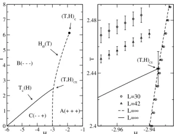
FIG. 1: (left) Phase diagram in the (T,H) plane extrapolated to
L=∞. For finiteL, the phase boundaries were determined by the locations of the maximum of the susceptibility. The solid line is a critical line and the dashed line is a first-order phase transition line. The figure on the right shows the region near the critical endpoint and includes data forL=30 (circles) andL=42 (triangles) to illustrate the finite-size effects.
and a ferrimagnetic phase C(- - +) withM(0,H) =−1/3 (the spins on two sublattices are down and on the other are up).
The critical endpoint for L = ∞ is estimated as
(T,H)CE = (2.443(10),−2.934(10))and the Ising-like crit-ical point at the end of the first-order line is at (T,H)c=
(6.125(3),−1.879(2)). Our tests[45, 46] showed that the critical line Tc(H)for this asymmetric Ising model is in the same universality class as the two-dimensional Q=3 Potts model[47], as expected due to symmetry considerations. We recall that the conjectured values[47] for the critical exponents of the 2DQ=3 Potts model areα=1/3,β=1/9,γ=13/9, andν=5/6.
In Fig.2(left), the curvatures d2Hσ(T)/dT2of the specta-tor phase boundary show a very clear singularity at the CE. According to a general finite-size scaling argument [7, 10], this curvature should diverge at the CE with a specific heat-like form
d2Hσ(T,L) dT2
CE
= a0+a1Lα/ν, (4)
whereα andνare critical exponents defined on the critical line Tc(H) and a0 is a background. Using the conjectured
exponents for the 2D Q=3 Potts model[47], the predicted scaling exponent (see Eq. (4)) isα/ν=2/5.
Figure 2(right) shows a plot of the maximum ofd2Hσ/dT2, denoted as f(L), as a function ofLα/ν=L0.4. The scaling re-lation is obtained by a linear fit to the data forL=18 to 42 to Eq. (4), witha0anda1as fitting parameters and with the
ex-ponent fixed atα/ν=2/5=0.4. Because we obtained quite a good fit to the scaling function f(L) =a0+a1L0.4[solid line
in Fig. 2(right)] we can conclude that our data are in good agreement with the predicted scaling exponent (see Eq. (4)), but the background term is not negligible. Our data also
in-2 2.5 3
T 0.1 0.2 0.3 0.4 d 2 H σ /dT 2
2 3 4 5
Lα/ν 0.1
0.2 0.3 0.4
maximum of d
2 H
σ
/dT
2 = f(L)
f(L) = a0+a1 Lα/ν L=42
L=36
L=30
L=21
L=15
a1 = 0.106(8) a0 = -0.11(3)
α/ν=2/5=0.4
FIG. 2: (left) Singularity of the curvatured2Hσ/dT2of the spectator phase boundaryHσand (right) the finite-size scaling of the maximum of this curvature, which we denote f(L), versusLα/ν=L0.4. For clarity, in (left) we only show a few of the larger error bars forL=42. (Other error bars are smaller, particularly away from the peaks.) The solid line in (right) is a linear fitting of the data.
2 2.5 3
T 1.2 0.8 0.4 0 -0.4 -dM d /dT
|Hσ
10 20 30 40
0 L 0.2 0.4 0.6 0.8 1.0 1.2
maximum of -dM
d /dT = ζ (L) L=42 L=36 L=30 L=21 L=15
ζ(L)=c0+c1 Lα/ν+ c2 L(1-β)/ν
α/ν=0.4 (1-β)/ν=1.07
FIG. 3: (left)Singularity of the derivative of the magnetization co-existence diameter−dMd/dT alongHσ and (right) the finite-size scaling of the maximum of this derivative. For clarity, in (left) we only show a few of the larger error bars forL=42. (Other error bars are smaller, particularly away from the peaks.)
dicate that there are small correction terms to the finite-size scaling; however, the resolution of our data and the lattice sizes used here are not adequate to estimate these correction terms.
The magnetization coexistence diameterMd is defined as
the average magnetization along the first-order transition line Hσ(T). Using generalized scaling arguments, Wilding [10] predicted that the coexistence diameter derivative diverges as
dMd(T,H) dT CE
=c0+c1Lα/ν+c2L(1−β)/ν (5)
whereα,β, andνare critical exponents defined on the critical lineTc(H). We observe a clear divergence of the derivative
0.68 0.7 0.72 T
-0.02 0 0.02
H
L = 24
L = 32
L = 48
L =
∞
Q=10 (Tc,Hc)
in state 1
in state 1
disordered Triple point
phase phase rich
phase poor
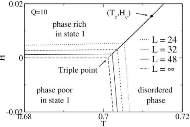
FIG. 4: Phase diagram in the(T,H)plane for theQ=10 ferromag-netic Potts model. For finiteLthe phase transition lines are deter-mined from equal height peaks in the magnetization probability dis-tributionP(M,T,H). The solid circle shows theL=∞critical point, denoted(Tc,Hc). The long-dashed line shows the extrapolation of the phase transition lines toL=∞, and the line segment forH>0 starts atH=0 and ends at(Tc,Hc).
of the maximum of−dMd/dT with lattice sizeL. The solid
line in Fig. 3(right) is a least squares fitting of the maximum of−dMd/dT using Eq. (5) withL=15 to 42 data. For the
symmetric binary fluid studied by Wilding [10], the coeffi-cientc2 in Eq. (5) is predicted to vanish; thereforedMd/dT
should diverge withLα/νat the CE. However, for the asym-metric model studied here, we obtained a better fit whenall
terms in the right-hand side of Eq. (5) were included.
IV. Q-STATE POTTS MODEL IN AN EXTERNAL FIELD
The second model considered here is described by the Hamiltonian
H
=−J∑
i j
δσi,σj−H
∑
i
δσi,1 (6)
where σi =1,2,· · ·Q on site i of a two-dimensional L×L
square lattice, i j denotes pairs of nearest-neighbor spins, J>0 is a ferromagnetic coupling, andHis an external field. We use the Wang-Landau sampling[3–5] described in Sec.II withE=−∑i jδσi,σj andM=∑iδσi,1to determine the
den-sity of states g(E,M)and from it we obtain the energy and magnetization probability distributions at different values of T andH.
Figure 4 shows the phase diagram for the Q=10 Potts model, for lattices withL=24,32,48 and the extrapolation to L=∞using finite size scaling. For finite lattices, three “1st-order” phase boundaries meet at a triple point which occurs for non-zero field; however, this point extrapolates toH=0 in the thermodynamical limit. This means that the “ordinary”, 1st order Potts model transition is actually a triple point. The phase transition lines are determined from equal height peaks in the magnetization probability distributionP(M,T,H). Near the triple point,P(M,T,H)has three peaks, corresponding to (i) a phase rich in state 1, (ii) a phase poor in state 1, and
0 500 1000 1500 2000
M 0
0.001 0.002 0.003 0.004 0.005
P(M,T,H)
H=0.002, T=0.702620 H=0.001, T=0.702251 Q=10, L=48
FIG. 5: Magnetization probability distributionP(M,T,H)forQ=
10,L=48, obtained from the density of statesg(E,M).
4 5 6 7 8 9 10 11
Q
0.00 0.01 0.02
H c
FIG. 6: Critical fieldHcas a function ofQ. The solid line is a guide to the eye and the point atQ=4 is the exact value.
(iii) a disordered state, as illustrated in Fig.5. For each set of parameters(T,H) the right-most peak in Fig.5 corresponds to phase (i), the left-most peak to phase (ii), and the mid-dle peak to (iii). For L=∞we observe a first-order phase transition line starting at theH=0 phase transition point and ending at a critical point(Tc,Hc), shown as a solid circle in
Fig.4. Note that for finite latticesP(M,T,H)continues to have two equal height peaks forH>Hc; however, the logarithm
of the value of the peak height over the value of the mini-mum of the distribution between the two peaks decreases[48] withLforHabove Hc. For eachLthe phase transition line
separating phases (i) and (ii) goes to (T,H) = (0,0). The H=0 phase transition temperature obtained in our simula-tion isTpt=0.701228(10), in good agreement with the exact
resultTptexact=0.701231....
ForQ=8,9 we have also located a first-order phase tran-sition line starting at the respectiveH=0 phase transition points and ending at a critical point. The critical fieldHc(Q)
increases withQ, as shown in Fig.6, in qualitative agreement with previous theoretical predictions[12]. For smallerQthe critical field becomes tiny, and determining its location asQ approaches 4 will be challenging.
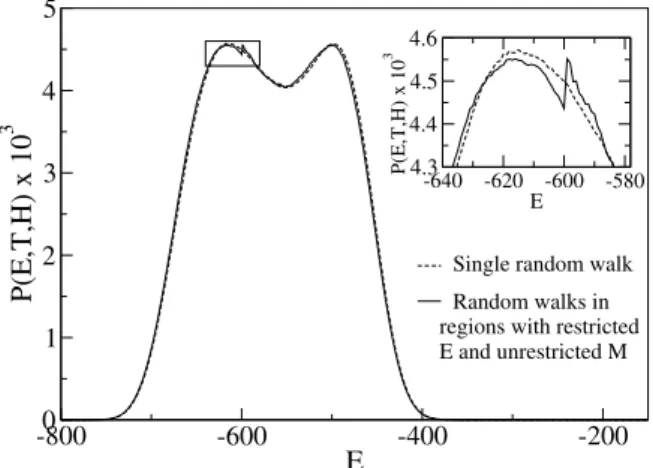
L≤48, and a single random walk in the entire(E,M)space. For smallerQvalues (Q=5,6,7), the finite size effects are stronger and larger lattices are needed in order to locate the critical point accurately. However, with our current computa-tional resources it is very difficult to carry out a single 2D random walk over the entire (E,M) parameter space forL much larger than 48. Parallel, one-dimensional Wang-Landau sampling, in which independent random walks are carried out in restricted phase space regions, has been implemented with success in previous work[3, 4, 13]. Therefore, we have also tried to parallelize the 2D algorithm by performing indepen-dent random walks on overlapping (E,M) regions. We di-vided the parameter space into strips with: (i) restricted val-ues ofEand unrestrictedM, (ii) restrictedMand unrestricted E, and (iii) bothEandMrestricted. The independent random walks were carried out in parallel, and each generated a sity of states for the respective random walk regions. The den-sities of states from two adjacent random walk regions were then normalized with one overlapping(E,M)point. However, we found that the resulting density of states over the entire
(E,M)range had some small discontinuities, which carried over to the probability distributions of energy and magnetiza-tion, as illustrated in Fig.7. For the division in case (i), the
-800 -600 -400 -200
E 0
1 2 3 4 5
P(E,T,H) x 10
3
Single random walk
Random walks in -640 -620 -600 -580
E 4.3
4.4 4.5 4.6
P(E,T,H) x 10
3
regions with restricted E and unrestricted M
FIG. 7: Energy probability distribution for Q=5, L=20, T =
0.85977 andH=0 computed from ag(E,M)obtained with a par-allel two-dimensional random walk, where the independent random-walk regions have restricted values of E and unrestrictedM, as in case (i) in the text. The inset shows an enlarged view of the jump inP(E,T,H), in the region marked by the square box in the main figure.
distributionP(M,T,H)agreed well with the result from a sin-gle random walk over the entire(E,M)space; however, the energy distribution P(E,T,H) had a number of
discontinu-ities. For case (ii),P(E,T,H)was correct, butP(M,T,H)had a number of small jumps. The parallelization in (iii) also gen-erated jumps inP(M,T,H). The general source of these diffi-culties seems to be due to the difficulty in matching surfaces at the boundaries rather than curves as in one-dimensional ran-dom walks. Thus, the simple parallelization described above cannot be used to obtain accurate phase diagrams. In the par-allel Wang-Landau sampling ofg(E)performed in Ref.4 the random walk within each energy region was restarted period-ically from independent spin configurations, to ensure that all spin configurations with energies in the restricted range can be equally accessed. This approach might be helpful too for the parallel Wang-Landau sampling of g(E,M). Another viable simulational approach to study the Q=5,6,7 models is to perform 2D Wang-Landau sampling on systems withL≤48 and use these results to guide more standard hybrid Monte Carlo algorithms for larger lattices at a few values of(T,H).
V. CONCLUSION
We used Wang-Landau sampling with a two-dimensional random walk to determine the density of statesg(E,M)for an asymmetric Ising model with two- and three-body interactions on a triangular lattice, in the presence of an external field. An accurate g(E,M)allowed us to map out the phase diagram accurately and to observe a clear divergence of the spectator phase boundary and of the magnetization coexistence diame-ter derivative at the critical endpoint. The exponents for both divergences agree well with the predicted values[7, 10].
We also applied the 2D Wang-Landau sampling method to obtaing(E,M)for theQ-state ferromagnetic Potts model in the presence of an external field. We mapped out the phase diagram forQ=8,9,10 and observed a first-order phase tran-sition line starting at theH=0 phase transition temperature and ending at a critical point(Tc,Hc)withHc>0. The critical
field increases withQ, in qualitative agreement with previous large-Qseries expansion results[12]. Our attempts to paral-lelize the algorithm demonstrated that further development is needed to avoid subtle errors that arise from the process.
Acknowledgments
We thank K. Binder, H. Meyer, and J. A. Plascak for helpful discussions, and P. Brunk for technical assistance with com-puter resources. Simulations were performed on an Itanium cluster at SDSC and on computer resources at the Research Computing Center at UGA. This work is partially supported by the NSF under Grants DMR-0341874 and DMR-0307082.
[1] D. P. Landau and K. Binder,A Guide to Monte Carlo Meth-ods in Statistical Physics, second edition (Cambridge U. Press, Cambridge, 2005).
[2] A. M. Ferrenberg and R. H. Swendsen, Phys. Rev. Lett.61, 2635 (1988);63, 1195 (1989).
[3] F. Wang and D. P. Landau, Phys. Rev. Lett.86, 2050 (2001). [4] F. Wang and D. P. Landau, Phys. Rev. E.64, 056101 (2001). [5] D. P. Landau and F. Wang, Comput. Phys. Commun.147, 674
(2002); D. P. Landau, S.-H. Tsai, and M. Exler, Amer. J. Phys.
354 (2004).
[6] K. K. Chin and D. P. Landau, Phys. Rev. B36, 275 (1987). [7] M. E. Fisher and P. J. Upton, Phys. Rev. Lett. 65, 2402
(1990);65, 3405 (1990); M. E. Fisher, Physica A 172, 77 (1991).
[8] T. A. L. Ziman, D. J. Amit, G. Grinstein and C. Jayaprakash, Phys. Rev. B25, 319 (1982).
[9] M. E. Fisher and M. C. Barbosa, Phys. Rev. B43, 11177 (1991); M. C. Barbosa and M. E. Fisher, Phys. Rev. B43, 10635 (1991); M. C. Barbosa, Phys. Rev. B45, 5199 (1992).
[10] N. B. Wilding, Phys. Rev. Lett.78, 1488 (1997); Phys. Rev. E
55, 6624 (1997).
[11] B. A. Berg and T. Neuhaus, Phys. Rev. Lett.68, 9 (1992). [12] Y. Y. Goldschmidt, Phys. Rev. B24, 1374 (1981).
[13] B.J. Schulz, K. Binder, M. M¨uller, and D. P. Landau, Phys. Rev. E67, 067102 (2003).
[14] C. Zhou and R. N. Bhatt, Phys. Rev. E72, 025701(R) (2005). [15] Q. Yan, R Faller, and J. J. de Pablo, J. Chem. Phys.116, 8745
(2002); T. S. Jain and J. J. de Pablo, J. Chem. Phys.118, 4226 (2003).
[16] N. Rathore and J. J. de Pablo, J. Chem. Phys.116, 7225 (2002); N. Rathore, T. A. Knotts, and J. J. de Pablo, J. Chem. Phys.118, 4285 (2003).
[17] T. S. Jain and J. J. de Pablo, J. Chem. Phys.116, 7238 (2002). [18] F. Rampf, K. Binder, and W. Paul, J. Polym. Sci. Part B: Polym.
Phys.44, 2542 (2006).
[19] D. F. Parsons and D. R. M. Williams, Phys. Rev. E74, 041804 (2006); J. Chem. Phys.124, 221103 (2006).
[20] D. T. Seaton, S. J. Mitchell, and D. P. Landau, Braz. J. Phys.36, 623 (2006).
[21] R. Faller and J. J. de Pablo, J. Chem. Phys.119, 4405 (2003). [22] E. B. Kim, R. Faller, Q. Yan, N. L. Abbott, and J. J. de Pablo, J.
Chem. Phys.117, 7781 (2002).
[23] Y. Okabe, Y. Tomita, and C. Yamaguchi, Comput. Phys. Com-mun.146, 63 (2002).
[24] Y. Wu and J. Machta, Phys. Rev. B74, 064418 (2006). [25] F. Calvo and P. Parneix, J. Chem. Phys.119, 256 (2003). [26] M. A. de Menezes and A. R. Lima, Phys. A323, 428 (2003). [27] V. Mustonen and R. Rajesh, J. Phys. A36, 6651 (2003).
[28] C. J. Silva, A. A. Caparica, and J. A. Plascak, Phys. Rev. E73, 036702 (2006).
[29] C. Yamaguchi and Y. Okabe, J. Phys. A.34, 8781 (2001). [30] Y. Okabe and H. Otsuka, J. Phys. A39, 9093 (2006).
[31] B. J. Schulz, K. Binder, and M. M ¨uller, Int. J. Mod. Phys. C13, 477 (2002).
[32] C. Yamaguchi and N. Kawashima, Phys. Rev E65, 056710 (2002).
[33] B. A. Berg and W. Janke, Phys. Rev. Lett.98, 040602 (2007). [34] M. Troyer, S. Wessel, and F. Alet, Phys. Rev. Lett.90, 120201
(2003).
[35] P. N. Vorontsov-Velyaminov and A. P. Lyubartsev, J. Phys. A
36, 685 (2003).
[36] F. Calvo, Mol. Phys.100, 3421 (2002).
[37] Y. W. Li, T. W¨ust, D. P. Landau, and H. Q. Lin, Comput. Phys. Commun.177, 524 (2007).
[38] M. S. Shell, P. G. Debenedetti, and A. Z. Panagiotopoulos, Phys. Rev. E66, 056703 (2002).
[39] Q. Yan and J. J. de Pablo, Phys. Rev. Lett.90, 035701 (2003). [40] N. Rathore, Q. Yan, and J. J. de Pablo, J. Chem. Phys.120, 5781
(2004).
[41] E. A. Mastny and J. J. de Pablo, J. Chem. Phys.122, 124109 (2005).
[42] A. Malakis, A. Peratzakis, and N. G. Fytas, Phys. Rev. E70, 066128 (2004); A. Malakis, S. S. Martinos, I. A. Hadjiaga-piou, N. G. Fytas, and P. Kalozoumis, Phys. Rev. E72, 066120 (2005); A. Malakis and N. G. Fytas, Phys. Rev. E73, 056114 (2006);73, 016109 (2006).
[43] C. Zhou, T. C. Schulthess, S. Torbr¨ugge, and D. P. Landau, Phys. Rev. Lett.96, 120201 (2006).
[44] H. K. Lee, Y. Okabe, and D. P. Landau, Comput. Phys. Com-mun.175, 36 (2006).
[45] S.-H. Tsai, F. Wang, and D. P. Landau, Braz. J. Phys.36, 635 (2006).
[46] S.-H. Tsai, F. Wang, and D. P. Landau, Phys. Rev. E75, 061108 (2007).
[47] F. Y. Wu, Rev. Mod. Phys.54, 235 (1982).