Tese apresentada à Universidade Federal de Viçosa, como parte das exigências do Programa de Pós%Graduação em Meteorologia Agrícola, para obtenção do título de Doctor Scientiae.
VIÇOSA
SANTIAGO VIANNA CUADRA
Tese apresentada à Unive de Viçosa, como parte das Programa de Pós%Graduação e Agrícola, para obtenção do tí Scientiae.
A Deus, pela vida e pelo amor.
À minha esposa Ana Paula Gomes Cuzziol e à minha filha Maria Luiza Cuzziol Cuadra. À minha mãe Denise Vianna e ao meu pai José Lopez.
À minha sogra Virgínia Maria Gomes Carllini.
À Universidade Federal de Viçosa e ao Departamento de Engenharia Agrícola, pela oportunidade de realização do curso.
LISTA DE ABREVIATURAS... vii
LISTA DE SÍMBOLOS ... viii
RESUMO ... ix
ABSTRACT ... xi
1. INTRODUCTION ... 1
2. METHODOLOGY ... 8
2.1. Model description ... 8
2.1.1. Biogeophysical processes represented in Agro%IBIS ... 8
2.1.2. Crop management ... 11
2.1.3. Phenology and carbon allocation ... 14
2.2. Validations and input data sets ... 17
2.2.1. São Paulo state experimental site ... 17
2.2.2. Kalamia estate experimental site ... 18
2.2.3. São Paulo mesoregions ... 19
2.2.4. Louisiana state ... 21
3. RESULTS AND DISCUSSION ... 22
3.1. São Paulo state experimental site ... 22
3.1.1. Leaves biomass and radiation fluxes ... 22
3.1.2. Carbon balance and evapotranspiration ... 28
3.1.3. Energy balance ... 38
3.3. São Paulo mesoregions ... 47
3.4. Louisiana state ... 52
3.5. Relative bias ... 55
4. SUMMARY AND CONCLUSIONS ... 57
APAR – Absorbed Photosynthetic Active Radiation. DAR – Days After Ratooning.
GCM – Global Climate Model. GDD – Growing Degree Days.
IBGE – Brazilian Institute of Geography and Statistics. IBIS – Integrated Biosphere Simulator.
LAI – Leaf Area Index.
Ag – Gross photosynthesis rate. ARs – Absorbed solar radiation.
β – Bowen ratio.
ET – Evapotranspiration.
ET0 – Reference evapotranspiration. FRW – Furrow irrigated.
G – Soil heat flux.
H – Relative humidity.
H – Sensible heat flux.
Ke – Radiation extinction coefficient. λE – Latent heat flux.
RM – Crop relative maturity.
Rn – Net radiation.
Rp – Photosynthetic active radiation flux.
Rs – Solar radiation flux.
CUADRA, Santiago Vianna, D.Sc., Universidade Federal de Viçosa, novembro de 2010. ! " # " $ %& ' " '( ' ! ") ') ) " )*+')( ,)() !#" - $) . Orientador: Marcos Heil Costa. Coorientadores: Aristides Ribeiro e Rosmeri Porfírio da Rocha.
CUADRA, Santiago Vianna, D.Sc., Universidade Federal de Viçosa, November, 2010. $ ,./ ') #-)(') -( 0!. " % ( - $) !#" . Adviser: Marcos Heil Costa. Co%advisers: Aristides Ribeiro and Rosmeri Porfírio da Rocha.
12
The environmental and social impacts of global climate change are one of the greatest challenges facing the human race. Anthropogenic greenhouse gas emissions and land use change (FORSTER et al., 2007; HOUGHTON, 2007; RAMANKUTTY et al., 2008; RAUPACH et al., 2007) are projected to alter the global climate in the next decades (MEEHL et al., 2007). For example, global temperature, precipitation intensity, number of dry days and heat waves are projected to increase and frost days are projected to decrease as result of anthropogenic activities (MEEHL et al., 2007). These changes are expected to have a large impact on both natural and agricultural ecosystems (e.g., COSTA; FOLEY, 2000; MILES et al., 2004; WANG, 2005).
potential to greatly influence biogeochemical and biogeophysical processes across the world (e.g., BETTS et al., 2007; COSTA; FOLEY, 2000; HOUGHTON, 2007; PIELKE et al., 1998).
Many studies have highlighted the potential impact of climate change on agriculture and food security (e.g., CHALLINOR et al., 2007; HAIM et al., 2008; TUBIELLO et al., 2007), particularly in developing regions (EASTERLING et al., 2007). Currently, the most frequently used approach to evaluate these impacts is to use crop models that are then forced by the data from Global Climate Model (GCM) projections. However, this approach suffers from a number of inherent limitations. First, most current global climate models work on a scale of tens to hundreds of kilometers (RANDALL et al., 2007), while crop models are usually developed and validated at the site scale (e.g., DUBROVSKY et al., 2000b). Such spatial scale issues are often not considered (e.g., ALEXANDROV; HOOGENBOOM, 2000) or a statistical or dynamical downscaling technique is applied to bridge this difference (e.g., MEARNS et al., 2001).
Another frequently overlooked issue is the fact that crop development is affected not only by the mean atmospheric conditions, but also by the frequency of extreme events such as frost, heat waves, floods, and droughts (e.g., BAIGORRIA et al., 2007; DUBROVSKY et al., 2000a). Many studies have only included mean climatic changes (usually only temperature and precipitation), and considered the present observed climatic variables statistical distribution (e.g., ALEXANDROV; HOOGENBOOM, 2000; FELKNER et al., 2009). In a few cases this limitation was addressed through a stochastic weather generator with modified parameters based on GCMs simulations (e.g., DUBROVSKY et al., 2000b; HAIM et al., 2008).
Land use change can influence the global climate in at least two ways: Firstly, through alterations in biogeochemical processes – usually releasing CO2 and reducing the capacity of the ecosystem to absorb part of anthropogenic emitted CO2 (HOUGHTON; HACKLER, 2002; HOUGHTON, 2007). Secondly, by changing the physical properties of the land surface (e.g., BETTS et al., 2007; COSTA; FOLEY, 2000; COSTA; YANAGI, 2006; SNYDER; FOLEY, 2004) thereby altering the energy, mass and momentum balances at surface (PIELKE et al., 1998). For example, the replacement of natural forest by grassland or cropland usually alters the latent and sensible heat fluxes at the surface due to the biophysical differences that characterize these vegetation types – e.g. leaf area index, phenology, stomatal conductance, and root profile (LIU, 2003; SOUZA%FILHO et al., 2005; JUAREZ et al., 2007; TWINE et al., 2004).
Most published studies on the biogeophysical impacts of land use change on climate and ecosystems have focused on the replacement of natural vegetation by pasture land (e.g., COE et al., 2009; COSTA; FOLEY, 2000; NOBRE et al., 1991). However, the biophysical differences between pasture and cropland may result in significantly different interactions with the atmosphere (COSTA et al., 2007). For example, crops usually show a higher seasonal variation in land cover faction (e.g. fallow soil period) and in canopy structure (e.g. leaf area index) than pasture, reflected in more pronounced energy and water surface balance differences across the year as compared to the original forest cover.
Recently, there has been an increasing effort to explicitly represent crops in LSMs (e.g. BONDEAU et al., 2007; GERVOIS et al., 2004; KOTHAVALA et al., 2005; KUCHARIK; BRYE, 2003; LOKUPITIYA et al., 2009; OSBORNE et al., 2007). Diverse approaches have been used to incorporate different crop types within LSMs – with crop types varying from a single generic variety (e.g., OLESON et al., 2007) to thirteen crop classes (BONDEAU et al. 2007). The inherent scale flexibility of Agro%LSMs has lead to their successful application at a range of spatial scales: (i) site level (e.g., BONDEAU et al. 2007; GERVOIS et al., 2004; KOTHAVALA et al., 2005; KUCHARIK AND TWINE, 2007; LOKUPITIYA et al., 2009); (ii) regional level (e.g., KUCHARIK, 2003); (iii) global scale (e.g., BONDEAU et al. 2007; OSBORNE et al., 2007).
Representation of crop growth vary between Agro%LSMs, spanning from: (i) few crop characteristics specifications, (ii) coupling LSM and crop models; and (iii) explicit inclusion of crop growth as function of net crop carbon balance. For example, the Canadian LSM (CLASS) pre%specifies the above ground biomass and empirically calculates LAI based on growing degree days (GDD) and longitude (KOTHAVALA et al., 2005). Gervois et al. (2004) coupled the LSM ORCHIDEE (Organizing Carbon and Hydrology in Dynamic Ecosystems) with the crop model STICS (Simulateur Multidisciplinaire pour les Cultures Standard) – and both models are run synchronically and forced with
the same atmospheric conditions, and STICS updates ORCHIDEE with LAI, root density profile, nitrogen stress, and vegetation height. In another example, Osborne et al. (2007) incorporated some of the crop model GLAM (General Large%Area Model for annual crops) functions within the LSM MOSES (Met Office Surface Exchange Scheme). Finally, Agro%IBIS (KUCHARIK, 2003), SiBcrop (LOKUPITIYA et al., 2009) and Agro%BGC (DI VITTORIO et al., 2010) incorporates crops phenologic and physiologic characteristics based on previous crop models and literature review. In such approach, crop growth is dependent on net carbon balance – the same vegetation growth principles applied to the natural ecosystems.
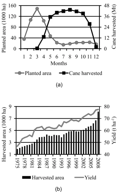
al., 2007). For example, in North America maize has only one crop cycle per year (and may be rotated with typical winter crop such as winter wheat) while in Brazil the common practice is to reap two maize crops per year, in some cases sharing the land with a third crop during the year. This difference determines, for instance, the sowing dates, which is a critical parameter to adequately simulate crop development and its interaction with atmosphere. For regions with marked climatic restrictions on crop growth (e.g., low winter temperatures or a marked dry season) climatic conditions may be a good proxy for sowing dates. However, these are frequently hard to accurately predict as they vary with climatic conditions, biophysical/physiological crop characteristics and management or technological level (e.g., SACKS et al., 2010). Sowing and harvest dates may therefore have a large degree of variability and independence from climatic conditions even in the same region (illustrated in Figure 1). Thus, the derivation of observed global data sets and the simulation of management practices is one of the main challenges when running Agro% LSMs on the global scale (OSBORNE et al., 2007).
Another important challenge in creating a realistic Agro%LSM is how to control the climate model biases when the models are coupled. For instance, at a regional scale climate models may deviate significantly from observations (e.g., DAI, 2006) and affect crop yield. Therefore, climate model biases need to be interactively corrected or considered when crop yield is directly assessed from Agro%LSM coupled simulations (OSBORNE et al., 2007).
(a)
(b)
Source: Based on IBGE statistics (see text).
Figure 1 – São Paulo state (Brazil) monthly sugarcane planted area (thousands of hectares – k ha) and harvested cane (millions of tons – Mt) for the 2007%08 crop season (a); Brazilian sugarcane harvest area (millions of hectares) and average yield (t ha%1) (b).
0 12 24 36 48 0 40 80 120 160
1 2 3 4 5 6 7 8 9 10 11 12
C ane ha rve st ed (M t) P la nt ed ar ea ( 1000 ha ) Months
Planted area Cane harvested
40 50 60 70 80 1 3 5 7 9
1975 1978 1981 1984 1987 1990 1993 1996 1999 2002 2005 2008
Y ie ld (t ha 1 ) H ar ve st ed a re a (1000 ha )
The potential of Agro%LSMs to provide more realistic simulations of yield and to simulate land use or management impacts on local to regional climate has led to increasing efforts to explicitly represent different crops in LSMs (e.g., BONDEAU et al., 2007; GERVIOS et al., 2004; KOTHAVALA et al., 2005; KUCHARIK; BRYE, 2003; LOKUPITIYA et al., 2009; OSBORNE et al., 2007). However, as of yet there is no explicit global model of sugarcane growth, phenology, and yield. Sugarcane is becoming increasingly important in the tropics where it is one of the main biofuel crops, beside its use for sugar production. For example, in Brazil sugarcane harvested area increased fourfold from 1975 to 2008 (Figure 1b), while the annual average yield nearly doubled over the same period. In 2007, Brazil sugarcane cultivation accounted for approximately 34% of the 20 millions of hectares that is planted annually across the globe (OECD%FAO, 2007). Additionally, among crops used for biofuel production, sugarcane is an energy crop with one of the highest rates of renewable energy output (MACEDO, 2006) and biofuel yields per area (GIBBS et al., 2008). Moreover, it has one of the lowest biofuel production costs (US$ per liter; OECD%FAO, 2008) and ecosystem ‘carbon payback times’ (FARGIONE et al., 2008; GIBBS et al., 2008). It has thus become one of the most important global crops for renewable energy production, carbon savings, land use change, and food%versus%biofuel related case studies and scenarios.
32 4 5
3212 " " '( ,!
321212 - ,./ ') ,( ' ( ,( ! " -(
All crops represented in Agro%IBIS share the same physical and biophysical equations to simulate energy and mass balance within the natural ecosystem. Here we provide a concise summary of these processes, the complete equations used by the land surface models IBIS (Integrated Biosphere Simulator) and Agro%IBIS are fully documented in Foley et al. (1996) and Kucharik and Brye (2003). Agro%IBIS solves a set of equations to simulate energy, water, carbon, and momentum exchange between soil, vegetation (canopy and root system) and atmosphere. The physical equations operate over a one%hour time step. Other processes such as carbon allocation and phenology operate on scales from daily to yearly. Solar radiative balance in the surface is resolved using the two%stream approximation for each plant functional type (PFT), individually considering the direct and diffuse radiation in two wavebands (visible and near%infrared) % additional details are discussed in Section 3.1.
through the canopy are simulated using a simple logarithmic profile. An empirical linear function of wind speed is used to estimate turbulent flux between the soil (or snow) and the lower vegetation canopy. With the inclusion of the sugarcane module Agro%IBIS has 16 PFTs in total: 12 natural and four crops (soybean, maize, wheat, and sugarcane).
Hydrological processes simulated within the model include precipitation interception and retention by canopy, surface puddle formation, infiltration, water flux between the soil layers, deep percolation, evaporation from soil surface and from intercepted water by canopy, and canopy transpiration. In the current simulation, eight soil layers (from the top 12 m) were used to resolve hourly heat and water flux into soil. The soil module integrates the Richard’s equation to calculate the change of the liquid soil moisture, while the vertical flux of water is modeled according to Darcy’s Law. Soil texture and organic matter content in each layer, and differences between layers, influence one% dimensional water flow. Canopy transpiration is coupled to the photosynthesis through stomatal opening. Nitrogen cycle considers N fertilization, deposition, fixation, mineralization, plant uptake, and leaching. The current model version accounts for leaf nitrogen effects on photosynthesis.
of available inorganic nitrogen in soil and on water availability for transpiration. This function accounts for the reduction of nitrogen transport from soil to leaves as soil water potential drops. Leaf maintenance respiration depends on Vmax and leaf temperature, and root and stem maintenance respiration are functions of the total live carbon in the organs and their respective temperatures. Finally, NPP for each PFT is given by Ag less the respiration of the three organ systems (root, leaf and stem), and is further reduced by a coefficient to account for the fraction of carbon lost due to growth respiration (KUCHARIK et al., 2000). Weather (climatic) conditions affect photosynthesis through clouds (surface incident radiation), temperature (e.g., Rubisco Carboxilization), water vapor pressure (e.g., stomatal conductance), wind speed (turbulent CO2, heat, and water fluxes) and precipitation (soil moisture conditions).
Agro%IBIS explicitly includes carbon flow between vegetation, detritus, and soil organic matter pools (KUCHARIK et al., 2000). Following the framework of Verberne et al. (1990), the model simulates microbial growth as a function of available litterfall biomass, root turnover, soil organic matter, and soil texture. Microbial activity dependents on an Arrhenius function of hourly temperature (LLOYD; TAYLOR, 1994) and water%filled pore space (LINN; DORA, 1984) – representing modifications of the original CENTURY model equations (PARTON et al., 1987). Root profiling functions designate where fine root and soil carbon are most likely to reside in the soil profile. These profiles allow soil moisture and temperature values to be weighted by depth according to carbon and microbial biomass. Leaves, wood and fine root biomass detritus are divided separately between three litter pool compartments (decomposable, structural, and lignified) according to theirs C:N ratios.
completely or partially replaced in the subsequent months after ratooning (SMITH et al., 2005). To account for these specific physiological and management characteristics of the sugarcane cropping system some modifications to the model were therefore necessary: First, daily root biomass decayed along the crop cycle was added to soil in the same day. Second, it was assumed that 17% of root biomass dies immediately after harvest, and the remaining biomass is assumed to decay in the subsequent 60 days (figures based on the review of SMITH et al., 2005). Additionally, the impact pre%harvest fire on carbon balance was considered, as discussed in the next section.
321232 ( , ) )- !
The original Agro%IBIS model included only annual crops (maize, soybean, and wheat), while sugarcane is a perennial crop. Moreover, the sugarcane growth period (between planting and harvest) is quite variable, depending on climate and plant cultivars. Usually, sugarcane is harvested between 12 and 24 months after planted (namely planted crop), and in the following years (usually from two to six years) it re%grows from the stubble (known as the ratoon crop) and is harvested every year. In the continental United States (mainly in Florida and Louisiana), planted sugarcane grows for 12 to 18 months before harvest, and two ratoon crops are typically grown (GREENLAND, 2005). In Hawaii, planted crop may grow continuously for 2 or 3 years before harvest. In Brazil two different groups of hybrids are planted: one that matures 12 months after planting and one that maturates after 15 to 18 months. The harvest season goes from May to November in Southeast Brazil and from September to February in Northeast Brazil.
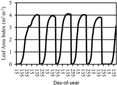
The bracket in the horizontal axis represents the harvest window, and the middle of the bracket represents expected harvest date.
Figure 2 – Example of Leaf Area Index (LAI) development (simulated) for a typical sugarcane crop cycle (one plant cycle and four ratoon cycles) in southeast Brazil.
For all crops, planting date may be either prescribed or determined by the model. The model’s decision to plant a crop is based on three conditions: The 10%day running averages of both daily mean air temperature and minimum temperature must be higher than specified thresholds. Furthermore, planting cannot take place before a specific date based on the typical growing season across the region in question. All three conditions must be met for planting to take place.
For annual crops, harvest takes place when both GDD (Growing Degree Days, thermal time in units of oC per day accumulated since planting) is equal or higher than GDDm (GDD to achieve physiological maturity) and the day during the integration is higher than the specified day%of%year set as the earliest harvest day. For sugarcane, the harvest takes place in a specified harvest window between a minimum and maximum day%of%year (represented in Figure 2 by a bracket). Then, as in the other crops, sugarcane is harvested (in the harvest window) when GDD reaches GDDm. In the literature, a base temperature between 8oC and 15oC is used to compute the GDD for sugarcane (KEATING et al., 1999) and Agro%IBIS uses a base temperature of 12oC. Since
0 1 2 3 4 5
15 135 255 15 135 255 15 135 255 15 135 255 15 135 255 15 135 255 15 135
L
ea
f
A
re
a
Inde
x
(
m
2m 2)
the model is designed to run from site to global scale, the thermal time to reach physiological maturity is not a pre%specified crop GDDm but is calculated interactively during integration based on the normal planted crop growth period, days between planting, and expected harvest date (date centered between maximum and minimum harvest days). A first approximation for GDDm is calculated based on annual climatology, for a given grid point, and then for every crop cycle this value is interactively updated based on temperature during integration. A maximum defined hybrid GDDm can also be specified. After the sugarcane is harvested the consecutive ratoons are grown until the same harvest window.
In addition to the plant and harvest controls, the crop management module also considers nitrogen fertilization and irrigation. Fertilization is applied every planting date, and the amount of N per hectare applied is pre%specified, either fixed for each crop type or varied according to an input file. However, due to the lack of information on level of fertilization, soil nitrogen content, impact of pre%harvest fire on nitrogen emission/deposition in the present simulations, the nitrogen impact on photosynthesis was not considered and nitrogen stress functions was considered as non%limiting. Irrigation, if applied, can be either specified or calculated during the integration based on average daily water content in the soil (the amount of water applied to a managed ecosystem was computed on a daily basis).
incorporated into litter (based on SOUZA et al., 2005), and the remaining is assumed to be burnt.
321262 . -/ ) " ')($ ) ')!
Agro%IBIS has different methodologies to account for the phenology and carbon (C) allocation of crop and natural ecosystems. For annual crops, Agro% IBIS considers three key growth stages controlled by GDD: (i) from planting to leaf emergence; (ii) from leaf emergence to end of silking; (iii) from grain fill to physiological maturity. Each phenological stage is characterized by different C allocation fractions to the four specific C pools (i.e., leaf, stem, root, and grain) based on CERES%Maize and EPIC models (KUCHARIK; BRYE, 2003). Leaf emergence occurs when the GDD is higher than a specific percentage of the GDDm. The second phase goes from leaf emergence to end of silking, at which time most of NPP goes to leaves and roots. The third phase, grain fill to senescence, is characterized by grain formation.
For the sugarcane crop, a new carbon allocation scheme was implemented. Based on an analysis of the two main international sugarcane crop models, APSIM%Sugarcane (KEATING et al., 1999) and CANEGRO (SINGELS; BEZUIDENHOUT, 2002; SINGELS et al., 2005) we developed a new Agro%IBIS carbon allocation scheme, drawing heavily on the CANEGRO model equations. Our first modification in the original CANEGRO C allocation set of equations was to consider the allocations as a function of GDD, instead of accumulated biomass (since it is not possible to know the typical crop biomass for all grid points). As mentioned above, in grain crops such as soybean and maize, daily NPP is allocated to the four carbon pools: leaves, roots, grains and stem. Analogously, in the sugarcane module daily NPP is allocated to four carbon pools: leaves (Al), roots (Ar), stem sucrose (Asuc), and structural stem
(Astc % stem fibre plus non%sucrose material). First, daily NPP is divided between
aerial (Aa % all above ground biomass), roots (Ar), and stem (Astm) C pools,
where Astm includes Asuc plus Astc:
1 1, 1 e (1)
"# $ % & % $ % (3)
1 e '()*(+ ,()*(+ '()*(+ ! (4)
"# 100 -.//.//+0 (5)
Where RM is the crop relative maturity, Rd is the root decline coefficient,
and Arm and Alm are the minimum fraction of carbon allocation to roots and
leaves, respectively. RM expresses the evolution in GDD along the crop cycle in a scale that ranges from 0 to 100. It normalizes the spatial variability of GDD and is computed for each grid point interactively. F1 and F2 are the linear and
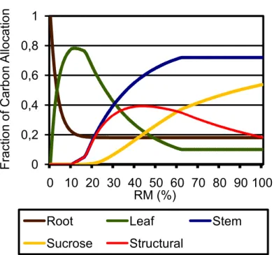
exponential functions that describe stem allocation; the maximum value of these two functions composes the allocations to stems (Astm) (Figure 3). These
functions are based on the principle that carbon allocation to stems is nearly linear in the beginning of sugarcane growth and then follows a logarithmic profile for the rest of crop cycle (see KEATING et al., 1999 for some observational evidence).
Figure 3 – Fractional carbon allocation to the different carbon compartments in sugarcane along crop cycle: root (brown line), leaves (green line), stalk (cane % blue line), structural (red line), and sucrose (yellow line).
0 0,2 0,4 0,6 0,8 1
0 10 20 30 40 50 60 70 80 90 100
F
ra
ct
io
n
o
f
C
a
rb
o
n
A
llo
ca
ti
o
n
RM (%)
Root Leaf Stem
F1 (Eq. 3) is a linear function of RM (Eq. 5), Clstem is the angular
coefficient of F1 and the product between Clstem times Ilstem determines the GDD
for which F1 is greater than 0.0. Therefore, Clstem and Ilstem define when carbon
starts to be allocated to structural stem (when F1 and F2 are lower than 0.0 they
are not accounted for Astm – there is no negative allocation). For example, a
Ilstem (linear intercept point) of 10 (Figure 3) signifies that the linear allocation to
Astm starts when RM is equal to 10 (or GDD is equal to 10% of GDDm).
F2 (Eq. 4) is an exponential function of RM (Eq. 5). The coefficient
Cestem determines the exponential function F2 and the product between Cestem
and Iestem establish the GDD for which F2 is greater than 0.0; therefore, Cestem
times Iestem defines when the exponential function F2 can potentially (i.e., F2
greater than F1 and zero) direct carbon allocation to the structural stem. For
example, Ilstem (exponential intercept point – RM for which F2 is equal to zero) is
equal to 15 in Fig. 3, meaning that F2 is greater than zero from RM higher than
15 (or GDD higher than 15% of GDDm).
In addition, root allocation (Ar) is the complement of Aa to the unit, and
leaves allocation (Al) is given by (Aa % Astm). Following the same form of
functions, carbon allocated to stem (Eq. 2) is then partitioned between stem sucrose (Asuc), and structural stem (Astc) following the set of equations:
12 % 0, 3, 4 (6)
3 "# $ 12 & 12 $ 12 (7)
4 1 e '()56 ,()56 '()56 ! (8)
Finally, the carbon content of each organ is updated on a daily basis by accumulating the daily NPP allocated to each organ fraction and subtracting the organ turnover (considered to occur only for leaves and roots). Although leaf turnover in sugarcane depends on temperature, leaf age, light competition, and water stress (e.g., KEATING et al., 1999; SMITH; SINGELS, 2006), leaf and root turnover are simulated as the product between the carbon content in each pool and a constant turnover rate. Additionally, leaves are considered to decay if temperature drops below water freezing point. The physical proprieties of the canopy (e.g., reflectance, transmittance, canopy water storage and heat capacity) are modeled as a function of the carbon accumulated to leaves and stem, and LAI is given by the product of carbon in the leaf pool and a constant specific leaf area (SLA % m2.kg%1).
3232 ) ")! ) " ,#! ")!) !
Four different datasets of increasing spatial scale were used to validate the yield simulated by the sugarcane module: (i) micro%meteorological and biomass observations, obtained for one crop cycle (391 days) in northern São Paulo state (Brazil), (ii) yield from two consecutive ratoons grown with three different irrigation regimes at an experimental site at Kalamia estate, Australia; (iii) sixteen years of yield data for the four largest sugarcane producing meso% regions in the Brazilian state of São Paulo; (iv) annual average yield over 31 years for the U.S. state of Louisiana.
323212 7 )# !)! 8, ( !) !
observations for the preceding cycle, the days between 38 and 104 of 2005 are only shown as reference points for the analyzed crop cycle and were not considered in the analyses.
The granulometric analysis showed a mean (first 2 m) soil composition of 22% of clay, 3% of silt and 74% of sand. The regional climate is typically warm and wet in the summer, and mild and dry in the winter (see TATSCH et al., 2009). Both temperature and precipitation show a marked annual cycle. The mean monthly temperature varies between 19oC in June and 24oC in February, with a mean annual temperature of 22oC. The mean monthly rainfall is about 50 mm in the dry season and reaches more than 200 mm during wet season.
The model was forced with meteorological data from an automatic weather station. The data were sampled every 10s and registered as 10 min averages in a datalogger (CR10X, Campbell Systems). Hourly average means of air temperatures, global solar radiation, relative humidity, surface pressure, wind speed, and daily precipitation were used as input for the simulation. Tatsch et al. (2009) provide a detailed description of the experimental site, meteorological and biomass datasets. Micro%meteorological measurements made over sugarcane at the São Paulo state are also described in Cabral et al. (2003) and Rocha et al. (2000). Validations include sensible heat flux (H), latent heat flux (λE) and carbon dioxide flux (which is compared against modeled net ecosystem exchange NEE) derived from the eddy covariance technique. In all simulations, model was integrated considering 11 soil layers, with a total soil depth of 2.5 m.
323232 9) ) ) !)! 8, ( !) !
used at an estimated rate of 1.00xET0 (1.00ET0) and 1.25xET0 (1.25ET0), where ET0 is the reference evapotranspiration (ALLEN et al., 1998). The third treatment was conventional furrow irrigated (FRW), providing at least 70 mm of water when a soil available water deficit of about 70 mm had developed. This deficit was calculated using the estimated evapotranspiration rate of 1.25xET0.
The experimental site was divided into 12 plots, 4 replications for each treatment. Each plot consisted of nine rows 1.52 m apart and 39 m long. All plant and soil measurements were taken from the four inner irrigated rows (net plot). Complete information about the field experiment is given by Inman% Bamber and Attard (2008). Simulations were forced with daily meteorological observations made at the site, and daily irrigation (see Figure 4, gray columns) follows the daily field observations for each treatment.
323262 7 )# (
and anomalies also consider one year average, from August to August; anomalies were derived from the 1990%2005 mean.
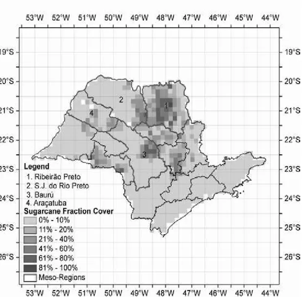
The four mesoregions considered in the simulations are indicated by the numbers: (1) Ribeirão Preto; (2) São José do Rio Preto; (3) Bauru; (4) Araçatuba. Grid corresponds to the terrestrial grid used by Agro%IBIS (0.5o), which is the same as the CRU monthly climate dataset. Percentage under sugarcane cultivation (fractional cover) for each pixel (~0.16o) is plotted over the map (shaded field), based on the IBGE's 1995 census.
3232:2 # ) ) !)!
The third validation compares simulated results over a 0.5º x 0.5º grid against statewide yield for the U.S. state of Louisiana. Estimated yields were taken from Greenland et al. (2005). The dataset was produced by the American Sugarcane League and the period used for validation goes from 1963 to 1993. The model was integrated from 1958 to 1993 for all Louisiana State grid points and state yield average considers the grid points following the main sugarcane cultivated area presented by Greenland et al. (2005).
62
6212 7 )# !)! 8, ( !) !
621212 ) $ ) ) " ()" )! % #8
Hourly radiation intercepted by canopy is given by the nature of incident radiation (direct or diffuse), incidence angle, leaves and stem area index, radiation extinction coefficient, and leaves and stem reflectances at each waveband. The process adopted to adjust reflectances followed three interactive steps: (i) adjustment of carbon allocation to leaves pool (i.e., LAI); (ii) adjustment of radiation extinction coefficient, and; (iii) adjustment of green and brown (dead) leaves reflectances.
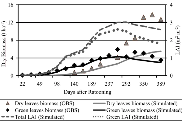
dependent on cultivar and environmental conditions, and the 5.7 m2⋅kg%1 observed is relatively low compared with typical range of published values (e.g., PELLEGRINO, 2001; PINTO et al., 2006). Assuming the observed total green leaves maximum (average) of 5.5 t⋅ha%1 (Figure 5 – dry matter) results in an observed maximum LAI of around 3.1 m2⋅m%2 (0.55 kg⋅m%2 times 5.7 m2⋅kg%1), while the maximum simulated green LAI was 2.7 m2⋅m%2 (Figure 5).
Figure 5 – Observed (symbols) and simulated (lines) dry matter accumulation in green (black) and dead (dark gray) leaves during the ratoon cycle. Simulated total (green plus attached dead, dark gray dashed line) and green (light gray dotted line) LAI are displayed in the right axis.
0 1 2 3 4
0 4 8 12 16
22 49 98 140 189 237 292 350 389
L
A
I
(m
2 m 2 )
D
ry
B
iom
as
s
(t
ha
1 )
Days after Ratooning
Dry leaves biomass (OBS) Dry leaves biomass (Simulated)
Green leaves biomass (OBS) Green leaves biomass (Simulated)
Agro%IBIS simulates leaf decay as the product between foliage biomass and a constant turnover time. Even using a relative low (related to the others cultures) value for average leaf resident time (175 days) simulated dead leaves dry biomass is underestimated. Although the simulated value is much lower than observed, the observed and simulated dead leaves values are in the range of values reported in literature (e.g., THOMPSON, 1978; ROBETENSON et al., 1996; INMAN%BAMBER et al., 2002).
Two different procedures were adopted to calibrate the radiation extinction coefficient, both based on the assumption that LAI and SAI (stem area index) had been accurately simulated. Radiation extinction coefficient (Ke) in IBIS depends on three parameters (leaf orientation, transmittance and reflectance) and two diagnostic variables (LAI and SAI). Leaf orientation along with LAI determines the leaf projected area in the beam direction. Typically, leaf angle departure (χL) is assumed to be %0.5 for C4 species (χL ranges from %1 for vertical leaves, 0 for randomly oriented, 1 for horizontal leaves).
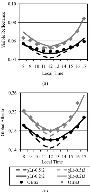
The sensitivity of the simulated reflectance was assessed for phase 2 and phase 3 using two different values for χL (%0.5 and %0.2) (Figure 6). Phase 2 is the full canopy phase (from day 270 of 2005 to 48 of 2006) and is characterized by low albedos. Phase 3 is the senescence period (from day 68 to 130 of 2006) during which green/brown LAI gradually reduces/increases, and albedos increase. The best fit to the observed values was achieved when χL was set at %0.2.
Simulated total solar radiation flux (Rs) attenuation by canopy resulted
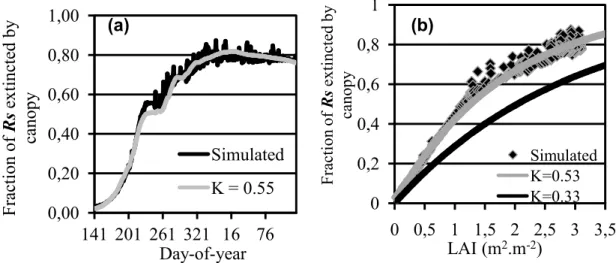
in an estimated Ke (radiation extinction coefficient) of 0.55 (Figure 7a). Although 0.55 is relative high in the range of sugarcane observations (0.37%0.53) reported by Park et al. (2005), it is consistent with their observation that tropical locations are characterized by high Ke. It is also important to note that Ke differs between crop classes, cultivars, and soil and climatic conditions (ROBERTSON et al., 1996; PARK et al., 2005). The relationship between intercepted Rs and LAI
(a)
(b)
Figure 6 – Observed (symbols) and simulated (solid and dashed lines): (a) visible reflectance and (b) global solar albedo diurnal cycle averaged for two periods, full canopy (black) and senescence (gray) period. Simulations differ in the leaf angle departure (χL); see text for details.
0,04 0,06 0,08 0,10
8 9 10 11 12 13 14 15 16 17
V
is
ibl
e
R
ef
le
ct
anc
e
Local Time
0,14 0,18 0,22 0,26
8 9 10 11 12 13 14 15 16 17
G
loba
l
A
lbe
do
Local Time
χL( 0.5)2 χL( 0.5)3
χL( 0.2)2 χL( 0.2)3
Figure 7 – Fraction of total solar radiation flux (Rs) extincted by canopy
integrated by model (black line) along the crop cycle and analytical solution of analogous Beer%Lambert law (gray line) with extinction coefficient (Ke) of 0.55 (best fit to the simulated Rs
extinction) (a); Rs extincted by canopy as function of LAI
integrated by model (black symbol) and according to Beer% Lambert law using Ke = 0.33 (black line) and 0.53 (gray line); values of Ke reported by Park et al. (2005) (b).
The model produced a very close concordance between daily simulated and observed surface Rs and photosynthetic active radiation flux (Rp)
reflectances (Figure 8) – solar radiation is separated in two wavelength bands (visible from 0.4 to 0.7 bm and near%infrared from 0.7 to 4.0 bm). In the day after harvest (day 108 of 2005) Rp reflectance leaps from 0.05 to 0.1 in both
observation and simulation. Aerial biomass not harvested (top and leaves) was left over ground and burned around day 140, as seen by the drop in observed albedo (Rs reflectance). Although the model successfully simulates the increase
in albedo after harvest, in the days between harvest and biomass burn the simulation somewhat deviates from observations (Rp reflectance). This is
attributable to the fact that Agro%IBIS does not have a module to account explicitly the management of aerial biomass not harvested – leaves were considered to be burnt on the harvest day and any remaining meristem was incorporated into the litter pool. Field observations indicate that both reflectances remain high until the day the fields are burnt, probably because of
0,00 0,20 0,40 0,60 0,80 1,00
141 201 261 321 16 76
F ra ct ion of R s ex ti nc te d by ca nopy
Day of year Simulated
K = 0.55
0 0,2 0,4 0,6 0,8 1
0 0,5 1 1,5 2 2,5 3 3,5
F ra ct ion of R s ext inc te d by ca nopy
LAI (m2.m2)
Simulated K=0.53 K=0.33
straw left over ground, in contrast to simulated albedo that was derived from bare soil. After this initial stage, the simulation and observations show a similar pattern, indicating that Rs/Rp reflectances gradually increase/decrease as LAI
develops. As LAI grows, simulated Rp reflectance increasingly approaches
observations until it stabilizes at 0.05, when simulated LAI is around 2.0.
Figure 8 – Daily surface total solar radiation flux (Rs % dark gray) and
photosynthetically active radiation flux (Rp % black) reflectances,
observed (symbols) and simulated (solid lines) – right vertical axis scale. Total, green plus attached dead leaves, LAI (m2 m%2 – black dotted line) simulated is plotted in the left axis scale. Period goes from day 38 of 2005 to 129 of 2006.
0 0,05 0,1 0,15 0,2 0,25
0 1 2 3 4 5
38 83 128 173 218 263 308 353 33 79 124
R
ef
le
ct
anc
e
L
A
I
(m
2m 2)
Day of year
LAI (Simulated) Rp reflectance (Simulated)
621232 )($ $) ) ' ) " ), !() , ()!
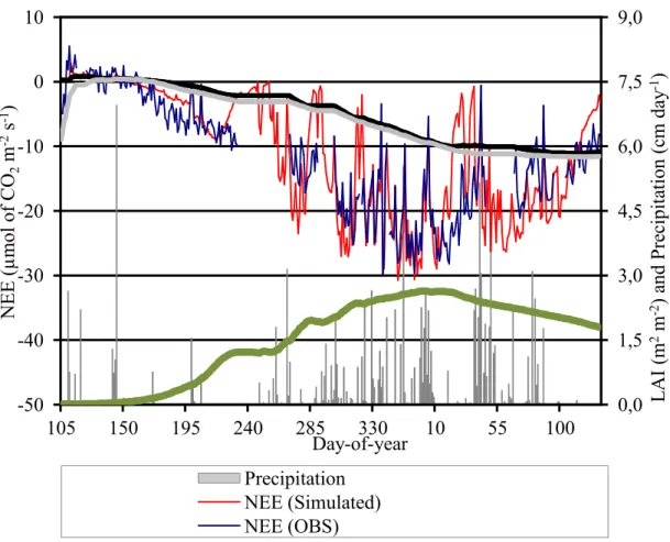
The seasonal photosynthetic cycle is robustly simulated by the model, although daily variability is best simulated for the period of maximum assimilation (Figure 9). Another clearly observable pattern is that simulated NEE drops sooner and to a greater degree than observed values during periods with low precipitation (e.g. between days 10 and 40 of 2006). The underestimation in this period is the major contributor to the final diurnal average NEE bias (%6.44%, as inferred from the deviations of the cumulative curves – Figure 9).
Figure 9 – Average diurnal (from 8 am to 18 pm, local time) CO2 net ecosystem exchange (NEE % bmol of CO2 m%2 s%1) observed (blue line) and simulated (red line). Cumulative NEE observed (gray line) and simulated (black line) are also plotted in the left axis. Green LAI (m2 m%2 – green dotted line) and observed precipitation (cm day%1 % background gray column) are plotted in the right axis scale. Period goes from day 105 (ratooning) of 2005 to 129 of 2006 (harvest).
0,0 1,5 3,0 4,5 6,0 7,5 9,0 50 40 30 20 10 0 10
105 150 195 240 285 330 10 55 100
L
A
I
(m
2m 2) a
nd P re ci pi ta ti on ( cm da y 1) N E E ( < m ol of C O2 m 2s 1)
Day of year
Diurnal cycles of NEE (Figure 10) were divided in three periods: (1) initial growth (from day 124 to 233 of 2005); (2) crop growth maximum (from day 270 of 2005 to 48 of 2006), and; (3) crop growth decline (from day 68 to 130 of 2006). The gaps between periods being caused by a lack observations during these times (illustrated in Figure 9). In the initial period Agro%IBIS underestimated NEE (Figure 10), this being most apparent after midday. In the second period of the cycle, assimilation increases with Rp flux until 11.00 am
and then gradually decreases after that (Figure 10). Although simulated and observed NEE show a high degree of concordance, modeled NEE tends to decreases relative to the observed data from 11.00 am to 4.00 pm. During the latter period the modeled results follow the observations closely throughout the entire diurnal cycle.
Figure 10 – Observed (symbols) and simulated (lines) average CO2 net ecosystem exchange (NEE % bmol of CO2 m%2 s%1) diurnal cycle for three periods: (1) initial growth (blue line and symbol); (2) maximum crop growth rate (red line and symbol); and (3) decline crop growth rate (black line and symbol).
30 25 20 15 10 5 0 5
8 9 10 11 12 13 14 15 16 17 18
N
E
E
(
<
m
ol
of
C
O2
m
2 s 1 )
Local Time
OBS (1) Simulated (1)
OBS (2) Simulated (2)
Simulated hourly NEE shows a similar relationship with air temperature to observed NEE (Figure 11a). NEE grows exponentially with temperature until a maximum assimilation around 27oC, and then drops shutting down for temperatures higher than 35oC. It is important to note that other factors also affect this relationship. For example, relative humidity (h) also has a strong influence over NEE, and h tended to vary from 20% to 40% for temperatures of about 35oC. The model also accurately simulates the relationship between photosynthesis and h (Figure 11b). When simulated NEE is plotted against observed NEE (Figure 11c), the general fit of the model is good (R2 = 0.69, relative bias %6.6%).
The model gives a generally robust simulation of ET (Figures 12a and 12b) as demonstrated by a strong correlation with observed values (R2 = 0.87), although there is a tendency of overestimation (0.32 mm day%1 on average) – with the exception of periods of soil exposure when LAI is below 1.0 m2 m%2. ET bias tends to be especially high in days following precipitation events, and tends to drop during dry periods. This pattern is driven by the soil water stress function, which tends to reduce photosynthesis and ET as soil dries.
(a) (b)
(c)
Figure 11 – Dispersion diagram between hourly net CO2 ecosystem exchange (NEE % bmol of CO2 m%2 s%1) and air temperature (above canopy – reference level), observed (gray symbol) and simulated (black symbol) (a); same as (a) for NEE and relative humidity (%) (b); dispersion diagram between hourly observed and simulated NEE (c). 60 50 40 30 20 10 0 10
5 10 15 20 25 30 35 40
N E E ( < m ol of C O2 m 2s 1)
Air Temperature (oC)
Simulated OBS 60 50 40 30 20 10 0 10
20 30 40 50 60 70 80 90 100
N E E ( < m o l o f C O2 m 2s 1)
Relative Humidity (%)
Simulated OBS
(a)
(b)
Figure 12 – Daily ET (evapotranspiration – mm day%1) observed (gray line) and simulated (black line) (a); dispersion diagram between observed and simulated daily ET (mm day%1) (b).
0 1 2 3 4 5 6
38 83 128 173 218 263 308 353 33 79 124
E
T
(
m
m
d
a
y
%1)
Day%of%year Simulated OBS
0 1 2 3 4 5 6
0 1 2 3 4 5 6
S
im
ul
at
ed
E
T
(
m
m
da
y
1)
(a) (b)
(c)
Figure 13 – Dispersion diagram between hourly ET (evapotranspiration – mm hour%1) and air temperature (above canopy – reference level), observed (gray symbol) and simulated (black symbol) (a); same as (a) for ET and relative humidity (%) (b); dispersion diagram between hourly observed and simulated ET (c).
0,0 0,1 0,2 0,3 0,4 0,5 0,6 0,7 0,8
5 10 15 20 25 30 35 40
E T ( m m h o u r 1)
Air Temperature (oC)
Simulated OBS 0,0 0,1 0,2 0,3 0,4 0,5 0,6 0,7 0,8
10 20 30 40 50 60 70 80 90 100
E T ( m m h o u r 1)
Relative Humidity(%)
Simulated OBS 0,0 0,2 0,4 0,6 0,8
0 0,2 0,4 0,6 0,8
S im ul at ed E T ( m m hour 1)
ET underestimation resembles NEE and air temperature relationship (Figure 14a), suggesting that this relationship is (as expected) related with stomatal opening. Maximum ET bias occurs at temperatures around 30oC, indicating a concomitant effect of temperature via water vapor pressure deficit. However, there is no clear relationship between ET bias and h (R2 = 0.003; Figure 14b), with the maximum observed bias for h between 40 and 70% (coincident with temperatures of around 30oC).
Figure 14 – Dispersion diagram between ET (evapotranspiration – mm hour%1) bias against: (a) air temperature (oC) and (b) relative humidity (%).
The modeled relationship between NEE and absorbed solar radiation is generally similar to observations (Figure 15). NEE over absorbed solar radiation (ARs) increases almost linearly until a maximum is reached around day 340 of
2005 (some days before green leaf biomass reaches its maximum – Figure 5, DAR 237), and model overestimates this increase after day 249. Although result is close to the observations during the maximum photosynthetic active period, the model tends to be over sensitive to dry events. During the final phase of crop cycle, the model tends to overestimate the rate of NEE/ARs – with
exception of final days of the cycle when the model responds more intensely to water shortage. Most of literature reports radiation use efficiency (RUE) as the
R² = 0,135 0,4
0,0 0,4 0,8
0 10 20 30 40
E T bi as ( m m hour 1)
Air Temperature (oC)
R² = 0,003 0,4
0,0 0,4 0,8
20 40 60 80 100
E T bi as ( m m hour 1)
Relative Humidity (%)
rate of aerial dry biomass per MJ of solar radiation intercepted (e.g., 1.59 g MJ%1 for ratoon crop; ROBERTSON et al., 1996). This cannot be derived from observations in the current study as solar radiation just below green canopy was not measured. Modeled NPP over%absorbed solar radiation by total green leaves was 1.9 g MJ%1 during the full canopy period, which is consistent with potential (non stressed) 2.12 g MJ%1 value reported by Singels and Bezuidenhout (2002) and field values reported by Muchow et al. (1999).
Figure 15 – Observed (gray line) and simulated (black line) daily rate between CO2 net ecosystem exchange (NEE % in dry matter base) and surface absorbed solar radiation (ARs – MJ m%2 day%1). Simulated
LAI (m2 m%2 – black dotted line) is plotted in the right axis scale.
The ratio between simulated NEE and ET, a measure of water use efficiency, follows observations closely across the entire crop cycle (Figures 16a and 16b). NEE/ET starts to drop around day 147 then decreases faster until day%of%year 210. This decline continues until about day%of%year 336, which
0 1 2 3 2 1,5 1 0,5 0 0,5 1
105 150 195 240 285 330 10 55 100
L A I (m 2m 2) D ai ly N E E / A Rs (g of dr y m at te r pe r M J)
Day of year
NEE/ARs (Simulated) NEE/ARs (OBS)
coincides with maximum green leaves biomass. Observed and simulated dispersion between NEE and ET present similar linear regressions (Figure 16b).
(a)
(b)
Figure 16 – Observed (gray line) and simulated (black line) daily CO2 net ecosystem exchange (NEE % gCO2 m%2 day%1) over evapotranspiration (ET – kg m%2 day%1). Simulated LAI (black dotted line % m2 m%2) is plotted on the right axis scale (a); dispersion diagram between daily NEE (gCO2 m%2 day%1) and ET (kg m%2 day%1) (b).
0 1 2 3 4 20 10 0 10 20
105 150 195 240 285 330 10 55 100
L A I (m 2m 2) D ai ly N E E /E T ( g o f C O2 p er K g o f H2 O )
Day of year
NEE/ET (Simulated) NEE/ET (OBS) LAI (Simulated)
R² = 0,743
R² = 0,721
60,0 40,0 20,0 0,0 20,0
0,0 2,0 4,0 6,0
N E E ( g C O2 m 2d ay 1)
ET (Kg H2O m2day1) NEE
Dry biomass observations made in the micro%meteorological experiment go from June 5th of 2005 (22 days after ratooning % DAR) to May 10th of 2006, two days before harvest (389 DAR). Total green leaves dry biomass is accurately simulated, with a slight underestimation from the middle until the end of cycle (Figure 17). Total dead leaves dry biomass is overestimated at the beginning of cycle and underestimated from 140 DAR onwards. Cane biomass is robustly simulated for most points along the crop cycle. The main deviations occurred from day 327 to 375, with final biomass converging again with observations (final relative bias equal to %6.23%). Total aerial biomass is underestimated from 140 DAR onwards. Most of the underestimation is related to total dead leaves biomass, which was relatively high compared to other published locations (e.g., ROBETENSON et al. 1996; INMAN%BAMBER et al., 2002).
Figure 17 – Observed (symbols) and simulated (lines) dry biomass (t ha%1) accumulated along the ratoon cycle: total aerial (black), cane (blue); dead (dry) leaves (brown), and green leaves (green). 0
10 20 30 40 50 60
22 49 98 140 189 237 292 350 389
D
ry
B
io
m
a
ss
(t
h
a
%1 )
Days After Ratooning Total (Simulated)
621262 (-/ $) ) '
Net radiation (Rn) is underestimated by the model when soil is exposed
(Figure 18). As the canopy grows simulated Rn converges with observations,
and bias tends to be less than 5.0%. Even though the simulation follows the observed decrease in the rate between Rn and ARs when soil is more exposed
(consistent with the high soil heat accumulation during the day and increase of thermal radiation lost during night, and less transpiration), Agro%IBIS overestimated the long wave radiation lost in the initial crop growth stage. Considering the entire cycle, the model shows a relative bias of %6.5% (R2 = 0.97).
Figure 18 – Observed (black) and simulated (gray) daily net radiation (Rn). Light
gray columns shows net radiation relative bias (%, scale in the right axis).
60 0 60 120
10 0 10 20
38 128 218 308 33 123
Rn
B
IA
S
(
%
)
Rn
(M
J
m
2 da
y
1 )
Day of year
Daily soil temperature is accurately simulated by model (Figure 19). However simulated soil heat flux diurnal cycle shows a more pronounced amplitude (21d), highlighting the importance of considering a specific layer of dead biomass over the soil – thereby connecting the litter fall biomass with the energy and water balance. Despite a large amplitude in the diurnal cycle, the seasonal and diurnal variability of soil temperature is consistently simulated. The soil temperature overestimation during the period when vegetation cover is non%existent (Figure 19) was also reported by Kucharik and Twine (2007).
Figure 19 – Observed (at 2 cm, gray line) and simulated (first soil layer – 2.5 cm, black line) soil surface temperature (oC).
After harvest, the Bowen ratio (β) rises rapidly from around 0.5 to 2.0 (Figure 20). During this period β is strongly coupled to precipitation and is observed to drop after rain events and to increase as soil dries. As the canopy develops, β tends to decrease linearly until it reaches an average minimum of about 0.5 (observed) and 0.35 (simulated). Although the simulated energy partition seasonal cycle is consistently simulated, β is overestimated for low LAI
10 15 20 25 30 35
38 83 128 173 218 263 308 353 33 79 124
S
o
il
T
e
m
p
e
ra
tu
re
(
oC
)
Day%of%year
and underestimated for high LAI. The dispersion diagram of observed and simulated H and λE (Fig. 20b) shows that the model systematically under/overestimates H/λE with a relative bias of %10.5% (H) and 14.8% (λE) and an R2 equal to 0.68 (H) and 0.87 (λE).
(a)
(b)
Figure 20 – Observed (black line) and simulated (gray line) daily Bowen ratio (β % Sensible over Latent heat fluxes). Simulated LAI (m2 m%2, dotted black line) is shown as references (a); dispersion diagram between daily observed and simulated Sensible (H % black symbol) and Latent (λE % gray symbol) heat fluxes (MJ m%2 day%1) – linear regressions and R2 are shown for each dispersions (b).
0 0,5 1 1,5 2 2,5 3
38 83 128 173 218 263 308 353 33 79 124
B o w en r at io a n d L A I (m 2m 2)
Day of year
LAI (IBIS) b (Simulated)
b (OBS) 3 0 3 6 9 12 15
3 0 3 6 9 12 15
S im u la te d H an d λ E (M J m 2 d ay 1)
The diurnal cycle of energy balance components (Figure 21) was separated in two periods: (i) canopy development (from day 124 to 233 of 2005), (ii) full canopy cover (from day 270 of 2005 to the end of crop cycle). Average Rn is accurately simulated in both periods, showing only small
deviations in the first phase when the soil is exposed.
In the first crop period, the model simulates too much heat being conducted into the soil during the morning and, consequently, soil heat flux (G) is overestimated (Figure 21d) and H (Figure 21c) is underestimated. Only after 12.00am do G and H converge with observations. Excess heat accumulated in the soil is conducted back to the surface around sunset, and most of it is lost as long wave radiation after sunset (Figure 21a). λE is underestimated during the entire diurnal period (Figure 21c).
Figure 21 – Observed (symbols) and simulated (lines) diurnal cycle energy balance components averaged for two periods: (1 – gray) during canopy development; (2 % black) for full canopy cover. (a) Net radiation (Rn – W m%2), (b) Latent heat flux (λE – W m%2), (c)
Sensible heat flux (H – W m%2), and (d) Soil heat Flux (G – W m%2).
;)< ;$<
6232 9) ) ) !)! 8, ( !) !
The final simulated LAI was very similar to observed for the three experiments (Figure 22), although simulated LAI deviated from the observed value at 199 DAR (days after ratooning) for the 1.00ET0 and FRW treatments. In the second ratoon cycle there were no LAI observations. Here, the LAI simulations showed a greater difference between 1.25ET0 and FRW than in the first cycle, in part because initial LAI development occurred in a relative drier period in the second ratoon (see black bars in Figure 23a%c).
Figure 22 – Observed (symbols) and simulated (lines) LAI (m2 m%2) over two consecutive ratoon cycles for the three irrigation treatments: 1.00 x ET0 (black), 1.25 x ET0 (dark gray), and furrow irrigation (light gray).
The model slightly underestimated ET at the beginning of ratoon cycles, but closely followed estimated values (gray symbols) in the middle of the cycle (Figure 23a%c). In the first ratoon cycle, ET increased quickly during the first months due to high solar radiation flux and rapid LAI development (The first ratoon starts in September and the second one in July). At the end of the first
0 1 2 3 4 5
1 61 121 181 241 4 64 124 184 244 304 364
L
A
I
(m
2 m 2 )
Days After Ratooning (DAR)
Simulated (FRW) OBS (FRW)
Simulated (1.25ETo) OBS (1.25ETo)
cycle the different irrigation regimes resulted in significant ET differences. The last irrigation application in the 1.00ET0, 1.25ET0, and FRW treatments were 33.9 mm (236 DAR), 43.8 mm (236 DAR), and 112.6 mm (241 DAR), respectively. In the days following these last irrigations, ET decreased exponentially in both 1.00ET0 and 1.25ET0, while ET decreased linearly in FRW (mainly following a reduction in radiation rather than soil moisture). Although the model slightly overestimated ET at the end of first ratoon cycle in 1.00ET0 and 1.25ET0, responses of ET to different irrigation regimes were robustly simulated. Observed and simulated datasets were characterized by higher ET during most of dry season in the second ratoon cycle (300 DAR). This increased ET during this period is probably associated with higher levels of irrigation.
The dispersion diagram between observed and simulated results indicated that the model tended to underestimate ET in all range of ET values and for all experiments (Figure 23d). Experiment 1.00ET0 had the lowest bias (relative bias were %10.1%, %12.5%, and %12.1% for the 1.00ET0, 1.25ET0 and FRW, respectively), and the experiment 1.25ET0 presented the lowest correlation coefficient (for the 1.00ET0, 1.25ET0 and FRW experiments were 0.83, 0.85, and 0.84, respectively).
(a) (b) 0 30 60 90 120 150 0 3 6 9 12 15
1 61 121 181 241 4 64 124 184 244 304 364
P re c. a nd I rr ig . (m m da y 1 ) E T ( m m da y 1)
Days After Ratooning (DAR)
Precipitation Irrigation Simulated OBS
0 30 60 90 120 150 0 3 6 9 12 15
1 61 121 181 241 4 64 124 184 244 304 364
P re c. a nd I rr ig . (m m da y 1) E T ( m m da y 1)
(c)
(d)
Figure 23 – Observed (gray symbol) and simulated (black line) daily evapotranspiration (ET – mm.day%1) for the three different irrigation treatments (see text): (a) 1.0xET0 irrigation; (b) 1.25xET0 irrigation; and (c) Furrow irrigation. Precipitation (dark column) and Irrigation (gray column) are plotted in the right axis. (d) Dispersion diagram between observed and simulated daily ET: 1.0xET0 irrigation (gray circles), 1.25xET0 irrigation (red diamonds), and furrow irrigation (black squares).
0 30 60 90 120 150 0 3 6 9 12 15
1 61 121 181 241 4 64 124 184 244 304 364
P re c. a nd I rr ig . (m m da y 1 ) E T ( m m da y 1)
Days After Ratooning (DAR)
0 2 4 6 8 10
0 2 4 6 8 10
S im ul at ed E T ( m m da y 1 )
Observed ET (mm day1)
FRW
1.25ETo
Figure 24 – Observed (symbols) and simulated (lines) above ground dry biomass (kg m%2) over two consecutive ratoon cycles for the three irrigation treatments: 1.00 x ET0 (black); 1.25 x ET0 (dark gray); and furrow irrigation (light gray).
6262 7 )# (
-Simulated average yield for the four São Paulo state mesoregions (Figure 25) were generally in good agreement with observed data, with a relative bias of less than 1.1%. Ribeirão Preto had the highest observed yield (79.4 t.ha%1), followed by Bauru (77.9 t.ha%1), São Jose do Rio Preto (76.9 t.ha%1), and Araçatuba (75.9 t.ha%1). The model accurately captured this spatial variability, simulating the highest yield for Ribeirão Preto (80.4 t.ha%1), followed by Bauru (77.4 t.ha%1), São Jose do Rio Preto (76.4 t.ha%1) and Araçatuba (76.4 t.ha%1).
0 2 4 6 8
1 61 121 181 241 4 64 124 184 244 304 364
A
bove
G
round D
ry
B
iom
as
s (
kg
m
2)
Days After Ratooning (DAR)
Simulated (FRW) OBS (FRW)
Simulated (1.25ETo) OBS (1.25ETo)
Figure 25 – Average (1990%2005) observed and modeled sugarcane yield (t⋅ha%1) for the four mesoregions.
The pattern of dispersion between observed and simulated yield for all points (sixteen years and four mesoregions, Figure 26a) suggested that Agro% IBIS did not have any major systematic biases, and the points oscillated around the 1:1 line (RMSE = 3.6 t ha%1). There were two outliers corresponding to yield underestimations in 2000 (Figures 27a and 27d), see in Figure 26c that model tended to overestimate the yield correlation with precipitation. Relative bias for all points was %0.15% with a correlation coefficient of 0.44.
The observed and modeled relationships between yield and growing season temperature (Figure 26b) were quite similar (giving almost identical quadratic regressions). Both regressions suggested a maximum yield for growing season temperature of around 23oC. Yield is positively correlated with precipitation (Figure 26c), and the model overestimated the strength of this relationship. The observed linear regression suggests that yield increased 2.19 t⋅ha%1 for each mm day%1, but the simulated response was 4.96 t⋅ha%1 for each mm day%1 (note that the range of precipitation variability varies from 2.5 to 5.0 mm day%1, or 912 to 1825 mm year%1).
75 76 77 78 79 80 81
Araçatuba Bauru Ribeirão
Preto
S. J. do Rio Preto
Y
ie
ld
(t
ha
1)
Meso Regions
(a)
(b) (c)
Figure 26 – Dispersion diagram between observed and simulated sugarcane yield for all years and mesoregions (black line shows the 1:1 relation) (a); observed (gray symbols) and modeled (black symbols) sugarcane yield (t ha%1), considering all years and mesoregions, against growing season (b) temperature (oC) and (c) precipitation (mm day%1). In (b) and (c) lines display the linear regressions. 65 70 75 80 85 90
65 70 75 80 85 90
S im ul at ed Y ie ld (t ha 1)
Observed Yield (t ha1)
São José do Rio Preto Ribeirão Preto Bauru Araçatuba 1:1 line 65 70 75 80 85
21 22 23 24 25
Y ie ld (t ha 1)
Temperature (oC)
Simulated OBS 65 70 75 80 85
2 3 4 5 6
Y ie ld (t ha 1)
Precipitation (mm day1)
Considering the results from all regions, the model showed a similar average and amplitude of yield fluctuations compared with the observed data (Figure 27a%d). In Araçatuba (Figure 27a) modeled yield was negatively correlated (r = %0.28) with observed yield, although by excluding the data for the year 2000 the correlation increased to 0.16 and model’s relative bias stayed low (from 0.73% to 1.7%). For the Bauru mesoregion (Figure 27b) simulated yield was similar to observed for most years (r = 0.41), and also produced a low relative bias (%0.56%). Interannual variability in yield for Ribeirão Preto (Figure 27c) follows the pattern observed in Bauru (Figure 27b), but with more pronounced oscillations. In Ribeirão Preto the model had a bias of 1.08% and correlation coefficient of 0.41. Finally, in São Jose do Rio Preto (Figure 27d), the observed and modeled data showed the highest interannual variability in yield. Relative bias was also low (%0.68%) and correlation with observed series was the highest (r = 0.50) among the simulations.
(a)
1 0 1 2 3 4 5
55 65 75 85
1990 1992 1994 1996 1998 2000 2002 2004 P
(
m
m
da
y
1)
and
T
(
oC
)
Y
ie
ld
(t
ha
1)
Temperature Precipitation
5
1 (b)
(c)
1 0 1 2 3 4 5
55 65 75 85
1990
1992
1994
1996
1998
2000
2002
2004
P (mm day1) and T (oC)
Yield (t ha1)
1 0 1 2 3 4 5
55 65 75 85
1990
1992
1994
1996
1998
2000
2002
2004
P (mm day1) and T (oC)