The influence of non-stationary ENSO teleconnections on reconstructions of paleoclimate using a pseudoproxy framework

(1)

CPD

11, 3853–3895, 2015

The influence of non-stationary teleconnections on

reconstructions of paleoclimate

R. Batehup et al.

Title Page

Abstract Introduction

Conclusions References

Tables Figures

◭ ◮

Back Close

Full Screen / Esc

Printer-friendly Version

Interactive Discussion

Discussion

P

a

per

|

Discussion

P

a

per

|

Discussion

P

a

per

|

Discussion

P

a

per

|

Clim. Past Discuss., 11, 3853–3895, 2015 www.clim-past-discuss.net/11/3853/2015/ doi:10.5194/cpd-11-3853-2015

This discussion paper is/has been under review for the journal Climate of the Past (CP). Please refer to the corresponding final paper in CP if available.

The influence of non-stationary ENSO

teleconnections on reconstructions of

paleoclimate using a pseudoproxy

framework

R. Batehup1,2, S. McGregor1,2, and A. J. E. Gallant3,2

1

Climate Change Research Centre, University of New South Wales, Sydney, New South Wales, Australia

2

ARC Centre of Excellence for Climate System Science (ARCCSS), Australian Research Council, Australia

3

School Earth, Atmosphere and Environment, Monash University, Victoria, Australia

Received: 15 July 2015 – Accepted: 25 July 2015 – Published: 24 August 2015

Correspondence to: S. McGregor (shayne.mcgregor@unsw.edu.au)

(2)

CPD

11, 3853–3895, 2015

R. Batehup et al.

Title Page

Tables Figures

◭ ◮

Back Close

Full Screen / Esc

Discussion

P

a

per

|

Discussion

P

a

per

|

Discussion

P

a

per

|

Discussion

P

a

per

|

Abstract

Reconstructions of the El Niño-Southern Oscillation (ENSO) ideally require high-quality, annually-resolved and long-running paleoclimate proxy records in the eastern tropical Pacific Ocean, located in ENSO’s centre-of-action. However, to date, the pa-leoclimate records that have been extracted in the region are short or temporally and

5

spatially sporadic, limiting the information that can be provided by these reconstruc-tions. Consequently, most ENSO reconstructions exploit the downstream influences of ENSO on remote locations, known as teleconnections, where longer records from pa-leoclimate proxies exist. However, using teleconnections to reconstruct ENSO relies on the assumption that the relationship between ENSO and the remote location is

station-10

ary in time. Increasing evidence from observations and climate models suggests that some teleconnections are, in fact, non-stationary, potentially threatening the validity of those paleoclimate reconstructions that exploit teleconnections.

This study examines the implications of non-stationary teleconnections on modern multi-proxy reconstructions of ENSO. The sensitivity of the reconstructions to

non-15

stationary teleconnections were tested using a suite of idealized pseudoproxy experi-ments that employed output from a fully coupled global climate model. Reconstructions of the variance in the Niño 3.4 index, representing ENSO variability, were generated us-ing four diﬀ_{erent methods to which surface temperature data from the GFDL CM2.1 was}

applied as a pseudoproxy. As well as sensitivity of the reconstruction to the method, the

20

experiments tested the sensitivity of the reconstruction to the number of non-stationary pseudoproxies and the location of these proxies.

ENSO reconstructions in the pseudoproxy experiments were not sensitive to non-stationary teleconnections when global, uniformly-spaced networks of a minimum of approximately 20 proxies were employed. Neglecting proxies from ENSO’s

center-of-25

(3)

CPD

11, 3853–3895, 2015

R. Batehup et al.

Title Page

Tables Figures

◭ ◮

Back Close

Full Screen / Esc

Discussion

P

a

per

|

Discussion

P

a

per

|

Discussion

P

a

per

|

Discussion

P

a

per

|

of pseudoproxies first, appeared to improve the robustness of the resulting tions. The results suggest that caution should be taken when developing reconstruc-tions using proxies from a single teleconnected region, or those that use less than 20 source proxies.

1 Introduction

5

Reconstructions of the Earth’s climate prior to instrumental records are necessary for providing context for anthropogenic climate change, and to provide insight into climate variability on time scales longer than instrumental records allow. Climate proxies are biotic or chemical analogues that have a sensitivity to some aspect of the climate, for example, oxygen isotope ratios in coral growth rings contain information on temperature

10

and precipitation (Pfeiﬀ_{er et al., 2004). Thus, these proxies are the essential tool for}

creating paleoclimate reconstructions. However, high quality proxies can be sparse and diﬃ_{cult to find (McGregor et al., 2010; Neukom and Gergis, 2012), limiting the}

amount of information that can be inferred about the climate.

One region where information from paleoclimate proxies is limited is the central and

15

eastern tropical Pacific Ocean. This area can be described as the centre-of-action of the El Niño-Southern Oscillation (ENSO), which is the most important regulator of inter-annual climate variability, globally. ENSO involves changes in eastern equatorial Pacific sea surface temperature (SST) and an associated swing in precipitation and pressure anomalies across the tropical Pacific Ocean. While its most noticeable eﬀ_{ects are in the}

20

tropical Pacific region, it also induces downstream eﬀ_{ects, influencing climate}

variabil-ity in many parts of the world via teleconnections (e.g. Power et al., 1998; Brönnimann et al., 2006; Liu et al., 2013; Ding et al., 2014).

Due to the global reach of ENSO, understanding its behaviour is of great societal and economic importance (Solow et al., 1998; McPhaden et al., 2006). There are still

un-25

(4)

Wit-CPD

11, 3853–3895, 2015

R. Batehup et al.

Title Page

Tables Figures

◭ ◮

Back Close

Full Screen / Esc

Discussion

P

a

per

|

Discussion

P

a

per

|

Discussion

P

a

per

|

Discussion

P

a

per

|

tenberg, 2010; Yeh et al., 2014). One reason for this is that the instrumental record is too short (∼150 years) to measure long term changes in ENSO and its teleconnections (Wittenberg, 2009; Gergis et al., 2006, references therein). Modelling suggests that five centuries of data may be required to understand the full range of natural ENSO vari-ability (Wittenberg, 2009). Thus, climate proxy reconstructions of past fluctuations in

5

ENSO are an essential tool in determining the full range of natural ENSO variability. As previously described, the centre-of-action of ENSO is largely devoid of long, con-tinuous, high-quality paleoclimate proxy records (Wilson et al., 2010). Tropical corals are the dominant proxy type in this region. However, their limited life span results in records that are on average about 50 yrs in length, with the longest records less than

10

two centuries (Cobb et al., 2013; Neukom and Gergis, 2012). This has motivated the use of paleoclimate proxies from single or multiple regions that are teleconnected with ENSO for the generation of reconstructions. For example, ENSO reconstructions have been developed using paleoclimate proxies from the south-west US and northern Mex-ico (D’Arrigo et al., 2005), northern New Zealand (Fowler, 2008) and using multiple

15

proxies from locations in the tropical and subtropical Pacific outside ENSO’s centre-of-action (Braganza et al., 2009; Wilson et al., 2010). Multi-proxy reconstructions are generally considered to be more robust and more likely to contain a larger climate signal to local noise ratio (Mann et al., 1998; Gergis and Fowler, 2009).

There are several issues when using teleconnected proxies for paleoclimate

recon-20

structions. Teleconnections may be non-linear in nature, for example, responding to El Niño events much more strongly than La Niña events (Hoerling et al., 1997). If this is not detected and accounted for in the reconstruction, ENSO variability and amplitude may be misrepresented (McGregor et al., 2013). However, perhaps an equally impor-tant issue, is the variability of the teleconnection itself. ENSO reconstructions exploiting

25

teleconnected locations implicitly assume that the teleconnected relationship does not vary significantly in time – that it is stationary. However, it is often diﬃ_{cult or}

(5)

CPD

11, 3853–3895, 2015

R. Batehup et al.

Title Page

Tables Figures

◭ ◮

Back Close

Full Screen / Esc

Discussion

P

a

per

|

Discussion

P

a

per

|

Discussion

P

a

per

|

Discussion

P

a

per

|

However, significant changes in the relationship between ENSO and the climates of remote, teleconnected locations have been detected in models (Coats et al., 2013; Gal-lant et al., 2013), instrumental observations (López-Parages and Rodríguez-Fonseca, 2012; Gallant et al., 2013) and paleoclimate data (Hendy et al., 2003; Rimbu et al., 2003; Timm, 2005). If these teleconnections were changed by some dynamical regime

5

rather than through stochastic influence (e.g. random weather events), the relation-ship should not be considered as stationary. While these dynamical changes could be related to external climate forcing, such as with anthropogenic climate change (Müller and Roeckner, 2008; Herceg Bulić_{et al., 2011), there is evidence that they also change}

with internal climate forcing. For example, significant changes in teleconnections on

10

near-centennial time scales are apparent in model simulations forced by internal dy-namics alone (Gallant et al., 2013).

The changes to teleconnections via internal dynamics will result from either changes to ENSO itself (i.e., changes in the spatial structure of the SST anomalies), or from non-linear interactions with other regulators of climate variability. An example of the

15

latter is the Southern Annular Mode, which is thought to aﬀ_{ect the magnitude of south}

Pacific ENSO teleconnections (Fogt et al., 2011). The evidence suggests that this oc-curs on time scales around 30 years or longer. Using running correlations as a sta-tistical descriptor of the relationship between ENSO and a remote climate variable, several studies highlighted that running correlations employing 11–25 year windows of

20

data exhibit large, stochastic variability only (Gershunov et al., 2001; Sterl et al., 2007; van Oldenborgh and Burgers, 2005). However, a study using longer windows of data spanning 31–71 years (Gallant et al., 2013), found that stochastic processes could not explain the changes in observed and modelled running correlations in a significant number of locations in Australasia. Similar results are also found using model

simula-25

(6)

ques-CPD

11, 3853–3895, 2015

R. Batehup et al.

Title Page

Tables Figures

◭ ◮

Back Close

Full Screen / Esc

Discussion

P

a

per

|

Discussion

P

a

per

|

Discussion

P

a

per

|

Discussion

P

a

per

|

tion as to whether non-stationarities have an appreciable influence on the robustness of past paleoclimate reconstructions.

This study examines if and when non-stationary teleconnections degrade the skill of multi-proxy reconstructions of ENSO variability by employing a series of pseudoproxy experiments from a fully coupled global climate model (GCM). The experiments test

5

how reconstruction skill varies with diﬀ_{erent proxy network locations and sizes. The}

sensitivity of the results to the reconstruction method is also tested. The model and the data used for these experiments is described in Sect. 2 and the methods are described in Sect. 3. The experimental outcomes are presented in Sect. 4, discussed in Sect. 5 and conclusions are provided in Sect. 6.

10

2 Model data

This study uses 500 years of a pre-industrial control run of the Geophysical Fluid Dy-namics Laboratory Coupled Model 2.1 (GFDL CM2.1) for all pseudoproxy experiments, which are described in detail in Sect. 3. ENSO is represented using the Niño 3.4 in-dex, calculated from the model as the area average of SST anomalies from the central

15

Pacific region (5◦S–5◦N, 190◦–240◦E). In the GFDL CM2.1 simulations, the monthly variations in the Niño 3.4 index very closely correspond to the variations of the first Empirical Orthogonal Function (EOF) of tropical Pacific SSTs, demonstrating that the Niño 3.4 index accurately represents ENSO variability in the model (Wittenberg et al., 2006).

20

Using climate data directly from GCMs is ideal for the evaluation of reconstruction methods (Zorita et al., 2003; Lee et al., 2008; von Storch et al., 2009) because models can provide the long time series necessary to robustly assess multidecadal to near-centennial scale variability in teleconnections (Wittenberg, 2009). The ENSO indices can be calculated directly from the model, representing a “true” Niño 3.4 index for the

25

(7)

CPD

11, 3853–3895, 2015

R. Batehup et al.

Title Page

Tables Figures

◭ ◮

Back Close

Full Screen / Esc

Discussion

P

a

per

|

Discussion

P

a

per

|

Discussion

P

a

per

|

Discussion

P

a

per

|

The GFDL CM2.1 simulation fixes all external climate forcings at 1860 levels. Thus, any changes to ENSO teleconnections will be the product of internal variability only. The model is fully coupled and comprises of the Ocean Model 3.1 (OM3.1), Atmo-spheric Model 2.1 (AM2.1), Land Model 2.1 (LM2.1), and the GFDL Sea Ice Simulator (SIS). The OM3.1 resolution is 1◦latitude by longitude with increasing resolution

equa-5

torward of 30◦, with 50 vertical layers and a tripolar grid (for more information see Griﬃ_{es et al., 2005). The AM2.1 and LM2.1 resolution is 2}◦ _{latitude by 2.5}◦ _longitude

with 24 vertical levels in AM2.1. For more information on AM2.1 and LM2.1, see Del-worth et al. (2006).

The GFDL CM2.1 was selected due to its realistic representation of ENSO

character-10

istics (Wittenberg, 2009, references therein). The seasonal SST structure and ENSO evolution is well represented when compared to observations (Wittenberg et al., 2006; Joseph and Nigam, 2006), while also matching their power spectra (Wittenberg et al., 2006; Lin, 2007). The representation of the strength of local teleconnections in the model, Fig. 1b, shows that the regional responses of surface temperature (TS) and

15

the Niño 3.4 index (shading) are quite similar to the observations (contours). Note that hereafter “TS” refers to SST temperatures over model ocean points and land surface temperatures over model land points. Hence, ENSO in the GFDL CM2.1 is imposing downstream eﬀ_{ects, i.e. teleconnections, that are broadly consistent with the}

observa-tions, even if the strength of the connection is not as is observed (Wang et al., 2012).

20

It has also been shown that the model teleconnections, represented by correlations in 31 year windows between grid points and the Niño 3.4 index generated from the model, do exhibit variability between periods and compared to correlations calculated over the entire period (Fig. 1a, Wittenberg, 2012). There is significant variation in teleconnection strength (i.e. the range of possible correlations) when using shorter windows of data

25

compared to those of the entire data set.

(8)

telecon-CPD

11, 3853–3895, 2015

R. Batehup et al.

Title Page

Tables Figures

◭ ◮

Back Close

Full Screen / Esc

Discussion

P

a

per

|

Discussion

P

a

per

|

Discussion

P

a

per

|

Discussion

P

a

per

|

nections that are poorly represented at the local level, particularly on the “edges” of the main teleconnections regions (e.g. on the coast of Australia and North America). This is due to inaccuracies in the representation of the mean climate, annual cycle, ENSO, and the other modes of climate variability that are influenced by, or which influence, ENSO, such as the Southern Annual Mode (Delworth et al., 2006). While this limits the

5

conclusions that can be drawn about real-world teleconnections, it still allows for an examination of reconstructions and the associated influence of the non-stationarity of teleconnections, internal to the GCM.

As ENSO events are generally synchronised to the seasonal cycle, the modelled TS was converted to June–July averages to capture ENSO event initiation and termination

10

within one year (Rasmusson and Carpenter, 1982; Tziperman et al., 1997). This has the added benefit of reducing 500 years of monthly TS data (6000 values) to 499 annual values, minimising the computational cost and matching the resolution of the majority of ENSO proxies. The 499 year mean was removed from the dataset and the grid point time series were then linearly detrended by calculating the residuals from a

line-of-15

best fit using linear regression, to remove long-term trends such as model drift. This modified TS dataset is used for all calculations and experiments in this study. Modelled precipitation, only briefly discussed in Sect. 4, was subjected to the same processing prior to any calculations.

3 Methods

20

(9)

CPD

11, 3853–3895, 2015

R. Batehup et al.

Title Page

Tables Figures

◭ ◮

Back Close

Full Screen / Esc

Discussion

P

a

per

|

Discussion

P

a

per

|

Discussion

P

a

per

|

Discussion

P

a

per

|

3.1 Pseudoproxy generation

The model TS and precipitation data were used to represent the climate proxies for all reconstructions. These data are commonly referred to as pseudoproxies and repre-sent a “perfect” proxy, free of non-climatic noise (von Storch et al., 2009). Unlike Lee et al. (2008), these pseudoproxies are not degraded by adding noise (which would add

5

realism), as the eﬀ_{ects of noise on the reconstructions are not in the scope of this}

study. Pseudoproxies are randomly selected from a subset of the globe, determined by several conditions, depending on the experiment. The most basic condition, present in all experiments, is that the absolute correlation between the model grid point and the Niño 3.4 index is above 0.3 in the calibration window. This threshold is an arbitrary

10

criterion that is simply there to ensure the pseudoproxies represent ENSO to some extent, making them at least partly relevant for reconstructing the ENSO signal. It is entrusted to the reconstruction methods to enhance the signal to noise ratio.

Networks of three to 70 pseudoproxies were used so that the eﬀ_{ect of increasing}

network size could be examined. The same pseudoproxy was not used in the same

15

network more than once, but could be used in multiple networks. One thousand random networks were selected and used to produce reconstructions of the model Niño 3.4 index. The randomised selection process over a large number of grid points means that there is only a very small chance that a network would be replicated within 1000 iterations.

20

The correlation at each grid point over the whole time period (499 years) and ENSO is assumed to represent the true teleconnection strength, as its use for calibrating the proxies should result in more accurate reconstructions. In reality, however, information is limited to the observational record. As such, calibration can only occur during a rela-tively brief period, which we expect to result in reconstructions that are not as accurate

25

as they potentially could be. To assess the eﬀ_{ects of the use of di}ﬀ_{erent calibration}

(10)

CPD

11, 3853–3895, 2015

R. Batehup et al.

Title Page

Tables Figures

◭ ◮

Back Close

Full Screen / Esc

Discussion

P

a

per

|

Discussion

P

a

per

|

Discussion

P

a

per

|

Discussion

P

a

per

|

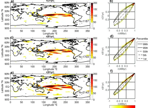
– The first version represents the scenario where all pseudoproxies with a good cor-relation, defined as|r| ≥0.3, over the whole time period (499 years long) can be used in the reconstructions Fig. 1b. This can be conceptualised by using Fig. 1a, with this series corresponding to selecting the areas where|r|>0.3 on thexaxis (wherer is 499 year correlation). Information from the entire time series is

avail-5

able in this scenario, and can be thought of using a calibration window 499 years long.

– The second version represents the realistic scenario, where calibration informa-tion is restricted to within a relatively small window and the long term correlainforma-tion is unknown, much like the eﬀ_{ects of limited instrumental data in reality. This can be}

10

thought of selecting the areas where|r|>0.3 on they axis (wherer is correlation in the calibration window). This implies that there is a chance that the mean corre-lation over the whole time series is zero, or perhaps the opposite to the expected sign, and this is when non-stationarities are likely to be the largest problem for re-constructions. This would vary with calibration window, and is reflected in Fig. 2b,

15

d and f, with the narrowing of the percentile lines as the length of the calibration window increases.

– The third version represents a combination of the first two series, selecting the proxies with a good correlation in the calibration window, but also over the whole time period (which would normally be unknown). This is equivalent to the case

20

where a proxy is selected during a calibration period, but also happens to have good correlations outside the window – the ideal proxy. This is represented by the overlapping areas of the first two series in Figs. 1a, and 2b, d and f for corre-sponding window lengths. This scenario uses a small calibration window like the second version of experiments, but uses information from the 499 years of data

25

as an additional more stringent pseudoproxy selection criterion.

(11)

calibra-CPD

11, 3853–3895, 2015

R. Batehup et al.

Title Page

Tables Figures

◭ ◮

Back Close

Full Screen / Esc

Discussion

P

a

per

|

Discussion

P

a

per

|

Discussion

P

a

per

|

Discussion

P

a

per

|

tion windows and using information about the long term strength of teleconnections re-sults in more robust reconstructions. However, in reality, the generation of paleoclimate reconstructions would apply an assumption equivalent to that of the second version of experiments, which limit the information on teleconnection strength to the calibration period only as they are constrained by the instrumental record. However, our

experi-5

ments showed that this assumption also produces larger errors in the reconstruction (not shown).

For the remainder of the paper, we show the second version of the experiments only, as it represents the most realistic case. For each grid-box, the 499 year time series was split into ten calibration windows, of lengths 31, 61 and 91 years to match the

run-10

ning correlations performed previously. The mid-point of the calibration windows were spaced evenly in the 499 year dataset, regardless of the amount of overlap or gap be-tween them. Experiments were repeated for the diﬀ_{erent calibration window lengths}

and positions, so that the sensitivity of reconstruction skill to calibration window char-acteristics could be examined. This resulted in ten thousand reconstructions for each

15

calibration window length, for each experiment. The experiments based on pseudo-proxy selection are described in Sect. 4.

3.2 Identifying non-stationarities

This study examines the conditions when non-stationary teleconnections impact the validity of paleoclimate reconstructions. Therefore it is necessary to identify which grid

20

points have non-stationary teleconnections, so that its impact on the reconstruction of ENSO can be assessed. The strength and variability of a location’s relationship with ENSO was measured by calculating the running correlation between the grid point TS or precipitation time series, and the modelled Niño 3.4 index. Running correlations used windows of 31, 61 or 91 years, in order to examine multidecadal scale variations

25

on a number of time scales.

(12)

run-CPD

11, 3853–3895, 2015

R. Batehup et al.

Title Page

Tables Figures

◭ ◮

Back Close

Full Screen / Esc

Discussion

P

a

per

|

Discussion

P

a

per

|

Discussion

P

a

per

|

Discussion

P

a

per

|

ning correlations from the GFDL CM2.1 were stationary. For this purpose, the running correlations computed from the GFDL CM2.1 were compared to the expected range of variation that the running correlations would exhibit if they were influenced by random noise (e.g. weather events) at the grid point location only. A Monte Carlo approach (sim-ilar to van Oldenborgh and Burgers, 2005; Sterl et al., 2007; Gallant et al., 2013) was

5

used to generate stochastic simulations of TS and precipitation data at each grid point. The simulated data were constructed to have the same statistical attributes as the TS and precipitation data from the GFDL CM2.1 simulation. One thousand stochastic time series were computed for each grid point in order to determine this range, according to the following equation from Gallant et al. (2013).

10

υ(t)=_a₀+_a₁_c₍_t₎+_σ

υ p

1−r2_[_η

υ(t)+Bηυ(t−1)] (1)

υ(t) is the stochastic TS or precipitation time series. The first two terms represent the stationary teleconnection strength, witha0anda1the regression coeﬃcients between

the grid point temperature or precipitation and the Niño 3.4 indexc(t). The other terms represent the added noise. A red noise process η_υ(t)+_Bη

υ(t−1), was used and is

15

weighted by the standard deviationσυof the local TS or precipitation time series, and the proportion of the regression’s unexplained variancep1−r2_(where_r _{is correlation}

of the local time series to the Niño 3.4 index). The red noise is generated by the sum of Gaussian noise (ηυ) and autocorrelation (B) of the TS or precipitation time series at lag of 1 year.

20

A 95 % confidence interval was generated at each grid point from the stochastic simulations and was used to represent the range of running correlations possible, as-suming a teleconnection was stationary. Thus, if a running correlation from the GFDL CM2.1 fell outside the range from the stochastic simulations, it was unlikely to have been influenced by stochastic processes alone. Hence, the teleconnection is defined

25

(13)

CPD

11, 3853–3895, 2015

R. Batehup et al.

Title Page

Tables Figures

◭ ◮

Back Close

Full Screen / Esc

Discussion

P

a

per

|

Discussion

P

a

per

|

Discussion

P

a

per

|

Discussion

P

a

per

|

false-positives in the time series of running correlations a grid point was defined as non-stationary only if the model running correlation time series fell outside the 95 % confi-dence interval more than 10 % of the time, which is double than expected by chance alone. As correlations are bounded, the running correlations were converted to Fisher Z scores using the following equation.

5

Z=₁_/_{2 ln[(1}+_r₎_/₍₁₋_r_)] ₍₂₎

Z is the Fisher Z score, whiler is the running correlation values.

Figure 2a, c and e shows the number of non-stationary years identified in the TS time series at each grid point for the diﬀ_{erent running correlation windows. Note that}

the points classified as non-stationary are denoted by the coloured areas in panels

10

a, c, and e, while white areas indicate stationary teleconnections. There are more non-stationary grid points (N value on plot) with larger running correlation windows, suggesting that non-stochastic influences on teleconnections increase as time scales increase. Of further note is a large non-stationary area in the equatorial Pacific, given this is the area surrounding our ENSO index it is debatable whether this should be

15

considered as a non-stationarity. Rather, we expect the changing relationship in this surrounding region to be the result of ENSO’s non-linearities (An and Jin, 2004) and/or changes in its spatial structure (CP-EP type events) which may be considered diﬀ

er-ent flavours of ever-ents rather than non-stationarity teleconnections of the ever-ent (Gallant et al., 2013; Sterl et al., 2007).

20

3.3 Reconstruction methods

This study examines the likely eﬀ_{ects of non-stationarities on multi-proxy}

reconstruc-tions of the running variance of the Niño 3.4 index (representing the variability of ENSO) using pseudoproxy data. Four simple, commonly-used multi-proxy reconstruction meth-ods were selected. In some methmeth-ods, such as composite plus scaling (CPS), there are

25

(14)

CPD

11, 3853–3895, 2015

R. Batehup et al.

Title Page

Tables Figures

◭ ◮

Back Close

Full Screen / Esc

Discussion

P

a

per

|

Discussion

P

a

per

|

Discussion

P

a

per

|

Discussion

P

a

per

|

et al., 2009). However, the impact of non-stationarity on these will not be examined in this study. The reconstruction methods to be tested are as follows:

3.3.1 Median Running Variance (MRV) method

The MRV method was developed by McGregor et al. (2013) to reconstruct the running variance of paleo-ENSO from climate proxy data. It involves calculating the running

5

variance of each of the normalised (zero mean and unit variance) proxy time series, and then calculating the median of these time series. The selected proxies have a demon-strated link to ENSO, identified by a correlation above the prescribed value, to ensure the resulting median time series contains information about ENSO variability.

3.3.2 Running Variance of Median (RVM) method

10

This method was also devised by McGregor et al. (2013), as an alternate to the MRV for calculating ENSO running variance. Here, if the constituent pseudoproxy series is negatively correlated to Nino 3.4, it is flipped in sign before being used for calculations. Each of the proxy time series are normalised to zero mean and unit variance before the median of the group is calculated. This median time series is then normalised prior to

15

calculating its running variance, which is the RVM reconstruction. Despite only diﬀ_ering

in the order of operations with the MRV, this method was included in the study as it uses raw time series data, rather than pre-processed data as for the MRV method.

3.3.3 Composite Plus Scaling (CPS) method

CPS is a common method for reconstructing climate data from climate proxies (Esper

20

(15)

CPD

11, 3853–3895, 2015

R. Batehup et al.

Title Page

Tables Figures

◭ ◮

Back Close

Full Screen / Esc

Discussion

P

a

per

|

Discussion

P

a

per

|

Discussion

P

a

per

|

Discussion

P

a

per

|

After normalising this single time series, running variance is taken to reconstruct ENSO variance, hereafter called “CPS_RV”.

3.3.4 Empirical Orthogonal Function Principal Component (EPC) method

This method, described in detail in Braganza et al. (2009), is based on the ability of Empirical Orthogonal Functions (EOFs) to extract the leading modes of variability from

5

a dataset (Xiao et al., 2014, and references therein). Like the MRV method, the proxy data must have established connections to ENSO to ensure that the common dominant signal is an ENSO signal. The leading EOF is then multiplied by the original pseudo-proxies, and summed to produce a principal component (PC) time series that is a re-construction of the ENSO index. The sign of the leading EOF is flipped, if necessary,

10

to ensure that the resulting PC has a positive correlation with the modelled ENSO. Like the CPS method, the running variance of this normalised PC time series is calculated to produce a reconstruction of ENSO variance (hereafter named “EPC_RV”).

3.4 Reconstruction performance

To measure the skill of the reconstructions, each are quantitatively compared to the

15

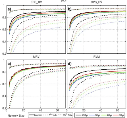
running variance of the ENSO index in the model (calculated in Sect. 2) by calculating Pearson correlation coeﬃ_{cients and root-mean-squared error (RMSE). Figure 3 shows}

that each of these four methods capture the running variance well when the entire dataset is available (with larger proxy networks). Therefore, these methods can be viewed as eﬀ_{ective in performing climate reconstructions of ENSO variance. Using all}

20

(16)

CPD

11, 3853–3895, 2015

R. Batehup et al.

Title Page

Tables Figures

◭ ◮

Back Close

Full Screen / Esc

Discussion

P

a

per

|

Discussion

P

a

per

|

Discussion

P

a

per

|

Discussion

P

a

per

|

4 Results

The results of the pseudoproxy experiments are presented in this section. Calibration windows of 31, 61 or 91 years are used to generate the reconstructions, and this win-dow length also corresponds to that used for the running correlation. Only grid points with a good correlation to ENSO (>0.3) within the given calibration window were used

5

as pseudoproxies. Here we examine the sensitivity of the reconstruction methods to non-stationarities, and the eﬀ_{ect of proxy location on reconstruction skill. As stated}

previously, there will be a focus on the reconstructions produced using grid point TS as the pseudoproxies.

4.1 Proxy location effects

10

ENSO reconstructions are thought to be aﬀ_{ected by the locations of the constituent}

proxies, with many viewing proxies from within the tropical region with higher regard than those sourced elsewhere. These proxies are closest to the centre-of-action and thus expected to be more skilful. Here we examine the impact of tropical Pacific region proxies on reconstructions by comparing two experiments; RNDglb_ts which selects n

15

pseudoproxies randomly from the global domain (see Supplement Fig. 1 for locations), while RND_{ntrop_ts} has similar random selection but excluding the tropical region: 10◦S to 10◦N, 100 to 300◦E (RNDntrop_ts). Note that both experiments do not discriminate

between stationary and non-stationary locations in this section.

The reconstruction skill, which is represented by the correlation between the

pseu-20

doproxy reconstruction of the Niño 3.4 index from the pseudoproxy grid points and the model Niño 3.4 index, of both experiments is presented in Fig. 4. Here, network sizenis varied from three to 70 (described in Sect. 3.1) on thex axis of each panel, while rows represent the diﬀ_{erent sized calibration windows and columns the di}ﬀ_erent

reconstruction methods (see Sect. 3.3). Looking at the percentile range (Fig. 4,

shad-25

(17)

CPD

11, 3853–3895, 2015

R. Batehup et al.

Title Page

Tables Figures

◭ ◮

Back Close

Full Screen / Esc

Discussion

P

a

per

|

Discussion

P

a

per

|

Discussion

P

a

per

|

Discussion

P

a

per

|

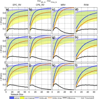
These diﬀ_{erences are most easily highlighted by arbitrarily defining skilful}

structions by some threshold and calculating what proportion of experiment’s recon-structions can be classified as skilful. Here we define skilful reconrecon-structions as those that explain more than half the variance of the model ENSO variability (grey line at∼0.7 correlation). The skill metrics for the global RNDglb_ts and non-tropical RNDntrop_ts

ex-5

periments, which are respectively plotted in each panel of Fig. 4 as blue and orange lines, can then be further simplified by focusing on the skill diﬀ_{erence between}

exper-iments (Fig. 4, black line). The skill diﬀ_{erence shows clear calibration window length}

and reconstruction method diﬀ_{erences that will be discussed further in Sect. 4.3, but}

on average when tropical proxies are not used in reconstructions, the proportion of

10

skilful reconstructions decreases by 14 %. However, even without the tropical proxies, the RNDntrop_ts experiment still produced quite high proportions of skilful

reconstruc-tions for larger network sizes. This implies that although there is a reduction in skill with extra-tropical proxies, non-tropical reconstructions still have a high likelihood of producing skilful reconstructions.

15

4.2 E_ffect of non-stationarities

Here we examine the eﬀ_{ect of non-stationarities on reconstructions of ENSO in order}

to understand how they may impact past reconstructions of ENSO variability. To this end, we compare the results of two experiments; (i) STATntrop_ts, which selects

pseu-doproxies from the same region as RNDntrop_ts but only includes pseudoproxies that

20

are considered stationary (see definition in Sect. 3.2), while (ii) NSTAT_{ntrop_ts} selects from the same region, but only the non-stationary pseudoproxies. Thus, here we ef-fectively separate the psuedoproxies of the RNDntrop_ts experiment into stationary and

non-stationary subgroups and generate reconstructions from each.

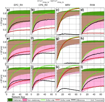
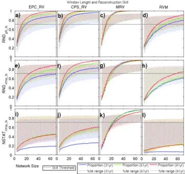
Figure 5 has the same panel layout as Fig. 4, with the green and pink

represent-25

ing stationary (STATntrop_ts) and non-stationary (NSTATntrop_ts) experiments. Shading

(18)

CPD

11, 3853–3895, 2015

R. Batehup et al.

Title Page

Tables Figures

◭ ◮

Back Close

Full Screen / Esc

Discussion

P

a

per

|

Discussion

P

a

per

|

Discussion

P

a

per

|

Discussion

P

a

per

|

the stationary (STAT_{ntrop_ts}) and non-stationary (NSTAT_{ntrop_ts}) experiments. In all cal-ibration window lengths (rows) and reconstruction methods (columns), the stationary experiment has greater skill than the non-stationary experiment, although there is rea-sonable variation between reconstruction methods and calibration window lengths (this will be discussed in later sections). In some cases, non-stationarities can reduce the

5

proportion of skilful reconstructions by up to 60 % (panel b, black line, n >60), but on average the proportion of skilful reconstructions is reduced by 30 %. Thus, these experiments suggest that extra-tropical non-stationarities act to reduce reconstruction skill.

It is interesting to note that when tropical region non-stationarities are included, they

10

appear to improve reconstruction skill (Supplement Fig. S4). The majority of the pseu-doproxies in the tropical region were found to be highly correlated with ENSO as expected, and to demonstrate very little variation in their correlations to ENSO (not shown), usually less than∼0.1 correlation. However, as seen in Fig. 2 many of these proxies are still classified as non-stationary, which may be due to non-linearities or

vari-15

ations in flavour of ENSO events. Thus, regardless of whether they are classified as non-stationary or not, the inclusion of these tropical pseudoproxies acts to improve the skill of the ENSO reconstructions.

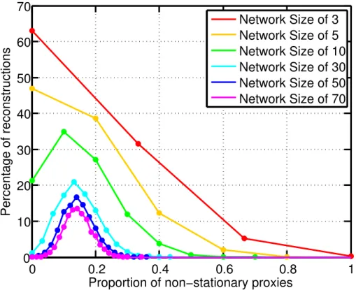
In regards to why non-stationarities do not seem to impact the high skill of ran-dom pseudoproxy selection of Sect. 4.1, we find that the likelihood of selecting

non-20

stationarities is relatively low. For instance, Fig. 6 shows the proportions of non-stationary pseudoproxies in the reconstructions for the RNDglb_ts experiment with

a 31 year long calibration window. It varies with diﬀ_{erent proxy network sizes, but as}

expected, the smaller groups have a greater chance of higher proportions of non-stationary proxies. With networks greater than thirty, the most likely proportion is

25

around 14 %, while much more consistent than the smaller groups. Even with very small group sizes (n=_{3), the chance that all stations are non-stationary is only 0.3 %}

(red line from Fig. 6). When only using extra-tropical locations (RNDntrop_ts), the most

(19)

CPD

11, 3853–3895, 2015

R. Batehup et al.

Title Page

Tables Figures

◭ ◮

Back Close

Full Screen / Esc

Discussion

P

a

per

|

Discussion

P

a

per

|

Discussion

P

a

per

|

Discussion

P

a

per

|

of all constituent proxies being stationary. There is also a tendency for more non-stationarities to occur with the use of longer calibration windows (see Fig. 2a), con-sequently the proportions of non-stationary proxies increase. For example, networks greater than thirty proxies can be up to 25 % non-stationary when using 91 year cal-ibration windows (not shown). Regardless of the increases in non-stationarities with

5

the use of longer calibration windows, these longer windows still produced more skilful reconstructions in the random selection experiments than those with shorter windows (RNDglb_tsand RNDntrop_ts; Fig. 4). Thus, although non-stationarities have the potential

to influence the skill of ENSO reconstructions, this scenario appears unlikely if proxies are selected similar to a globally random manner.

10

However, if pseudoproxies are selected from regions that have non-stationarities occurring at the same time, reconstruction skill is devastated. To this end, an Empir-ical Orthogonal Function analysis (EOF) was essentially used to “organise” the non-stationarities, resulting in the experiment PNEOF1 in Fig. 7. In this experiment the EOF was carried out on the running correlations between TS and Niño 3.4 SST anomalies at

15

each grid point. Pseudoproxy networks were then selected only from those grid points that exhibited a strong relationship with the leading EOF (i.e. the absolute value of the EOF weighting >0.1). The spatial map of this leading EOF is shown in panel e, for 31 year window running correlations. The leading EOFs of the longer windows have very similar spatial patterns, with spatial correlations of 0.86 and 0.84 produced

re-20

spectively, when comparing the 61 and 91 year window length EOF1 spatial patterns (not shown). The leading principal components for each window length are also similar (panel f). The resulting PNEOF1 experiment reconstructions display a large loss in skill when compared to the stationary pseudoproxies in the reconstructions (STATntrop_ts,

dashed lines), with the former having very little likelihood of producing a skilful

recon-25

struction (Fig. 7a). This highlights that non-stationarities can significantly aﬀ_{ect the skill}

(20)

CPD

11, 3853–3895, 2015

R. Batehup et al.

Title Page

Tables Figures

◭ ◮

Back Close

Full Screen / Esc

Discussion

P

a

per

|

Discussion

P

a

per

|

Discussion

P

a

per

|

Discussion

P

a

per

|

4.3 Pseudoproxy network size and length

As shown previously, the ENSO reconstruction skill is sensitive to the pseudoproxy network size and window length. This is clearly seen in Fig. 8, which displays the reconstruction skill of three diﬀ_{erent previously presented experiments (RND}

glb_ts,

RNDntrop_ts, and NSTATntrop_ts). In each panel the three colours indicate which

calibra-5

tion window length is used; 31 (blue), 61 (green), or 91 (red) years, while the hatching is the percentile range, and the thick lines are the proportion of skilful reconstructions. What is clear in all panels, is that the reconstruction skill generally improves with in-creasing network size for all experiments, that is regardless of reconstruction method and calibration window length. This is also true when all pseudoproxies in a network

10

are non-stationary (NSTATntrop_ts experiment), however, the reconstruction skill

gen-erally improves at a slower rate (Fig. 8i, j, l) . This implies that larger pseudoproxy networks are less aﬀ_{ected by non-stationarities, but this is also dependent on the}

cali-bration window length (discussed below) and the reconstruction method (discussed in Sect. 4.4). In general, smaller pseudoproxy networks (<5) produce very low

propor-15

tions of skilful reconstructions (10–40 %), while those with larger networks the majority of reconstructions become skilful. In fact, when pseudoproxies are randomly selected (RNDglb_ts and RNDntrop_ts), using a minimum of 20 proxies gives a fairly good chance

(>77 % chance on average) that the resulting reconstruction will be skilful (Fig. 8a–c, e–g).

20

The calibration window length also has an impact on reconstruction skill and sen-sitivity to non-stationarities (Fig. 9). For example, using small calibration windows (31 to 91 years) compared to the total number of model years available (499 years) leads to a relative decrease in skill, as indicated by the black 499 year reconstruction being higher in skill than the reconstructions using smaller windows. This decrease of skill

25

(21)

CPD

11, 3853–3895, 2015

R. Batehup et al.

Title Page

Tables Figures

◭ ◮

Back Close

Full Screen / Esc

Discussion

P

a

per

|

Discussion

P

a

per

|

Discussion

P

a

per

|

Discussion

P

a

per

|

performing reconstruction method. Thus, although there is a reduction in skill due to loss of information with smaller calibration window lengths, this is relatively small com-pared to the possible impacts of non-stationarities (see previous section). Figure 8 also shows that larger windows tend to improve skill, with the larger window lengths consistently having higher proportions of skilful reconstructions in the random

selec-5

tion experiments (RNDglb_tsand RNDntrop_ts). Larger windows also appear to generally

improve reconstructions in the NSTAT_{ntrop_ts} experiment. However, for random proxy selection, longer calibration windows still lead to increases in reconstruction skill, as long as the proxy network is not entirely non-stationary (like in the NSTATntrop_ts

ex-periment). This increase in skill is not as great as removing non-stationarities from the

10

reconstructions (Fig. 5) or changing the reconstruction method (following section).

4.4 Reconstruction method comparison

All reconstruction methods create skilful reconstructions given suﬃ_{ciently large}

calibra-tion windows and proxy network sizes in the random seleccalibra-tion experiments RND_{glb_ts} and RNDntrop_ts (see Figs. 8 and 9). It is noted that the CPS_RV method performs

15

well, although mainly with longer calibration windows and for the random selection ex-periments (RND_{glb_ts} and RND_{ntrop_ts}, Fig. 8). However, there is a clear distinction in the skill from the MRV method reconstructions compared to the other methods tested when considering the impact of non-stationarities and neglecting tropical pseudoprox-ies. For instance, when tropical pseudoproxies are not used in experiments, the MRV

20

reconstructions are only marginally aﬀ_{ected (Fig. 4c, g and k) implying that the method}

is not as dependent as other methods on the highly correlated tropical region. This is expected, as the EPC_RV and CPS_RV involve weighting regimes that would favour the highly correlated tropical pseudoproxies (see Sect. 3.3, and references therein). The MRV method has the highest proportion of skilful reconstructions at the lowest

25

network sizes in all other experiments (Fig. 8), with the clearest diﬀ_{erences seen in}

(22)

CPD

11, 3853–3895, 2015

R. Batehup et al.

Title Page

Tables Figures

◭ ◮

Back Close

Full Screen / Esc

Discussion

P

a

per

|

Discussion

P

a

per

|

Discussion

P

a

per

|

Discussion

P

a

per

|

the lowest sensitivity to non-stationarities. Further to this, in spite of the MRV method being negatively aﬀ_{ected in the PNEOF1 experiment (Fig. 7, thick lines), and displaying}

some sensitivity to calibration window length (red line outperforms others), it produces the highest proportion of skilful reconstructions and is thus still the most robust against non-stationarities.

5

It is worth noting that although the MRV method shows the most consistently high correlations to ENSO, this high skill is not necessarily reflected in the RMSE (root-mean-square error). The RMSE of the MRV method is still the most consistent however (smallest percentile ranges, Supplement Fig. 5), but shows somewhat greater error than the other methods in this experiment (RND_{ntrop_ts}). MRV in the non-stationary

ex-10

periment (NSTAT_{ntrop_ts}, Supplement Fig. S6; PNEOF1, not shown) have similar RMSE values to other methods, likely due to the other methods gaining additional errors due to increased non-stationarities. Upon further inspection it is clear that the higher cor-relations of the MRV method are oﬀ_{set by the resulting running variance time series}

being much more damped than those of the other methods, which explains the high

15

RMSE error. This can be seen in Supplement Fig. S7, where the variance is taken of the reconstructions instead of the correlations like in previous analyses. The MRV results clearly show much lower variance than all the other methods (panels c, g and k), particularly at larger pseudoproxy network sizes, whilst the variance of other meth-ods remain relatively high with increasing network size. Due to the nature of the other

20

methods, they are normalised after the reconstruction but prior to the calculation of the running variance (see Sect. 3.3), while the MRV is not. Thus, while the MRV repro-duces ENSO variance with the highest skill, the MRV method may require re-scaling to better match the magnitude of the variance changes.

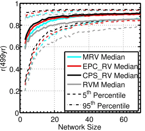
Given that the RVM and MRV methods are only diﬀ_{erent in order of operations (see}

25

Sect. 3.3) their large diﬀ_{erences in reconstruction skill suggest that using the median,}

(23)

suscep-CPD

11, 3853–3895, 2015

R. Batehup et al.

Title Page

Tables Figures

◭ ◮

Back Close

Full Screen / Esc

Discussion

P

a

per

|

Discussion

P

a

per

|

Discussion

P

a

per

|

Discussion

P

a

per

|

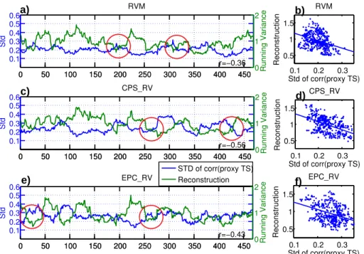
tible to signal cancellation like the other methods including the RVM. Thus, we sug-gest that the MRV method is robust against non-stationarities because they act much like dating errors and lead to signal cancellation. This is supported by Fig. 10, where a few examples of reconstructions are plotted alongside the standard deviation of their source pseudoproxies’ running correlation to model ENSO (see McGregor et al., 2013).

5

These plots suggest that when there is a lot of variability in the correlations between the source pseudoproxies and ENSO, the reconstruction variance tends to be low (and vice-versa), which can be seen in the red highlighted areas. This supports the idea that non-stationarities act to cancel the running variance signal much like a dating error. Further to this, the regressions of these individual time series also show the MRV’s

10

diﬀ_{erence to other methods, with a much smaller regression slope} ₋_{0.79 for MRV,}

compared to−2.28, −1.99 and −2.32 for the RVM, CPS_RV and EPC_RV methods, respectively (out of the statistically significant reconstructions). Thus, there is evidence that the MRV method is less prone to variance losses when there is high variability amongst the source proxies, and hence it is less susceptible to signal cancellation in

15

proxies.

4.5 Precipitation pseudoproxies

Although not the focus on this paper, precipitation was also examined for all experi-ments. Precipitation based reconstructions showed more variation in skill than TS and required larger network sizes for the same skill (see Supplement Fig. S2), but

other-20

wise had similar tendencies as temperature outlined above. However, there was one key diﬀ_{erence in precipitation – NSTAT}

glb_pr(Supplement Fig. S3) produced less skilful

reconstructions than RNDglb_pr(Supplement Fig. S2). This is likely due to the absence

of a large spatially coherent region of correlations in the tropical Pacific Ocean (see Supplement Fig. S1e). Generally, there is also greater variability in skill across

calibra-25

(24)

CPD

11, 3853–3895, 2015

R. Batehup et al.

Title Page

Tables Figures

◭ ◮

Back Close

Full Screen / Esc

Discussion

P

a

per

|

Discussion

P

a

per

|

Discussion

P

a

per

|

Discussion

P

a

per

|

method is generally unskilful, with the worst 5 % of reconstructions (blue shading) dis-playing correlations below zero with network sizes below 10 proxies. The RVM method appears to perform better with precipitation than temperature in panels d, and h, with not much diﬀ_{erence in panel l, which is consistent with the findings of McGregor et al.}

(2013).

5

5 Discussion

Non-stationary relationships between the modelled Niño 3.4 index and regional tem-perature and precipitation were detected in the GFDL CM2.1 model. Our results demonstrate that non-stationarities between ENSO and regional climates can occur in many regions around the globe, which extends previous work of Gallant et al. (2013),

10

who found significant non-stationary areas in the Australasian region in both modelling and observations. Like in Gallant et al. (2013), our work shows non-stationarities exist in climate models globally on time scales longer than approximately 30 years, demon-strating their occurrence at low frequencies. This is in contrast to van Oldenborgh and Burgers (2005) and Sterl et al. (2007), who examined non-stationarities at higher

fre-15

quencies and found no detectable evidence for them in the observations using run-ning correlation windows of around 20 years. The fact that these non-stationarities are found in a pre-industrial control simulation shows that this low frequency variability can arise from unforced, internal climate variability, adding further evidence that this low frequency variability is an inherent part of the climate system.

20

Identifying what causes the occurrence of non-stationarities in ENSO teleconnec-tions is not within the scope of this study. However, Wittenberg (2009) showed sub-stantial changes to the behaviour of ENSO on similar time scales to those identified here in a 2000 year simulation using the GFDL CM2.1. Wittenberg (2009) discussed that such changes to ENSO behaviour could conceivably alter the teleconnections

be-25

(25)

con-CPD

11, 3853–3895, 2015

R. Batehup et al.

Title Page

Tables Figures

◭ ◮

Back Close

Full Screen / Esc

Discussion

P

a

per

|

Discussion

P

a

per

|

Discussion

P

a

per

|

Discussion

P

a

per

|

figuration given that Gallant et al. (2013) identified non-stationarities in three diﬀ_erent

GCMs.

In this study, the pseudoproxy approach in the virtual reality of the GFDL CM2.1 pre-industrial control simulations avoids the problems of non-climate related noise that is inherent to real-world paleoclimate proxies, allowing us to focus on the sensitivity

5

of reconstructions to the occurrence of non-stationarities alone. However, in reality non-climate related sources of noise in paleoclimate proxies will confound, and likely degrade, reconstruction skill to a greater extent than examined here. Thus, our finding that a network size of>20 will minimise the eﬀ_{ects non-stationarities on reconstruction}

skill is likely an underestimate of minimum network size for a real-world reconstruction.

10

The compounding eﬀ_{ects of noise and non-stationarities on the reconstruction method}

and hence, a reconstruction, should be the focus of future research eﬀ_{orts in this area.}

All reconstruction methods examined generate skilful reconstructions when utilising globally random source proxy selection, given suﬃ_{ciently large calibration windows}

and proxy network sizes. Therefore, the results presented here highlight a case for

15

considering the influence of non-stationarities on real-world reconstructions, and their underlying methods, which generally employ small proxy networks. The influence of the choice of method on the reconstruction and its sensitivity to non-stationarities was stark. In the best-case scenario (i.e. long calibration window and large proxy network), the CPS_RV method had the greatest skill. In less-than-ideal conditions (e.g. small

cal-20

ibration windows or proxy networks), the MRV method clearly excelled, and even man-aged to produce a high proportion of skilful reconstructions given only pseudoproxies considered non-stationary (Fig. 5). However, note that the performance of these meth-ods is likely to depend on the variable being reconstructed. We also note that the large diﬀ_{erence between the MRV and RVM experiments (Figs. 3 and 9) is contradictory to}

25

the results in Fig. 4 of McGregor et al. (2013). However, these diﬀ_{erences were due to}

(26)

CPD

11, 3853–3895, 2015

R. Batehup et al.

Title Page

Tables Figures

◭ ◮

Back Close

Full Screen / Esc

Discussion

P

a

per

|

Discussion

P

a

per

|

Discussion

P

a

per

|

Discussion

P

a

per

|

For reconstructions of large-scale phenomena like ENSO, multi-proxy networks will produce more informative reconstructions because the larger networks contain more information, including spatial information, compared to single site (Mann, 2002; Lee et al., 2008; von Storch et al., 2009; McGregor et al., 2013). The experiments con-ducted here support this hypothesis, as the proportions of skilful reconstructions

in-5

crease for almost all reconstruction methods and calibration window lengths (Figs. 8 and 5). Our work further shows that large, multi-proxy networks also reduce errors re-lating to non-stationarity of teleconnections, which further supports their employment (Fig. 5). However, this skill improvement is aﬀ_{ected by the degree of non-stationarity}

present in the reconstructions, with non-stationary proxy networks (NSTAT_{ntrop_ts},

10

Fig. 8i–l) and “organised” non-stationarities (PNEOF1, Fig. 7a–d) reducing the degree of improvement in skill with increasing network size. Thus, where increasing network size would usually improve the reconstruction, non-stationarities can substantially tem-per this improvement. In extreme cases, where proxies are selected from areas with spatially coherent non-stationarities (PNEOF1, Fig. 7), reconstruction skill may show

15

no improvement with larger proxy networks. This further stresses the importance of ensuring that all constituent proxies utilised in a reconstruction are not aﬀ_{ected by the}

same non-stationarities. This is more likely achieved in spatially diverse, large multi-proxy networks.

The results of this study further emphasise the need for more paleoclimate proxies to

20

be available for multi-proxy climate reconstructions. Given the skilful reconstructions in ENSO variance that can be produced by neglecting pseudoproxies from the centre of action, as shown here, the utilisation of data solely from the eastern equatorial Pacific appears unnecessary. In fact, these results utilising globally random proxy selection support the development of paleoclimate proxies from a wide range of global locations.

25