Climate change impacts on maritime mountain snowpack in the Oregon Cascades

(1)

HESSD

9, 13037–13081, 2012

Climate change impacts on maritime mountain snowpack

E. Sproles et al.

Title Page

Abstract Introduction

Conclusions References

Tables Figures

◭ ◮

Back Close

Full Screen / Esc

Printer-friendly Version Interactive Discussion

Discussion

P

a

per

|

Dis

cussion

P

a

per

|

Discussion

P

a

per

|

Discussio

n

P

a

per

|

Hydrol. Earth Syst. Sci. Discuss., 9, 13037–13081, 2012 www.hydrol-earth-syst-sci-discuss.net/9/13037/2012/ doi:10.5194/hessd-9-13037-2012

Hydrology and Earth System Sciences Discussions

This discussion paper is/has been under review for the journal Hydrology and Earth System Sciences (HESS). Please refer to the corresponding final paper in HESS if available.

Climate change impacts on maritime

mountain snowpack in the Oregon

Cascades

E. Sproles1,*, A. Nolin1, K. Rittger2, and T. Painter2

1

College of Earth, Ocean, and Atmospheric Sciences, 104 CEOAS Administration Building, Oregon State University, Corvallis, OR, 97331-5503, USA

2

Jet Propulsion Laboratory, California Institute of Technology, 4800 Oak Grove Dr, Pasadena, CA, 91109, USA

*

currently at: National Health and Environmental Effects Research Laboratory, US Environmental Protection Agency, Corvallis, OR, USA

Received: 26 October 2012 – Accepted: 5 November 2012 – Published: 21 November 2012

Correspondence to: E. Sproles (eric.sproles@gmail.com)

(2)

HESSD

9, 13037–13081, 2012

E. Sproles et al.

Title Page

Tables Figures

◭ ◮

Back Close

Full Screen / Esc

Discussion

P

a

per

|

Dis

cussion

P

a

per

|

Discussion

P

a

per

|

Discussio

n

P

a

per

Abstract

Globally maritime snow comprises 10 % of seasonal snow and is considered highly sensitive to changes in temperature. This study investigates the effect of climate change on maritime mountain snowpack in the McKenzie River Basin (MRB) in the Cascades Mountains of Oregon, USA. Melt water from the MRB’s snowpack provides 5

critical water supply for agriculture, ecosystems, and municipalities throughout the re-gion especially in summer when water demand is high. Because maritime snow com-monly falls at temperatures close to 0◦C, accumulation of snow versus rainfall is highly sensitive to temperature increases. Analyses of current climate and projected climate change impacts show rising temperatures in the region. To better understand the sen-10

sitivity of snow accumulation to increased temperatures, we modeled the spatial distri-bution of snow water equivalent (SWE) in the MRB for the period of 1989–2009 with the SnowModel spatially distributed model. Simulations were evaluated using point-based measurements of SWE, precipitation, and temperature that showed Nash-Sutcli_ffe Ef-ficiency coefficients of 0.83, 0.97, and 0.80, respectively. Spatial accuracy was shown 15

to be 82 % using snow cover extent from the Landsat Thematic Mapper. The validated model was used to evaluate the sensitivity of snowpack to projected temperature in-creases and variability in precipitation, and how changes were expressed in the spatial and temporal distribution of SWE. Results show that a 2◦C increase in temperature would shift peak snowpack 12 days earlier and decrease basin-wide volumetric snow 20

water storage by 56 %. Snowpack between the elevations of 1000 and 1800 m is the most sensitive to increases in temperature. Upper elevations were also affected, but to a lesser degree. Temperature increases are the primary driver of diminished snowpack accumulation, however variability in precipitation produce discernible changes in the timing and volumetric storage of snowpack. This regional scale study serves as a case 25

(3)

HESSD

9, 13037–13081, 2012

E. Sproles et al.

Title Page

Tables Figures

◭ ◮

Back Close

Full Screen / Esc

Discussion

P

a

per

|

Dis

cussion

P

a

per

|

Discussion

P

a

per

|

Discussio

n

P

a

per

|

1 Introduction

1.1 Significance and motivation

The maritime snowpack of the Western Cascades of the Pacific Northwest (PNW), United States is characterized by temperatures near 0◦C throughout the winter and deep snow cover that can exceed 3000 mm (Sturm et al., 1995). This important compo-5

nent of the hydrologic cycle stores water during the winter months (November–March) when precipitation is highest, and provides melt water that recharges aquifers and sus-tains streams during the drier months of the year (June–September). Because maritime snow accumulates and persists at temperatures close to the melting point, it is funda-mentally at risk of warming temperatures (Nolin and Daly, 2006). The McKenzie River 10

Basin (MRB), located in the Central Western Cascades of Oregon, exhibits characteris-tics typical of many watersheds in this region, where maritime snowpack provides melt water for ecosystems, agriculture, hydropower, municipalities, and recreation – espe-cially in summer when demand is higher and precipitation reaches a minimum (United States Army Corps of Engineers, 2001; Oregon Water Supply and Conservation Initia-15

tive, 2008).

In the mountain West, snow water equivalent (SWE, the amount of water stored in the snowpack) reaches its basin-wide maximum on approximately 1 April (Serreze et al., 1999; Stewart et al., 2004). In the PNW, there have been significant declines in 1 April SWE and accompanying shifts in streamflow have been observed (Service, 2004; 20

Barnett et al., 2005; Mote et al., 2005; Luce and Holden, 2009; Stewart, 2009; Fritze et al., 2011). This reduction in SWE has been attributed to higher winter temperatures (Knowles et al., 2006; Mote, 2006; Abatzoglou, 2011; Fritze et al., 2011). Through-out the region, current analyses and those of projected future climate change impacts show rising temperatures (Mote and Salath ´e, 2010) which is expected to increasingly 25

(4)

HESSD

9, 13037–13081, 2012

E. Sproles et al.

Title Page

Tables Figures

◭ ◮

Back Close

Full Screen / Esc

Discussion

P

a

per

|

Dis

cussion

P

a

per

|

Discussion

P

a

per

|

Discussio

n

P

a

per

This problem is not unique to the Oregon Cascades and is of significance globally as snowmelt provides a sustained source of water for over one billion people (Bar-nett et al., 2005; Dozier, 2011). The maritime snow class comprises roughly 10 % of the spatial extent of all terrestrial seasonal snow (Sturm et al., 1995) and includes large portions of Japan, Eastern Europe, and the Western Cordillera of North America. Many 5

of these regions are mountainous, and measurements of snowpack are limited due to complex terrain and sparse observational networks. This deficiency limits the ability to accurately predict snowpack and runoffat the basin scale, especially in a changing cli-mate (Bales et al., 2006; Dozier, 2011). Improvements in quantifying the water storage of mountain snowpack in present and projected climates advance the ability to assess 10

climate impacts on hydrologic processes. While climate impacts on mountain snow-pack are a global concern, addressing them at the basin-level provides information at a scale that is effective for resource management strategies (Dozier, 2011).

Using the MRB as a case study that is representative of mid-latitude maritime snow-packs, this research examines and quantifies the sensitivity of snowpack to climate 15

change. Specifically the research objectives are to: (1) quantify the present-day dis-tribution of snow water equivalent; and (2) quantify the watershed-scale response of snow water equivalent to increases in temperature and variability in precipitation.

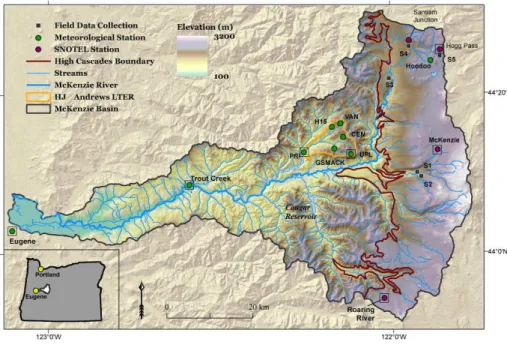
1.2 Study area

The McKenzie River Basin has an area of 3041 km2and ranges in elevation from 150 m 20

at the confluence with the Willamette River near the city of Eugene to over 3100 m at the crest of the Cascades. Precipitation increases with elevation in the MRB. Average annual precipitation ranges from approximately 1000 mm in the lower elevations to over 3500 mm in the Cascade Mountains (Je_fferson et al., 2008). With winter air tempera-tures commonly close to 0◦C, precipitation phase is highly sensitive to temperature and 25

(5)

HESSD

9, 13037–13081, 2012

E. Sproles et al.

Title Page

Tables Figures

◭ ◮

Back Close

Full Screen / Esc

Discussion

P

a

per

|

Dis

cussion

P

a

per

|

Discussion

P

a

per

|

Discussio

n

P

a

per

|

the fraction of total annual precipitation from snow is approximately 50 % (Jefferson et al., 2008). Here, deep snows accumulate from November through March, increasing their water storage until the onset of melt, about 1 April.

Stream discharge for the McKenzie River follows the seasonal precipitation pattern with a maximum in January (280 m3s−1, near Eugene) and a minimum of 62 m3s−1 in 5

September (United States Geological Survey, 2011b). Minimum flow can be explained by hydrogeologic properties that provide excellent aquifer storage (Tague and Grant, 2004; Je_fferson et al., 2008; Tague et al., 2008) and by the accumulation of a snowpack “reservoir” above 1200 m during the winter (Brooks et al., 2012). The MRB has two dis-tinct geologic provinces that further elucidate stream response to precipitation. The 10

older Western Cascades basalts are a highly dissected Miocene-age volcanic land-scape characterized by high drainage density and steep slopes that are hydrologically responsive to precipitation (Tague and Grant, 2004). The upper elevation portion of the basin is dominated by the High Cascades basalts, characterized by Pleistocene-age basalt flows that provide excellent aquifer storage and a poorly defined stream network 15

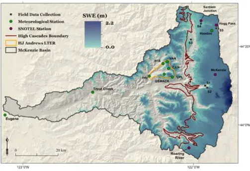
(Tague and Grant, 2004; Jefferson et al., 2008; Tague et al., 2008) (Fig. 1). The High Cascades are also characterized by deep snow accumulation and significant ground-water recharge that contribute to the MRB’s significant contribution to the late season discharge of the Willamette River. Using isotopic analysis, Brooks et al. (2012) found that 60–80 % of summer flow in the Willamette River originated from elevations over 20

1200 m in the Oregon Cascades. This upper elevation portion of the basin accounts for only 15.6 % of the annual precipitation in the Willamette River basin (Brooks et al., 2012).

The MRB is especially important as this watershed occupies 12 % of the Willamette River basin (30 300 km2), but supplies nearly 25 % of the late summer discharge at 25

(6)

HESSD

9, 13037–13081, 2012

E. Sproles et al.

Title Page

Tables Figures

◭ ◮

Back Close

Full Screen / Esc

Discussion

P

a

per

|

Dis

cussion

P

a

per

|

Discussion

P

a

per

|

Discussio

n

P

a

per

the Willamette River, especially in summer months when rainfall is sparse. This makes the MRB a key resource for ecological, urban, and agricultural interests and of great interest to water resource managers in the MRB and Willamette River Basin.

The present-day monitoring of mountain snowpack in the Western United States typically uses point-based data from the Natural Resources Conservation Service 5

(NRCS) Snowpack Telemetry (SNOTEL) network, supplying measurements of snow water equivalent, snowpack depth, air temperature, and cumulative precipitation. While measurements of snow have been conducted at the local scale for decades in the Oregon Cascades, accurate measurements of basin-wide mountain snowpack do not exist for the MRB or elsewhere on the planet (Dozier, 2011; Nolin, 2012). The SNO-10

TEL monitoring network is not representative of the spatial and temporal variability of SWE (Nolin et al., 2012). For instance, in the MRB the four monitoring sites cover an elevation range of only 245 m (1267–1512 m) in a basin where snow typically falls at el-evations between 750 and 3100 m. While these middle elel-evations are well represented, they do not quantify SWE at high elevations where over half of the snow-covered area 15

in the MRB is located above the elevation of the highest monitoring site (Nolin et al., 2012). Once the snow melts at the monitoring sites, there is no further information even though snow persists at higher elevations for several weeks. In the past, this limited configuration of SNOTEL sites has functioned successfully in helping predict streamflow (Pagano et al., 2004), however the network was not designed to monitor 20

climate change at the watershed scale (Molotch and Bales, 2006; Brown, 2009; Nolin et al., 2012) and, with continued warming, may no longer be effective for streamflow prediction.

A point-based monitoring network limits water managers’ ability to quantify and eval-uate the impacts of projected future climate change at the watershed scale. Previous 25

(7)

HESSD

9, 13037–13081, 2012

E. Sproles et al.

Title Page

Tables Figures

◭ ◮

Back Close

Full Screen / Esc

Discussion

P

a

per

|

Dis

cussion

P

a

per

|

Discussion

P

a

per

|

Discussio

n

P

a

per

|

vegetation (Hamlet and Lettenmaier, 2005). Results from Nolin et al. (2012) show that elevation and vegetation are the primary physiographic variable in determining SWE distributions in the MRB and Tague and Grant (2004) demonstrate the importance of geologic variability in determining groundwater recharge and streamflow in the Cas-cades. Thus, a watershed-scale understanding of SWE and water storage in the MRB 5

at higher resolution will be a valuable benefit to those managing this vital resource. Both spatially distributed snow models and remote sensing data can provide key information on spatially varying snow processes at the watershed scale. In the past decade, spatially distributed, deterministic snowpack modeling has made significant advances (Marks et al., 1999; Lehning et al., 2006; Liston and Elder, 2006a; Bavay 10

et al., 2009). These advances provide diagnostic information on relationships between physiographic characteristics of watersheds and snowpack dynamics. Such mechanis-tic snowpack models also allow us to make projections for future climate scenarios. Remote sensing is an e_ffective means of mapping the spatio-temporal character of seasonal snow (Nolin, 2011). Rittger (2012) used a computationally efficient method 15

to compute Fractional Snow Cover Area (fSCA) from Landsat Thematic Mapper (TM) (United States Geological Survey, 2011a) based on the work of Rosenthal and Dozier (1996) and Painter et al. (2009). Such data are at a spatial scale comparable to to-pographic and vegetation variations in the MRB and are appropriate for capturing the heterogeneous melt patterns in this watershed. By mapping fSCA, we can obtain an 20

accurate estimate of spatially and temporally varying snow extent, however these data cannot provide estimates of SWE.

2 Research methodology

The overall approach to addressing the research questions can be described in three general steps: (1) apply a physically based, spatially distributed model that uses mete-25

(8)

HESSD

9, 13037–13081, 2012

E. Sproles et al.

Title Page

Tables Figures

◭ ◮

Back Close

Full Screen / Esc

Discussion

P

a

per

|

Dis

cussion

P

a

per

|

Discussion

P

a

per

|

Discussio

n

P

a

per

a sensitivity analysis of snowpack with regard to temperature and precipitation. Each of these steps is described in greater detail below.

2.1 Modeling the snowpack

SnowModel (Liston and Elder, 2006a) was used to simulate meteorological and snow conditions throughout the McKenzie River Basin. SnowModel (Liston and Elder, 2006a) 5

is a spatially distributed, process based model that computes temperature, precipi-tation, and the full winter season evolution of SWE including accumulation, canopy interception, wind redistribution, sublimation/evaporation, and melt. SnowModel was selected because of its ability to simulate fine scale meteorological conditions in com-plex terrain at the watershed scale with a high degree of accuracy (Liston and Elder, 10

2006a). SnowModel has been successfully applied over a range of snow environments including Colorado, Antarctica, Idaho, Wyoming, Alaska, Greenland, Norway, and the European Alps (Liston and Elder, 2006a). SnowModel is composed of four sub-models: MicroMet, EnBal, SnowTran 3-D, and SnowPack. The MicroMet sub-model spatially distributes meteorological inputs to provide realistic distributions of air temperature, 15

humidity, precipitation, temperature, wind speed and wind direction, surface pressure, incoming solar and longwave radiation (Liston and Elder, 2006b). The EnBal sub-model computes the internal energy balance of the snowpack using atmospheric conditions computed by MicroMet (Liston and Elder, 2006a). The SnowTran 3-D sub-model is a physically-based snow transport model that distributes the transport and sublima-20

tion of snow due to wind (Liston et al., 2007). SnowPack is a single layer sub-model that calculates changes in snow depth and SWE from fluxes in precipitation and melt (Liston and Elder, 2006a). The model was run at daily time steps and at a grid res-olution of 100 m. These spatial and temporal resres-olutions are at a scale that captures the variability in topography and snowpack across the landscape while still retaining 25

(9)

HESSD

9, 13037–13081, 2012

E. Sproles et al.

Title Page

Tables Figures

◭ ◮

Back Close

Full Screen / Esc

Discussion

P

a

per

|

Dis

cussion

P

a

per

|

Discussion

P

a

per

|

Discussio

n

P

a

per

|

2.1.1 Model input data

SnowModel requires meteorological data as its fundamental input including air temper-ature, precipitation, relative humidity, wind speed, and wind direction. The simulations used meteorological data from seven automated weather stations distributed through-out the MRB at elevations ranging from 174 m to 1509 m (Fig. 1, Table 1). A spatially 5

balanced network of input stations was used to more evenly weight the forcing data across the watershed (Fig. 1 – stations used as model forcings are enclosed in a black square). The Barnes Objective Analysis technique, used in the MicroMet sub-model to distribute precipitation (P_{) and air temperature (}T_air_{), incorporates a weighted}

inter-polation scheme that is based on the data spacing from a datum (station) to the grid 10

cell (Koch et al., 1983). Although there are six stations in the HJ Andrews Experimen-tal Forest (HJA) (Daly and McKee, 2010) only two, Primary (PRI – 430 m) and Upper Lookout (UPL – 1294 m), were used to avoid overweighting of the central portion of the basin and for improved model calibration. Clusters of stations were found to negatively impact model results in the outer regions of the model domain. The addition of the Eu-15

gene Airport improved model agreement by providing a datum in the western portion of the basin. Trout Creek (Western Regional Climate Center, 2010) was added to more evenly distribute precipitation in the lower portions of the basin. The upper elevation SNOTEL (National Resource Conservation Service, 2010) sites were added to more evenly distribute meteorological conditions in the upper elevations. Stations were also 20

required to have a near-complete data record (greater than 90 %). Discussion on how this configuration was finalized is discussed in greater detail in the model calibration sub-section.

The period for this study, WY 1989–2009, was constrained by the availability of me-teorological data to drive the model. While all seven sites hadP _andT_air_{data, only PRI} 25

(10)

HESSD

9, 13037–13081, 2012

E. Sproles et al.

Title Page

Tables Figures

◭ ◮

Back Close

Full Screen / Esc

Discussion

P

a

per

|

Dis

cussion

P

a

per

|

Discussion

P

a

per

|

Discussio

n

P

a

per

period. This time period represents a warm phase of the Pacific Decadal Oscillation (Brown and Kipfmueller, 2012) and compared with records dating back 70 yr, SWE measurements are below the long-term mean (Nolin, 2012). A limited data set of hourly data for meteorological stations (10 yr) was available but because one of our goals was to model a relatively long time period, we selected the longer daily time series. Daily 5

mean values of temperature have a long data record; however the mean temperatures underestimated the amount of snow throughout all of the calibration years. SNOTEL sites in the MRB have temperature data recorded at 0 h (midnight), 6 h, 12 h, and 18 h throughout the reference period. We tested the model using temperature data from each of these times and achieved the most accurate model results when using data 10

acquired at midnight. This makes sense for several reasons. Temperatures at 12 h, and 18 h were too warm and so precipitation was partitioned as rain rather than snow. The pre-dawn 6 h temperatures were cold causing the model to overestimate the pro-portion of snowfall. The midnight temperature values provided the correct rain-snow partitioning in the model. Similarly, we found that using the midnight temperature data 15

allowed the model to better fit the melt patterns observed during the snow ablation period.

As boundary conditions, the model requires elevation and land cover for the model domain. Digital elevation data were obtained from the United States Geological Sur-vey’s (USGS) Seamless National Elevation Dataset (NED) (Gesch, 2007). The National 20

Land Cover Dataset (NLCD) (Fry et al., 2009) was also obtained through USGS. Both data sets were resampled from 30 m to the model grid resolution of 100 m resolution in ArcGIS 9.3 and using a nearest neighbor algorithm (ESRI, 2009). Concerns over po-tential misclassification of land cover that may arise from a nearest neighbor approach are moderated by landscape patterns in the areas where snowfall occurs. These areas 25

(11)

HESSD

9, 13037–13081, 2012

E. Sproles et al.

Title Page

Tables Figures

◭ ◮

Back Close

Full Screen / Esc

Discussion

P

a

per

|

Dis

cussion

P

a

per

|

Discussion

P

a

per

|

Discussio

n

P

a

per

|

forest landscape that includes active timber harvest and re-planting. However, devel-oping a dynamic land cover data set lies outside the scope of this research.

Resampling the 30-m data to a grid cell of 100 m captures variability in topography and snowpack across the landscape, while reducing the computational demands by a factor of eleven. The land cover boundary condition uses vegetation classes (i.e. 5

coniferous forest, farm land), so NLCD land cover types were reclassified to the appro-priate SnowModel land cover code (Sproles, 2012). The model domain was 112 km in the east–west direction and 76 km in the north–south direction. The file size of each daily model simulation for a single output (i.e. SWE, air temperature) was 9.7 MB. A sin-gle water year required approximately 200 min on a UNIX-operating system with 8 GB 10

of RAM and two dual-core AMD 64-bit processors.

2.1.2 Model modifications

Two primary modifications were made to SnowModel: a rain/snow precipitation partition function and an albedo decay function. These modifications more accurately simulate physical conditions, and improved model performance. The rain/snow precipitation par-15

tition function was required because in the maritime climate wintertime temperatures commonly remain close to 0◦C and mixed phase precipitation events are common. In the PNW, empirical measurements by the United States Army Corps of Engineers (USACE) (1956) show that the transition from rain to snow exists primarily between a temperature range of−2 to 2◦C. Based upon the USACE study the relationship was

20

implemented in the model using Eq. (2).

SFE=(0.25×(275.16−T_air))×P (1)

where, SFE (Snow Fall Equivalent) is the amount of amount of precipitation reaching the ground that falls as snow,T_air_{is air temperature, and}P _{is total precipitation. Rainfall}

is computed asP _{minus SFE.} 25

The shortwave albedo of snow (α_{) has significant e}_ff_{ects on surface energy}

(12)

HESSD

9, 13037–13081, 2012

E. Sproles et al.

Title Page

Tables Figures

◭ ◮

Back Close

Full Screen / Esc

Discussion

P

a

per

|

Dis

cussion

P

a

per

|

Discussion

P

a

per

|

Discussio

n

P

a

per

1980). New snow is highly reflective, with albedo greater than 0.8. However, snow albedo decays with time, which allows more incoming radiation to be absorbed. Snow albedo also declines faster in forested landscapes as forest litter is deposited and con-centrated at the snowpack surface (Hardy et al., 2000). This is pertinent in the maritime PNW as deep soils in the Western Cascades support dense forest while the High Cas-5

cades have poorly developed soils and a more open and often unforested landscape (Fig. 1).

Previous versions of SnowModel included snow albedo as a static, tunable param-eter (Liston and Elder, 2006a). This research applied improved snow albedo functions for forested and unforested areas that decay with time. This parsimonious approach 10

does not include the e_ffects of topography (Molotch et al., 2004). Following the work of Burles and Boon (2011), the maximum albedo value after new snowfall (when new snow depth ≥2.5 cm) is set to 0.8 in unforested areas and to 0.6 in forested areas (Burles and Boon, 2011). A minimum snow albedo (α_min) was set to 0.5 in unforested areas and 0.2 in forested areas. Albedo decay measurements in the study area did not 15

exist, thus the decay gradient for melting (grm) and non-melting (grnm) conditions were calibrated based on SWE measurements during the accumulation and ablation period. Albedo in the model decreases at each time step according to the following:

for non-melting conditions

α_t₌₍α_t₋₁−grnm) (2)

20

and, for melting snow

α_t₌₍₍α_t₋₁−α_min)×exp(−gr_m)+α_min (3)

Whereα_t₋₁_{represents the snow albedo at the previous time step, gr}_m₌_{0.018, gr}_nm₌

0.008, andα_tis the snow albedo value used at each time step by the model in energy balance calculations.

(13)

HESSD

9, 13037–13081, 2012

E. Sproles et al.

Title Page

Tables Figures

◭ ◮

Back Close

Full Screen / Esc

Discussion

P

a

per

|

Dis

cussion

P

a

per

|

Discussion

P

a

per

|

Discussio

n

P

a

per

|

2.1.3 Model calibration and assessment

Model calibration had two phases that carefully examined the accumulation and the ab-lation periods. The initial phase focused on optimizing the spatially-distributed gridded values of daily P and T_air. Because meteorological conditions are first order controls on snowpack accumulation and ablation, maximizing the accuracy of these spatially 5

interpolated and temporally varying model forcings is an important first step. Without accurate input, the resulting snowpack might be calibrated to correct values – but not for the right reasons (Kirchner, 2006). The second phase focused on optimizing the spa-tial extent of simulated snow with remotely sensed estimates. The optimal configuration of meteorological stations was determined by iteratively adding stations in the model. 10

Results of each iteration were compared to stations independent of those used in the model (Table 1) using metrics described below. Model evaluation used point-based measurements for SWE and the Landsat fSCA remote sensing data for snow cover ex-tent, providing a robust means of model calibration and validation (Bates, 2001). Paired water years of statistically high, low, and average peak SWE were used to calibrate and 15

validate the model (Table 2). Calibration was performed on the first set of water years, and then validated to the second set on water years. Once model calibration and vali-dation was completed for the selected years, the model was run for WY 1989–2009 to establish a present-day reference simulation for applying the future climate projections, and hereafter is referred to as the Reference period.

20

2.1.4 Calibration metrics

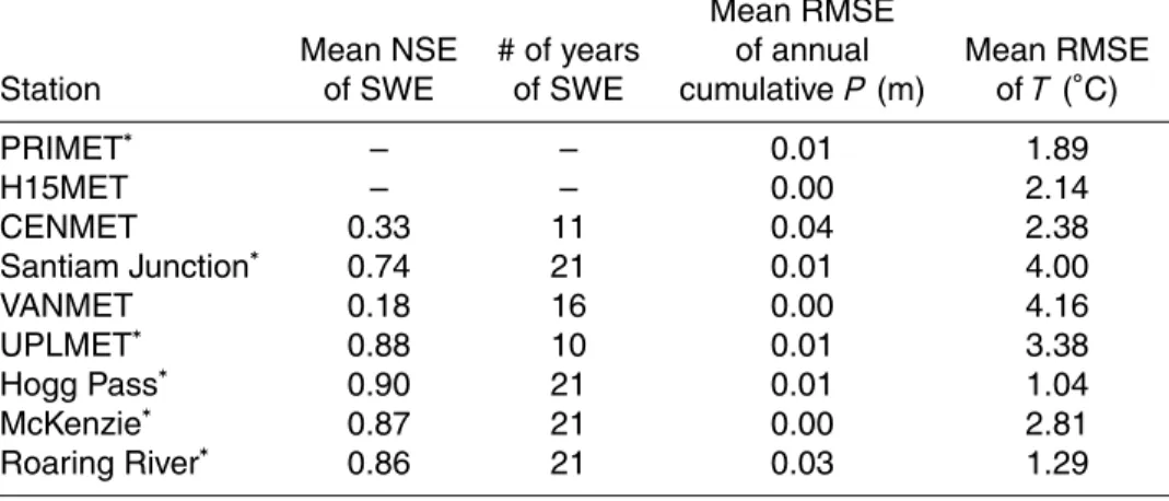
Nash-Sutcliffe Efficiency (NSE) and Root Mean Square Error (RMSE) were used to evaluate modeledP_,T_air_{, and SWE compared to measured values from SNOTEL}

sta-tions and meteorological stasta-tions independent of those used in the model. NSE is a dimensionless indicator of model performance where NSE=1 when simulations are 25

a perfect match with observations. For 0<_NSE<_{1, the model is more accurate than}

(14)

HESSD

9, 13037–13081, 2012

E. Sproles et al.

Title Page

Tables Figures

◭ ◮

Back Close

Full Screen / Esc

Discussion

P

a

per

|

Dis

cussion

P

a

per

|

Discussion

P

a

per

|

Discussio

n

P

a

per

(Moriasi et al., 2007), we used a target threshold of 0.80 or greater for all stations. This value represents a model e_fficiency that is very close to measured values and is significantly better than using mean values (Nash and Sutcliffe, 1970; Legates and Mc-Cabe, 1999). If NSE is less than 0, the mean is a better predictor (Nash and Sutcliffe, 1970; Legates and McCabe, 1999). RMSE indicates the overall di_fference between ob-5

served and simulated values, and retains the unit of measure (Armstrong and Collopy, 1992). RMSE provided a better understanding of the scale of error that occurred in simulations, and was used as a metric to improve model results.

Air temperature proved to be a challenging parameter to calibrate due to the complex terrain of the MRB. Here, true temperature lapse rates do not always follow a linear 10

temperature-elevation relationship and synoptic scale atmospheric patterns can a_ffect local lapse rates, especially when high pressure systems dominate causing cold air pooling (Daly et al., 2010). For the model, we used initial monthly lapse rates from the Washington Cascades, roughly 350 km north of the MRB (Minder et al., 2010). These lapse rates were iteratively adjusted to minimize RMSE for temperature using 15

the forcing and evaluation stations listed in Table 1. The final model iteration applied monthly lapse rate values ranging from 5.5–7◦C km−1 and were 1.5◦C km−1 cooler than Minder found in the Washington Cascades (Table 3). Minimum RMSE for some calibration sites were outside of the target threshold of 2◦C, as large errors for a few values can exacerbate RMSE values (Freedman et al., 1991). ThusR2_{values (Legates} 20

and McCabe, 1999) and 95 % confidence intervals were calculated (Freedman et al., 1991) to augment model evaluation. R2 _{values describe the proportion (0.0 to 1.0)}

of how much of the observed data can be described by the model, where a value of 1.0 is a perfect match with observed data. Confidence intervals indicate simulation reliability. Methods on how to potentially improve lapse rate calculations for future work 25

are described in the third paragraph of the Discussion section.

(15)

HESSD

9, 13037–13081, 2012

E. Sproles et al.

Title Page

Tables Figures

◭ ◮

Back Close

Full Screen / Esc

Discussion

P

a

per

|

Dis

cussion

P

a

per

|

Discussion

P

a

per

|

Discussio

n

P

a

per

|

month. Snow densities were calculated using monthly SWE measurements at five lo-cations in the basin. Four snow depth measurements were conducted within one meter of the initial SWE sample. This approach does not provide a detailed measurement of SWE in a 100 m×100 m grid cell, and thus was used as a broad metric for assessing

the magnitude of simulated SWE and the timing of accumulation and ablation. Logisti-5

cally, this rapid assessment approach allowed samples at all five sites to be conducted in a single day. In addition, colleagues at the University of Idaho provided SWE mea-surements at two locations in the basin on two dates in WY 2008 and 2009 (Link et al., 2010).

2.1.5 Remote sensing based calibration

10

The spatial extent of modeled snow cover was assessed using satellite-derived maps of fractional snow-covered area (fSCA). The Landsat TM fractional snow covered area data were aggregated from 30-m data to the 100-m grid resolution of SnowModel and converted to a binary grid where<_{15 % fSCA was classified as no snow, and}>_{15 %}

fSCA was classified as snow in the grid cell. The co-occurrence of modeled and mea-15

sured snow cover was assessed using metrics of accuracy, precision, and recall as in Painter et al. (2009). Precision is the probability that a pixel identified with snow in-deed has snow. Recall, the metric that Dong and Peters-Lidard (2010) employed, is the probability of detection of a snow-covered pixel. Accuracy is the probability a pixel is correctly classified. For detailed explanations of these measures and their application 20

to snow mapping, see Rittger et al. (2011).

There were a limited number of valid images each winter because of cloud cover and the 16-day repeat orbit. For example, during WY 2009, only one image between the months of November and April had a cloud cover less than 25 % in the MRB. However, each calibration year had at least one image with cloud cover less than 10 % that could 25

(16)

HESSD

9, 13037–13081, 2012

E. Sproles et al.

Title Page

Tables Figures

◭ ◮

Back Close

Full Screen / Esc

Discussion

P

a

per

|

Dis

cussion

P

a

per

|

Discussion

P

a

per

|

Discussio

n

P

a

per

and SnowModel results was evaluated for physiographic variables including land cover class, elevation, slope and aspect. This allows us to identify domain characteristics that were potentially misrepresented by the model.

2.2 Climate perturbations

The calibrated and validated model was run for the reference period and then used to 5

assess the sensitivity of snowpack to increased temperature and variable precipitation. To determine the response of snowpack to increased temperature and changes in precipitation, a sensitivity analysis was conducted in three phases. The first phase increased all temperature inputs for WY 1989–2009 by 2◦C (hereafter referred to by T2), which is considered to be the mean annual average temperature increase in the 10

region by mid-century (Mote and Salath ´e, 2010). The second and third phases retained the temperature increases, but also scaled precipitation inputs by±10 % to incorporate the uncertainty in projected future precipitation (Mote and Salath ´e, 2010). Hereafter these phases will be referred to by T2P10 (representing+2◦C and a 10 % increase in precipitation), and T2N10 (representing+2◦C and a 10 % decrease in precipitation). 15

Results from the±10 % precipitation also provide insight into how annual variability in precipitation can affect SWE relative to the effects of increased temperature. The model was then run, applying the three sets of scaled meteorological data for the reference period of WY 1989–2009.

3 Results

20

3.1 Model assessment

(17)

HESSD

9, 13037–13081, 2012

E. Sproles et al.

Title Page

Tables Figures

◭ ◮

Back Close

Full Screen / Esc

Discussion

P

a

per

|

Dis

cussion

P

a

per

|

Discussion

P

a

per

|

Discussio

n

P

a

per

|

reference stations (used to validate the model) (Figs. 2a, b). For years other than cal-ibration and validation years, the mean NSE ofP and T_air at all stations was 0.97 and 0.80 respectively (Table 4).

WY 1997 and 2005 were excluded from these metrics and in subsequent calculations discussed in this section. Evaluation of model results showed two unrelated problems 5

for these years. WY 1997 experienced at least 10 precipitation events>_{50 mm day}−1

during the winter months. Evaluation of the input data showed that in a few cases there were significant discrepancies (>1 m of annual cumulative precipitation) at several of the stations that were used as forcing data. Additionally, a few large precipitation inputs were offset by one day. The shifts were not systematic and appeared to be random in 10

nature, most likely due to equipment mistiming at several stations. As a result a storm with a significant amount of total precipitation (>_{50 mm) would, in e}_ff_{ect, be processed}

on two consecutive days by the model. While the errors were present in less than 10 % of the data sets, they occurred on days of heavy precipitation which magnified the error. While simulated distributed precipitation values for 1997 closely match the point-based 15

precipitation data used as input, there was a more than two-fold over estimation of SWE at all sites. Thus this year was omitted. WY 2005 displayed model deficiencies in resolving lapse rates associated with temperature inversions. Simulations of spa-tially distributed gridded temperature in WY 2005 had an RMSE and NSE of 3.8◦C and 0.72 respectively, whereas the reference period had values of 2.5◦C and 0.80. 20

This was due to extended periods of high pressure, which resulted in cold air pooling and negative temperature lapse rates (Daly et al., 2010). Extensive snowmelt and near complete loss of upper elevation snowpack occurred in mid-to-late February (National Resource Conservation Service, 2010) as unseasonably warm temperatures at higher elevations and unseasonably cool temperatures at lower elevations persisted for sev-25

eral weeks. The model deficiencies caused by such extensive temperature inversions are addressed in the Discussion section.

(18)

HESSD

9, 13037–13081, 2012

E. Sproles et al.

Title Page

Tables Figures

◭ ◮

Back Close

Full Screen / Esc

Discussion

P

a

per

|

Dis

cussion

P

a

per

|

Discussion

P

a

per

|

Discussio

n

P

a

per

mean NSE value was 0.96 for the full reference period. It is important to note that the addition of the low elevation Eugene Airport meteorological station greatly improved model performance. This station provided meteorological input data at a low elevation and at the western edge of the model domain, which improved the spatial interpolation of precipitation.

5

The mean RMSE was 2.5◦C and the mean NSE value was 0.80 (Fig. 2b and Ta-ble 4). Model simulations at the Santiam Junction SNOTEL station consistently un-derperformed in relation to all other stations. Santiam Junction is situated between an Oregon Department of Transportation facility and an airstrip. Thus, it lies at the west-ern edge of an exposed, flat plain that is physiographically dissimilar to its surroundings 10

and the other stations. There was an error forT_air that was consistent with regard to elevation. Simulations underestimatedT_air_{on average by 2.0}◦_{C at middle elevation}

sta-tions (800–1300 m). Steep slopes dominate the topography in this portion of the basin. The upper elevation stations (1300–1550 m) overestimated temperature on average by 0.25◦C. This bias reflects the topographic character of the MRB. The upper elevation 15

sites are situated in the High Cascades geological province, where the topography has a more gradual slope averaging approximately 10◦. In the Western Cascades geolog-ical province, slopes are steeper averaging approximately 20◦, but are also frequently characterized by slopes up to 50◦. In the Western Cascades during periods of high pressure, it is common to have cold air drainage, where cooler, more dense air moves 20

down a slope and pools in valleys creating cooler temperatures at lower elevations (Daly et al., 2010).

The RMSE for T_air (2.5◦C) was larger than anticipated, however further analysis showed an R2 _{of 0.85 and 98 % of all} T_air _{simulations within a 95 % confidence}

in-terval. The additional evaluation metrics support the probability that a small minority of 25

(19)

HESSD

9, 13037–13081, 2012

E. Sproles et al.

Title Page

Tables Figures

◭ ◮

Back Close

Full Screen / Esc

Discussion

P

a

per

|

Dis

cussion

P

a

per

|

Discussion

P

a

per

|

Discussio

n

P

a

per

|

in this study. Ideas on how to resolve these issues are found in the third paragraph of the Discussion section.

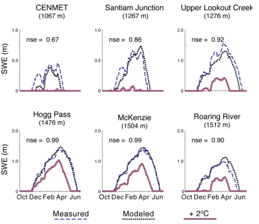
The model simulations of SWE (Figs. 3 and 4) showed mean NSE coefficients of 0.83 across the basin at point-based locations. The data record for SWE is more limited than the records ofP andT_air and only the four SNOTEL sites (elev. 1267 to 1512 m) 5

have measurements of SWE that span the full data record. These sites provide the primary reference points for model evaluation (Figs. 3 and 4). These elevations and the areas above accumulate the majority of SWE for the basin. Comparisons of observed and simulated values showed an RMSE of 0.13 m at all sites used in the validation SNOTEL sites (Table 4). It is worth noting the highest SNOTEL site is situated at an 10

elevation of 1512 m but 75 % of the model-estimated SWE lies above that elevation. This result is consistent with the work of Gillan et al. (2010) who found that>_{70 % of}

SWE accumulates above the mean elevation surrounding SNOTEL sites in a snow-dominated watershed in Northwestern Montana.

The length and consistency of the automated SWE data record at lower elevation 15

sites is more limited. With the exception of UPL, snow pillows in the HJA are not cal-ibrated and the reported data have not been fully quality assured. The result is an inconsistent dataset with values that often do not represent expected snowpack evo-lution in the region. Due to the questionable accuracy of the measured SWE values in the HJA, these data were not used as a metric for model validation. This issue also 20

highlights the need for a careful calibration and regular maintenance of SWE measure-ment sites. Field measuremeasure-ments collected during WY 2008 and 2009 were collected at a range of elevations and show a high level of agreement between measured and modeled SWE values.

In the spatial validation, 14-yr of SnowModel simulations of snow cover compared to 25

(20)

HESSD

9, 13037–13081, 2012

E. Sproles et al.

Title Page

Tables Figures

◭ ◮

Back Close

Full Screen / Esc

Discussion

P

a

per

|

Dis

cussion

P

a

per

|

Discussion

P

a

per

|

Discussio

n

P

a

per

Although the accuracy statistic may rise because of overwhelming numbers of cells in which there is no snow (Rittger et al., 2012), we include it because a large portion of the MRB can be snow covered and validation scenes are distributed throughout the season. Disagreement between the fSCA images and simulations primarily occurred where the model estimated snow cover and the fSCA did not have snow cover (13 %). 5

This degree of False Positive (FP) is expected as remotely sensed data typically omits snow cover in the steep and heavily forested landscapes that dominate the Western Cascades and the MRB (Nolin, 2011). The inter-annual changes associated with har-vested forest are not expressed in the static land cover dataset, but are incorporated into the fSCA product. This classification discrepancy propagated through each year 10

contributing to the lower precision value by decreasing the number of True Positive (TP). Additionally, the fSCA binary product classifies any cell with a fractional snow cover value less than 15 % as no snow. Even though the Landsat fSCA product was coarsened to 100 m, cells at the transitional snow line will be classified as no snow and result in an increase in False Positive (FP) classifications for modeled snow cover. WY 15

2006, 2008, and 2009 were the exceptions, showing more False Negative (FN) classi-fications, but with a similarly higher level of agreement. For a more detailed discussion of the model assessment using remote sensing data, please refer to Sproles (2012).

3.2 Impacts of warmer climate and changing precipitation on snow

3.2.1 Sensitivity of snowpack to changes in temperature and precipitation

20

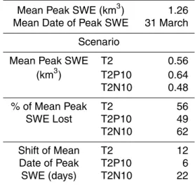
The response of snowpack in the MRB in the T2 scenario highlights the sensitivity to temperatures and that the greatest impact on SWE accumulation comes from more precipitation falling as rain rather than snow. Elevations below 1300 m show a sub-stantial loss of SWE accumulation (Fig. 3), where elevations around 1500 m suggest considerable losses of SWE, but still retaining a seasonal snowpack. Mean peak SWE 25

for the basin (the ±5-day mean from peak SWE) decreased by an average of 56 %

(21)

HESSD

9, 13037–13081, 2012

E. Sproles et al.

Title Page

Tables Figures

◭ ◮

Back Close

Full Screen / Esc

Discussion

P

a

per

|

Dis

cussion

P

a

per

|

Discussion

P

a

per

|

Discussio

n

P

a

per

|

the MRB, this equals an annual average loss of 0.70 km3 of water stored as snow – more than twice the volume the largest impoundment in the MRB (Cougar Reservoir, storage capacity 0.27 km3). While temperature is the controlling factor for the phase of precipitation and in turn changes in SWE, changes in total precipitation also have an impact. The T2P10 and T2N10 scenarios show losses of mean area-integrated peak 5

SWE of 0.62 to 0.78 km3, respectively, and reflect the role that precipitation variabil-ity plays on peak snowpack in the MRB. The 0.21 km3 difference of area-integrated peak SWE predicted by the T2P10 and T2N10 scenarios is substantial and is equal to slightly less than available storage at Cougar Reservoir. However 2◦C temperature increases alone result in a 0.70 km3loss (Fig. 6, Table 5). Increased precipitation in the 10

T2P10 scenario results in additional SWE at elevations primarily over 1800 m, mitigat-ing losses at those elevations. In these highest elevation portions of the basin a 2◦C increase in temperature is not sufficient to convert snowfall to rainfall or to significantly accelerate snowmelt. This increase in SWE at the high elevations partially offsets some of the losses at lower elevations.

15

With warmer conditions, the date of peak SWE is projected to occur earlier in the spring and properly into the winter (before the vernal equinox). The average date for simulated peak SWE in the MRB during the reference period is 31 March. However, in T2 the average date for peak SWE shifts 12 days earlier in the WY. Similarly, peak SWE arrives 6 days and 22 days earlier in the T2P10 and T2N10 scenarios, respectively 20

indicating a greater sensitivity in the T2N10 than the T2P10 scenario.

We assessed the sensitivity of the snowpack to temperature increases by elevation using the 10-day mean of peak SWE and frequency of snow cover for WY 2007. The 10-day mean of peak SWE minimized the influence of any single large accumulation event in order to emphasize the overall snowpack trend for that season. WY 2007 was 25

(22)

HESSD

9, 13037–13081, 2012

E. Sproles et al.

Title Page

Tables Figures

◭ ◮

Back Close

Full Screen / Esc

Discussion

P

a

per

|

Dis

cussion

P

a

per

|

Discussion

P

a

per

|

Discussio

n

P

a

per

of SWE in the T2 scenario, and comprises 45 % of the basin area. Proportionately, the areas between 1501 and 2000 m generate a more significant component of peak SWE loss. This elevation zone generated 45 % of the basin-wide peak SWE losses in the T2 scenario, but comprises only 17 % of the basin area. The mean loss of peak SWE lost per grid cell was 0.61 m in this elevation zone, as compared to 0.26 in areas between 5

1001 and 1500 m.

The duration of snow cover by grid cell was assessed for WY 2007 during the accu-mulation and melt period between 1 January to 30 September 2007. As expected, the snow cover frequency in the T2 scenario was lower across the basin, with the areas between 1001 and 1500 m most significantly affected. This range of elevations saw an 10

average of 36 fewer days of snow cover than in the reference year (Fig. 7). Elevations between∼1501 and 2000 m see a less dramatic reduction of snow covered days. Ar-eas between ∼2001 and 2500 m experienced increased losses in snow cover days

with elevation.

Initially the meandering nature of the snow loss curves in Fig. 7 might not seem intu-15

itive, but can be explained by the topography of the MRB. Elevations between∼1001

and 1500 m are in the present rain-snow transition zone. This elevation range is the most sensitive to increased temperature and show a transition to a rain-dominated area with a 2◦C increase. Elevations between∼1501 and 2000 m are less sensitive to

increased temperatures and more likely to retain enough precipitation falling as snow 20

with a 2◦C increase to develop a snowpack. Retention of the snowpack in this elevation range is aided by the highly-dissected Western Cascades (which dominate this eleva-tion) where adjacent terrain provides shade, reduces incoming short-wave radiation, and mitigates potential snow loss (DeWalle and Rango, 2008). This shading also helps explain the loss of snow between ∼2000 and 2500 m, where topography shifts from 25

(23)

HESSD

9, 13037–13081, 2012

E. Sproles et al.

Title Page

Tables Figures

◭ ◮

Back Close

Full Screen / Esc

Discussion

P

a

per

|

Dis

cussion

P

a

per

|

Discussion

P

a

per

|

Discussio

n

P

a

per

|

4 Discussion

These model simulations of snowpack markedly improve our understanding the accu-mulation and ablation of snow in the MRB and the potential impacts on similar basins in regions with maritime snow. A detailed spatial and temporal understanding of snow accumulation and ablation was developed for present conditions and serves as a prog-5

nostic tool for understanding snowpack in projected future climates.

Model results clearly demonstrate that in the MRB, precipitation and temperature are first order controls on snowpack accumulation and determination of the timing of peak SWE. Thus, it was critical to achieve optimal accuracy of the spatially distributed values ofP and T_air prior to calibrating the model based on SWE. Accurately modeled 10

P _and T_air _{values allow snowpack to be based on these key parameters, rather than}

calibrating the model to values of SWE. This order of operations allows simulations of snowpack to improve for the right reasons – accurately constraining their under-lying controls before calibrating snowpack parameters (Kirchner, 2006). This point is especially salient when modeling snowpack for projected future climates, where high 15

confidence in the accuracy ofP _andT_air _{provides more plausible results in terms of}

fu-ture snowpack projections. Not surprisingly, as the accuracy ofP _andT_air _{distributions}

improved, the accuracy of snowpack simulations (SWE and spatial extent) also im-proved.P _{had a high level of agreement between observations and simulations (NSE}

of 0.97). There were distinct similarities between theR2 _{(0.85) and NSE of}T_air _(0.80) 20

with the NSE of SWE (0.83) and the accuracy of the spatial distribution of snowpack (82 %). These similarities lead to the logical conclusion that improvements in accuracy of snowpack simulations can be made through improvements in temperature simula-tions.

The challenges in simulating T_air _{are partially explained by the physical} character-25

(24)

HESSD

9, 13037–13081, 2012

E. Sproles et al.

Title Page

Tables Figures

◭ ◮

Back Close

Full Screen / Esc

Discussion

P

a

per

|

Dis

cussion

P

a

per

|

Discussion

P

a

per

|

Discussio

n

P

a

per

slopes can produce cold air drainage and different lapse rates than lapse rates for more gentle slopes (Daly et al., 2010). Additionally, moisture content of a storm (as de-termined by its temperature, source area, and history) affects the wet adiabatic lapse rate. Daly et al. (2010) suggest that seasonal variability in lapse rates may increase with projected future climate. These factors highlight the shortcomings of using a stan-5

dard temperature lapse rate in a model. Though outside of the scope of this research, an improvement to the monthly static lapse rates used in SnowModel would be dynam-ically computed lapse rates using temperature relationships between stations at each time step. This dynamic lapse rate would then be applied across the watershed to dis-tribute temperatures more accurately for each time step. This approach would more 10

accurately reflect storm-related changes in lapse rate and would also implicitly include topographic effects on lapse rate.

The high level of agreement for P _{was attained once an evenly distributed network}

of input stations was established. In initial model runs, incorporating multiple clustered stations in the HJA decreased overall model accuracy by skewing the data spacing in 15

the weighting scheme. To create a balanced simulation surface ofT_air _and P _requires

stations that are widely spaced and that span the range of elevation values. Iterative testing of the model with various station combinations revealed that it was best to use just two stations in the HJA in the final model implementation: PRI (elev. 430 m) and UPL (elev. 1294 m). The addition of the Eugene station (elev. 174 m) also improved 20

model agreement by providing a datum in the western portion of the basin. Incorpo-rating the meteorological data from Hogg Pass, McKenzie, and Roaring River created anchor points in the eastern portion of the basin. These locations were especially per-tinent in addressing the challenges associated with distributing temperature across the basin.

25

4.1 Impacts of climate perturbations on snowpack

(25)

HESSD

9, 13037–13081, 2012

E. Sproles et al.

Title Page

Tables Figures

◭ ◮

Back Close

Full Screen / Esc

Discussion

P

a

per

|

Dis

cussion

P

a

per

|

Discussion

P

a

per

|

Discussio

n

P

a

per

|

a definitive forecast on snowpack, but rather as an illustrative tool that provides fore-sight into the trajectory of snowpack based upon projected temperatures and variability in precipitation. The sensitivity analysis provides a perspective on snowpack response for three scenarios. Model results show that snowpack in the MRB is highly sensitive to a 2◦C increase in temperature, with model results showing a 56 % decrease in peak 5

SWE for the reference period. This diminished peak also occurs on an average of 12 days earlier for the reference period. Elevations between 1000 and 2000 m are most a_ffected in the T2 scenario as snow transitions to rain, and snow on the ground has an enhanced melt cycle (Fig. 3). The elevation zone from 1000–1500 m has the greatest volumetric loss of stored water (Fig. 7), and represents the largest areal proportion of 10

the basin. Proportionately, the elevation zone from 1500–2000 m loses the most SWE. This higher elevation zone has more SWE per unit area but is not high enough to significantly buffer against SWE losses in a warmer climate.

The ±10 % change in precipitation inputs explores how variability in precipitation

affects snowpack. A 10 % decrease in precipitation exacerbates the impacts of tem-15

perature on snowpack, especially for the elevation zone from 1000–2000 m. A 10 % increase in precipitation only slightly buffers the loss of peak SWE. A notable result of the 10 % increase in precipitation is identifying the elevations that are less sen-sitive to increased temperature. Peak SWE increases in the T2P10 scenario above

∼2000 m identify where the increased precipitation increases the seasonal

accumula-20

tion of SWE. However even with gains at high elevations, there is still a considerable net loss of snowpack (−49 %) compared to the reference period. Not surprisingly, the response of snow cover frequency to a 2◦C increase is very similar to the pattern of the change in SWE (Fig. 7). Snow cover duration in the elevation zone from 1000–1500 m were most affected, with some locations losing more than 80 days of snow cover in 25

(26)

HESSD

9, 13037–13081, 2012

E. Sproles et al.

Title Page

Tables Figures

◭ ◮

Back Close

Full Screen / Esc

Discussion

P

a

per

|

Dis

cussion

P

a

per

|

Discussion

P

a

per

|

Discussio

n

P

a

per

The MRB will increasingly experience more precipitation falling as rain rather than snow in warmer conditions. Areas presently in the rain/snow transition zone will be-come dominated almost entirely by rain. The changes will affect the timing and mag-nitude of runoff during the winter, spring, and summer months as more precipitation shifts from snow to rain (Stewart et al., 2005; Je_fferson et al., 2008; Je_fferson, 2011). 5

Jefferson (2011) found a direct relationship between the percentage of a basin in the rain-snow transition and the timing of runoffin the Northwestern United States. Basins that have more areas of transient snow (rain-snow mix) were statistically more likely to experience an earlier and higher annual peak streamflow and a lower summer stream-flow.

10

While research has shown that geology controls baseflow in sub-basins of the MRB, (Tague and Grant, 2004; Jefferson et al., 2008; Tague et al., 2008), shifts in the form of precipitation will affect the timing and magnitude of peak runoff. These shifts will be seen at the basin and sub-basin scale, potentially influencing water resource man-agers’ decision-making process. The moderately high spatial and temporal resolutions 15

of the simulations allow the sensitivity of diminished snowpack to be evaluated for the MRB and its sub-basins. This range of scales provides the ability to develop poten-tial adaptive water resource management strategies. For instance, dam operators now release flow in anticipation of runoff generated by snowmelt. But these results sug-gest that sub-basins with headwaters in the elevation zone from 1500–2000 m will see 20

dramatic losses in SWE and lose the ability to store winter precipitation as snow. As the contribution from snowmelt decreases and more runoffshifts to earlier in the year, dam operations will need to reflect these changes in their management strategy. Re-sults from this study have already helped water resource professionals choose a site for a new SNOTEL station to augment the existing monitoring network (M. Webb, per-25

sonal communication, 2011) and develop water management strategies for municipal water use (K. Morgenstern, personal communication, 2010).

(27)

HESSD

9, 13037–13081, 2012

E. Sproles et al.

Title Page

Tables Figures

◭ ◮

Back Close

Full Screen / Esc

Discussion

P

a

per

|

Dis

cussion

P

a

per

|

Discussion

P

a

per

|

Discussio

n

P

a

per

|

in temperature on peak area-integrated SWE is considerable (0.70 km3) – more than twice the size of the largest impoundment in the basin. While this estimated loss only pertains to the MRB it would scale up to be major factor at the regional level. Potential management concerns pertaining to the supply of water could be compounded by shifts in the demand of water as well. Oregon’s population is expected to grow by 400 000 by 5

the year 2020 (O_ffice of Economic Analysis, 2011). The increase in population would most likely increase demand especially in the summer and fall when stakeholders com-pete for an already limited supply (United States Army Corps of Engineers, 2001; Ore-gon Water Supply and Conservation Initiative, 2008). Because mountain snowpack serves as an efficient and cost-effective reservoir, any research that examines socio-10

economic topics should contain a mountain snowpack component. For example, an ex-amination of socio-economic impacts of the adaption costs associated with mitigating climate change would need to include the costs associated with a diminished mountain snowpack.

5 Conclusions

15

Although this study focused on a single watershed, the processes affecting snowpack in the McKenzie River are similar to other maritime snowpacks across the Earth. Because maritime snow accumulates at temperatures close to 0◦C, the seasonal accumulation and ablation of maritime snow is sensitive to temperature. This research provides in-sights into the mechanisms controlling snowpacks in such environments and serves as 20

an example of the magnitude and types of changes that may a_ffect similar watersheds in a warmer climate. Moreover, with the modifications made to the model (rain-snow partitioning, albedo decay function), this model can readily be transitioned to other re-gions with maritime snow with minimal reconfiguration.

Mountain snowpack is a key common-pool resource, providing a natural reservoir 25