www.the-cryosphere.net/10/2981/2016/ doi:10.5194/tc-10-2981-2016
© Author(s) 2016. CC Attribution 3.0 License.
Evaposublimation from the snow in the Mediterranean
mountains of Sierra Nevada (Spain)
Javier Herrero1and María José Polo2
1Fluvial Dynamics and Hydrology Research Group, Andalusian Institute for Earth System Research, University of Granada, Avda. del Mediterráneo s/n 18006, Granada, Spain
2Fluvial Dynamics and Hydrology Research Group, Andalusian Institute for Earth System Research, University of Córdoba, Rabanales Campus, Leonardo da Vinci Building 14071, Córdoba, Spain
Correspondence to:Javier Herrero (herrero@ugr.es)
Received: 28 June 2016 – Published in The Cryosphere Discuss.: 1 August 2016
Revised: 29 October 2016 – Accepted: 15 November 2016 – Published: 6 December 2016
Abstract.In this study we quantify the evaposublimation and the energy balance of the seasonal snowpack in the Mediter-ranean semiarid region of Sierra Nevada, Spain (37◦N). In these kinds of regions, the incidence of this return of wa-ter to the atmosphere is particularly important to the hydrol-ogy and water availability. The analysis of the evaposubli-mation from snow allows us to deduct the losses of water expected in the short and medium term and is critical for the efficient planning of this basic and scarce resource. To achieve this, we performed 10 field campaigns from 2009 to 2015, during which detailed measurements of mass fluxes of a controlled volume of snow were recorded using a modified version of an evaporation pan with lysimeter. Meteorolog-ical data at the site of the snow control volume were extsively monitored during the tests. With these data, a point en-ergy balance snowmelt model was validated for the area. This model, fed with the complete meteorological data set avail-able at the Refugio Poqueira Station (2500 m a.s.l.), let us estimate that evaposublimation losses for this site can range from 24 to 33 % of total annual ablation. This ratio is very variable throughout the year and between years, depending on the particular occurrence of snowfall and mild weather events, which is generally quite erratic in this semiarid re-gion. Evaposublimation proceeds at maximum rates of up to 0.49 mm h−1, an order of magnitude less than maximum melt rates. However, evaposublimation occurs during 60 % of the time that snow lies, while snowmelt only takes up 10 % of this time. Hence, both processes remain close in magnitude on the annual scale.
1 Introduction
Seasonal snow can occur in temperate areas at increasing alti-tudes with decreasing latitude. In these mountainous regions, snow becomes the primary source of water during the year (Shaban et al., 2004) and rules its availability and timing. Snow plays a vital role as a source of water supply for human consumption, irrigation, and survival of species and habitats during the dry season. Any debate and management deci-sion regarding water use and sustainability in these drought-prone areas must be based on the accurate knowledge of the snowpack dynamics. In this context, the partitioning of ab-lation into melting and evaporation–sublimation determines the water return to the atmosphere and the replenishment of surface and groundwater. This is particularly relevant in a scenario of global warming that implies a potential snow re-gression in these areas because of impacts on the energy and mass flux regimes (Pérez-Palazón et al., 2015).
pat-terns. As a consequence of this variability, annual snowmelt timing can shift from a single typical main springtime melt-ing cycle to several mid-winter partial or complete meltmelt-ing cycles.
The snow dynamics in semiarid environments is so de-pendent on the energy state of the snowpack that accurate modelling usually requires physical approaches that calcu-late the energy balance (Schulz and de Jong, 2004). Many of the problems usually found when validating the models and quantifying the actual evaporation taking place are due to the difficulty of taking measurements under rough winter conditions typical of high mountain areas. To begin with, au-tomatic ground sensors are difficult to maintain operational long enough to obtain continuous data series over a period of years. In addition, the spatial variability of the snowpack makes it difficult to produce a realistic estimate of the snow processes, which change substantially over small distances, according to aspect and elevation. Satellite images are a good source of spatial data, but they mostly provide direct informa-tion only about the presence or absence of snow (Hall et al., 2002). Research is currently being carried out into the esti-mation of other snow variables, like snow water equivalent (SWE), from satellite sources, and in most cases it requires the joint use of remote sensing and energy balance modelling (Cline et al., 1998; Molotch and Margulis, 2008).
One of the mass balance fluxes in the snowpack is the wa-ter vapour exchange between the snow surface and the atmo-sphere. It is directly linked to the latent-heat flux and it is governed by the complex turbulent phenomena occurring in the boundary layer. The evaposublimation process requires a high amount of energy available at the snowpack to complete the phase transition (e.g. Strasser et al., 2008). The evapo-sublimation rate can be calculated as a function of the vapour pressure gradient between the surface of the snow and the air, and it is decisively influenced by the local wind intensity and turbulence. This makes both its measurement and its simula-tion one of the most complicated elements of all the fluxes involved in the energy balance in the snowpack. Numerous studies have focused on measuring and estimating evaposub-limation losses from snowpacks in forested (Schmidt et al., 1998; Molotch et al., 2007) and unforested areas (Pomeroy and Essery, 1999; Fassnacht, 2004). Mountainous areas pro-vide particularly good conditions for evaposublimation due to their inherently lower vapour pressure and higher wind speed (Gray and Prowse, 1993). In this kind of topography, it is not uncommon to experience periods with strong wind and low humidity (Herrero et al., 2009) that trigger high evaposublimation rates. Schulz and de Jong (2004) remark that high solar radiation and rising air temperatures, usual in semiarid environments, support evaposublimation as long as the snowpack remains cold and snowmelt does not dominate in the ablation process.
Given the conditions described for semiarid mountainous areas, the spatial and temporal variation of the evaposub-limation rates from the snow may be considerable. Under
this constraint, it is difficult to give a meaningful average value. Leydecker and Melack (2000) calculated that the av-erage annual evaporation from the snowpack was 36 % of the annual precipitation in Sierra Nevada, California (37◦N and 3000 m a.s.l.), while its magnitude varied from 12 to 156 mm between years (Leydecker and Melack, 1999). Froy-land (2013) estimated the amount of evaposublimation in the semiarid San Francisco Peaks of the Colorado plateau (35◦N and 2100 m a.s.l.) in a range of between 17 and 43 % of the annual snowfall. A similar result was obtained by Herrero et al. (2009) in Sierra Nevada, Spain (37◦N and 2500 m a.s.l.), where an annual evaposublimation of between 21 and 42 % was calculated for 2 consecutive years using a physical snow model. This change in the evaposublimation rates from the snow raises doubts about its actual effect on the overall basin hydrology. Only the dating of snow accumu-lation is accepted as a critical factor for establishing the an-nual evaposublimation rate and the runoff efficiency of high elevation snowpacks (Avery et al., 1992).
Evaposublimation from the snowpack can be measured at single points on the ground using different methodologies.
1. Snow water equivalent sensors (Johnson and Marks, 2004) and snowmelt lysimeters with snow pillows (Tekeli et al., 2005) are used in conjunction with the methodology developed for studying evapotranspiration on agricultural lands. Snow lysimeters are a suitable field method for estimating the permeability of a snow-pack (Datt et al., 2010). The main problem is that the snow conditions above these automatic devices may dif-fer from those in the natural snow because of the distur-bance of the snow–ground interface (Dingman, 2002) or the appearance of snow bridging. Besides, there is a poor correspondence between the meltwater produced at the snow surface and the water arriving at the base of the snowpack on a unit–area basis, which is a problem when we want to test snow energy balance models (Kat-telmann, 2000). Moreover, in semiarid mountain areas, the snow pillow measurements are adversely influenced by the typically shallow snow cover and the frequently high wind speed (Schulz and de Jong, 2004).
Figure 1.Location of Sierra Nevada in southern Spain (left) and digital elevation model (m) of the study area (right). The enlargement shows the limits of the Sierra Nevada National Park (white line) and the location of the Refugio Poqueira monitoring site (2500 m a.s.l.) and the town of Pradollano (2100–2300 m a.s.l.).
2015; Knowles et al., 2015), as it is no longer as com-plex and fragile as it used to be (Hock, 2005). EC pro-vides very accurate point measurements, even though the translation of these point data to a surface area still represents a challenge nowadays (Eugster and Merbold, 2015). However, experiments using EC systems are still expensive and time consuming, as the data obtained de-mand complex and rigorous analysis with corrections and post-processing to ensure measurement accuracy (Reba et al., 2009).
3. A final approach is based on the evaporation pan method (Doty and Johnston, 1969; Föhn, 1973; Lemmelä and Kuusisto, 1974; Avery et al., 1992; Radionov et al., 1997; Hachikubo, 2001). This traditional technology is a simple, inexpensive, and portable means of measure-ment based on the monitoring of a sample of snow collected in situ into a container that does not ap-preciably alter the natural snow conditions. It can be considered as a small-scale snowmelt lysimeter that works for short periods of time during which the de-vice is not left unattended. This methodology has been commonly used in alpine environments (Kaser, 1982; Suzuki et al., 1999; Jackson and Prowse, 2009; Froy-land, 2013) where rough meteorological conditions pre-vent the use of the more precise but delicate instrumen-tation. The main disadvantage of this method is that it provides us with discrete results that have to be obtained manually and, with respect to EC, that it needs some ad-equate measures or estimates of the parameters used for calculating the turbulent exchange of latent and sensible heat.
The objective of this work is to assess the significance and time variability of the evaposublimation losses from the snowpack in the Mediterranean semiarid mountains of Sierra Nevada (Spain). Model performance and reliability is tested against direct measurements of evaposublimation and melt-ing carried out usmelt-ing a portable version of an evaporation pan
with lysimeter in 10 field campaigns throughout this region under different weather conditions from 2009 to 2015. In-sights into the processes governing evaposublimation are ob-tained by using an energy balance snow model (Herrero et al., 2009) fed by a detailed meteorological data set (2008–2015) from the Refugio Poqueira weather station (2500 m a.s.l.) and calibrated using the recorded ablation data.
2 Study area
Sierra Nevada is a linear mountain range, 90 km long and 20 km wide, parallel to the Mediterranean coastline of south-ern Spain and situated at an approximate latitude of 37◦N. The highest peak stands at 3479 m a.s.l. at a distance of ap-proximately 40 km from the sea (Fig. 1). This “island” of high mountain climate and snow surrounded by Mediter-ranean semiarid conditions is relatively recent in geological terms, having been formed during the Alpine Orogeny, which brought out ancient materials of the Triassic period. Sierra Nevada’s more than 20 peaks over 3000 m a.s.l. are aligned along a west–east axis that divides the area into a north-ern continental and a southnorth-ern Mediterranean climatic zone. These zones exhibit strong differences associated with their topographic gradients, coastal exposure to the south, and the prevailing winds from the west. The northern face hosts a major ski resort, the southernmost of western Europe, which relies upon artificially created snow to maintain a continuous snowpack during the whole ski season, typically from late November to April/May.
well past the wet season and ultimately determine habitat dis-tribution.
During the winter season, a continuous snowpack is likely to persist above 2500–3000 m a.s.l., though often interrupted by periods of intense melting. Even during the summer, areas of patchy snow can be found above 3000 m a.s.l. in wind-protected spots, especially on the north face, even though their maintenance between years is subject to the intensity and timing of the snowfall events. Precipitation varies greatly in space, with elevation, longitude, and face (north–south), and between years. The mean annual precipitation on the western side of the Sierra, facing the prevailing direction of incoming storms, is 550 mm at 1000 m a.s.l. and 750 mm at 2000 m a.s.l. On the opposite side, to the east and the northeast, there is an important rain shadow effect that di-minishes this mean annual precipitation down to 300 mm at 1000 m a.s.l. and 465 mm at 2000 m a.s.l. The mean gradient of precipitation with elevation along the entire Sierra is about 150 mm km−1 above 1300 m a.s.l. Snowfalls occur mainly from November to April at altitudes above 2000 m a.s.l. At the Refugio Poqueira weather station (2500 m a.s.l.; Fig. 1), the average precipitation is 889 mm yr−1, 59 % of which oc-curs as snow. The variability between years makes the pre-cipitation oscillate greatly between 1426 mm for a wet year and 520 mm for a dry one. The fraction of solid precipitation also varies between 88 and 46 %, with a general tendency to be higher with lower annual precipitation values. The differ-ence in total snowfall varies from 910 mm in a wet year to 335 mm in a dry year. The amount of rain on accumulated snow (rain-on-snow events) averages 117 mm yr−1, ranging from 7 to 223 mm depending on the particular circumstances of each year. The wind speed is high, with an average of 3.4 m s−1at this station.
To study the evaposublimation dynamics, 10 field surveys were carried out on both the northern and southern faces of Sierra Nevada, always on sites without snow–vegetation in-teractions. The southern tests were performed at the Refugio Poqueira, a monitoring site which has been operational since 2004. It is equipped with an alter-shielded rain gauge to im-prove snow catch in windy conditions (Alter, 1937) and sen-sors monitoring the main variables of impact on the energy balance of the snow: temperature, relative humidity, short and longwave radiation (since 2008), wind speed, and pres-sure. Since 2009, a digital camera has registered the daily spatial variation of the snow cover fraction and depth over a 30×30 m area at this site (Pimentel et al., 2015). Snow
surveys are carried out throughout the winter season, with systematic measurements of the physical properties of the snowpack.
Tests on the northern side were conducted above the town of Pradollano (Fig. 1), at different locations with elevation ranging between 2400 and 2600 m a.s.l., since no perma-nent monitoring sites were available on this face. Portable weather stations were used during the surveys to monitor the weather variables listed above. Although the weather
condi-tions are not very different from those in the south in terms of precipitation and cloudiness, the north-facing slopes receive lower effective surface radiation than south-facing ones. This favours the existence of shady areas, especially in winter, which in turn affect temperature and soil moisture. Snow re-mains colder and stays on the surface for longer. Vegetation and ecosystems are also affected by this shadow effect (Dion-isio et al., 2012).
3 Methodology
The energy and mass balance snow model designed by Her-rero et al. (2009) was used to analyse the ablation processes at the study area from the field data collected during different surveys performed on the snowpack from 2009 to 2015. Dur-ing these field surveys, the actual evaposublimation and melt rates were measured under different atmospheric conditions and at different stages of the snow season. The evaposubli-mation regime was assessed from the model simulation for the complete study period 2008–2015 using 5 min weather data series available from the Refugio Poqueira monitoring site.
3.1 Snow model
The energy and mass balance equations in Herrero et al. (2009) are applied over a one-layer vertical column in the snowpack to simulate the evolution of the SWE, the snow depth, and both the snowmelt and evaposublimation fluxes. The model is driven by time series of the following meteo-rological data: precipitation, air temperature, relative humid-ity, wind speed, solar radiation and incoming longwave ra-diation. Its physical structure follows the approach of mod-els like those presented by Tarboton and Luce (1996) or Koivusalo and Kokkonen (2002). This kind of energy bal-ance models with a simplified snowpack structure have pro-vided a reliable performance and short runtime, while mak-ing use of a limited number of parameters to provide an appropriate representation of the processes that govern the snow dynamics (Magnusson et al., 2015).
The basic equations of the balance, as well as the defini-tion of the different mass and energy terms and some im-provements on the original model regarding snowfall par-tition, albedo, and longwave radiation, are included in Ap-pendix A, while further details of the numerical resolution of the algorithm and its application to Sierra Nevada can be found in Herrero et al. (2009).
and the sensible-heat transfer coefficient in windless condi-tions,KH0(Eq. A4).
Although the concept of roughness length is well defined from a theoretical viewpoint, it is difficult to establish its real value under field conditions. Anderson (1976) measured values ofz0 for seasonal snow cover that vary from 0.1 to 38 mm, while Dingman (2002) proposed reducing this inter-val to inter-values between 0.5 and 5 mm. King et al. (2008) show measurements forz0that lay in the interval from 0.2 to 4 mm for seasonal snow cover, even though these values can in-crease up to 20 mm on metamorphosed snow with undulating surfaces. This corresponds to a range of 2 degrees of magni-tude for a parameter that has an important effect on the result of the mass and energy balance in Eqs. (A1) and (A2) (Hock, 2005; Brun et al., 2008). Its simulation is complicated and problematic since, as well as evolving over time for the same surface during its metamorphosis (Plüss and Mazzoni, 1994) and being related to wind speed (Andreas, 2011), it lacks a well-defined physical meaning (Hock, 2005). For simplicity, in many modelling applications z0 is regarded as constant throughout the simulation (Tarboton and Luce, 1996; Essery et al., 1999), and no discrimination is made betweenz0as the roughness length for momentum and the roughness lengths for water vapour pressure and for temperature (e.g. Braith-waite, 1995; King et al., 2008), even though they may differ in several orders of magnitude (Calanca, 2001). This was the approach followed by Herrero et al. (2009) in the previous studies of the snow made in this study area and it is main-tained in this research.
RegardingKH0, a parameter also related to the turbulent heat fluxes, Tarboton and Luce (1996), Cline (1997), and Dingman (2002) ignore it in their formulas, while Jordan et al. (1999) and Koivusalo and Kokkonen (2002) stress its importance and assign to it an even greater value than that predicted by the theory in accordance with the measurements obtained. In Herrero et al. (2009), this parameter turned out to be essential to simulate the processes correctly, and so it is consistently incorporated in the modelling.
In this study, the stability correction factors for non-adiabatic temperature gradients (in Eqs. A3 and A4) were not included, as their contribution to improving the accuracy of the results has proven inconclusive to date (e.g. Braithwaite, 1995; Tarboton and Luce, 1996; Hock, 2005; Herrero et al., 2009). Therefore, the model considers neutral buoyancy at adiabatic lapse rate, which is consistent with the idea that stable atmosphere states do not develop on a mountainous hillside with steep slopes in the way they do in valley areas. In the former, the boundary layer is more prone to mixing due to katabatic downhill flowing winds that are generated even under calm clear-sky conditions (Barry, 1992). Accord-ing to Braithwaite (1995), uncertainty inz0may cause larger errors than neglecting stability.KH0andz0have been main-tained as calibration parameters, this time estimated from direct measurements of evaposublimation and snowmelt
in-stead of from snow depth and density values, as was done in Herrero et al. (2009).
3.2 Snow field surveys
Ten different daily field campaigns were carried out during the period 2009–2015 throughout Sierra Nevada, both on the southern and northern faces, to measure ablation from the snow, i.e. the changes in the weight of a snowpack due to evaposublimation, deposition–condensation, and melting. Each campaign lasted from 3 to 18 h, and they were divided into 15 single meteorological states during which station-ary or quasi-stationstation-ary meteorological conditions prevailed. They were conducted under different meteorological and to-pographical conditions, in different seasons, and with differ-ent types of snow, in order to achieve a represdiffer-entation of the states of the snowpack.
Evaposublimation (and deposition–condensation) and melting from the snowpack were measured using a modified version of the evaporation pan method with lysimeter. This method, also known as gravimetric, involves measuring the changes in mass of a finite volume of snow. Snow evapora-tion pans have been used for over forty years by, for example, Doty and Johnston (1969), Föhn (1973), Lemmelä and Ku-usisto (1974), and Bengtsson (1980). It must be noted that, under precipitation or windy conditions which can blow the snow into or out of the pan, there may be a variation in the mass measured in the control volume that will not be directly distinguishable from evaposublimation unless it is measured separately.
The experimental device used in this study was devel-oped following Avery et al. (1992) with some particular adjustments. It consists of two-tiered trays of white high-density polyethylene, the upper one being filled with undis-turbed snow exposed to evaposublimation and deposition– condensation on its surface. The lower tray collects and pro-tects from further evaporation the water that melts and per-colates through the snow sample and through several holes drilled in the base of the upper pan in a regular grid. Both pans can be weighed jointly and separately, so evaposubli-mation or deposition–condensation and melting can be mea-sured at the same time. This snow “ablameter” device has an exposed surface of 1260 (29.1×43.3) cm2and a depth of
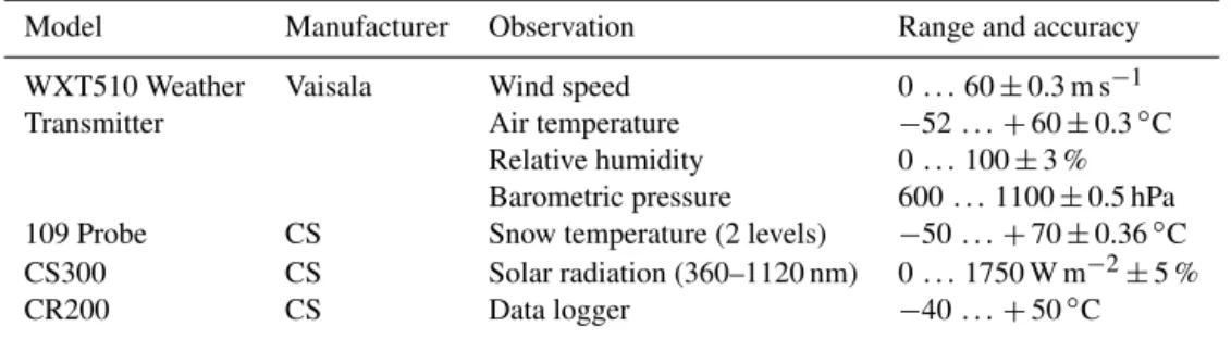
Table 1.Instruments and specifications used on the portable weather station deployed during the field surveys at the northern study sites.
Model Manufacturer Observation Range and accuracy
WXT510 Weather Vaisala Wind speed 0 . . . 60±0.3 m s−1
Transmitter Air temperature −52 . . .+60±0.3◦C
Relative humidity 0 . . . 100±3 %
Barometric pressure 600 . . . 1100±0.5 hPa
109 Probe CS Snow temperature (2 levels) −50 . . .+70±0.36◦C
CS300 CS Solar radiation (360–1120 nm) 0 . . . 1750 W m−2±5 %
CR200 CS Data logger −40 . . .+50◦C
made of insulation foam and Teflon-coated steel, able to hold a snow volume of 35×35×10 cm3.
The size of the trays selected for these experiments is as large as possible within the constraints of handling and weight. In this way, the snow contained is less affected by the small-scale eddies in the wind field caused by the discon-tinuity in the surface of the snow, which may play a appre-ciable role in the sublimation rate (Earman et al., 2006). The change of mass and the weight of meltwater in the lysime-ter were measured with a hand weighing scale Kern HDB (5K5) with a accuracy of 5 g, which for the 1260 cm2of the pan gives us a resolution of 0.04 mm of SWE. During the snowmelt period, the setting-up and loading of the pans with snow is done early in the morning, when the snow structure is more stable. The snow probe is previously cut and then loaded into the pan by a sliding movement to keep the snow surface and structure as undisturbed as possible. In order to facilitate this operation, one of the short sides of the top tray can be removed. The pans are positioned with the top surface of the loaded snow flush with the original snow surface sur-rounding the pan, but safely separated from it to avoid mass exchange. In order not to disturb the snow properties, mea-surements are separated as much as possible in time (2–5 h). Measurement accuracy is preferred over its timing, keeping in mind that the understanding of the processes requires the same time resolution as the process itself, which in the case of evaporation may be hourly or higher (Lundberg, 1993). Each test lasts no more than 24 h. On warm days with plenty of snowmelt, the test ends when the structure and surface of the snow samples begin to be unrepresentative of the sur-rounding snow.
Additionally, some snow properties required by the model were also measured during each field test. Albedo was mea-sured using a hand pyranometer, Solar Power ISM400 (400– 1100 nm), and snow density was estimated by gravimetric determinations of 1/3 L core samples obtained in situ. Fi-nally, the snow temperature was regularly measured during each test to establish the initial energy state of the snow and to check the correct performance of the snow model during the associated simulations.
3.3 Meteorological data during field surveys
During each snow ablation field test, extensive monitoring of the meteorological variables required by the model was performed by a complete weather station. The tests on the southern face of Sierra Nevada were carried out in an area within a radius of 20 m from the permanent weather station at the Refugio Poqueira monitoring site, at 2500 m a.s.l. On the northern face, the field tests were located at different points throughout the area above the town of Pradollano, at alti-tudes ranging from 2400 to 2600 m a.s.l., where a portable weather station was installed close to the ablameter device. In both cases, following the indications of Lundberg (1993), the ablameter was located upwind of the station to guaran-tee negligible disturbances of the meteorological conditions at the test point. Tables 1 and 2 show the main characteristics of the sensors installed in each weather station. At Refugio Poqueira, temperature,Ta, and relative humidity, RHa, were measured at 2.5 m above the snow surface, and wind speed at 3.0 m. At the portable weather stations, these heights change to 0.6 and 0.8 m respectively. The air vapour pressure was calculated fromTa and RHa using the empirical relation in Dingman (2002). Finally, solar radiation was measured using silicon photovoltaic pyranometers in both cases, while down-ward longwave radiation could be measured at the permanent station of Refugio Poqueira but not at the portable station at Pradollano. Both stations were managed by Campbell Scien-tific data loggers with a 1 s frequency of measurement and 1 to 5 min averaging record of the outputs.
4 Results
Table 2.Instruments and specifications used on the permanent weather station at the Refugio Poqueira monitoring point.
Model Manufacturer Observation Range and accuracy
HMP45C Vaisala Air temperature −40 . . .+60±0.3◦C
Relative humidity 0.8 . . . 100±3 %
RPT410F Druck Barometric pressure 600 . . . 1100±0.5 hPa
SP-Lite Kipp & Zonen Solar radiation (400–1100 nm) 0 . . . 1500 W m−2±5 %
CGR3 Kipp & Zonen Longwave radiation (4500–42 000 nm) −250 . . .+250 W m−2±5 %
05103-45 Alpine Young Wind vector 0 . . . 100±0.3 m s−1
CR10X CS Data logger −40 . . .+50◦C
T-200B w/Alter Shields Geonor Precipitation 0 . . . 600±0.1 mm
Table 3.Summary of the 15 data sets extracted from the 10 field campaigns with their date, duration, sky condition (N, night; S, sunny; O, overcast; C, cloudy), main weather drivers (wind speed,U; relative humidity, RHa; air temperature,Ta), measured evaposublimation (Eobs) and melting (Mobs) rates, measured snow albedo (α), and main topographic features of the test sites.
Test Date Duration Sky U RHa Ta Mobs Eobs α Slope Aspect S/N (h) condition (m s−1) (%) (◦C) (mm h−1) (mm h−1) (◦) face
1 12 Mar 2015 8.6 N 3.2 32 4.0 0.00 0.041 0.53 15 SW S
2 10 Apr 2014 4.6 S 2.1 34 10.5 4.18 0.044 0.62 23 SW N
3 27 Feb 2014 2.4 O 7.2 81 −1.0 0.00 0.041 0.8 3 W N
4 28 Jan 2014 5.2 S 4.3 46 −1.0 0.00 0.113 0.59 7 NW N
5 23 Jan 2014 4.3 S 8.4 70 −4.4 0.00 – 0.63 2 W N
6 28 Nov 2013 3.3 C 1.3 86 −3.4 0.00 0.020 0.75 20 N N
7 15 Mar 2013 5.0 S 1.3 49 3.2 1.51 – 0.62 5 S S
8a 1 Mar 2011 12.8 N 2.4 62 −9.3 0.00 0.000 0.8 8 S S
8b 2 Mar 2011 5.3 S 1.9 55 −7.7 0.00 −0.036 0.8 8 S S
8c 2 Mar 2011 2.6 S 1.6 63 −4.2 0.00 0.031 0.8 8 S S
9 29 Apr 2010 10.1 N 3.6 47 9.3 – 0.015 0.45 2 S S
10a 10 Mar 2009 11.8 N 5.6 15 3.9 0.00 0.111 0.67 12 S S
10b 11 Mar 2009 3.5 S 0.5 46 9.2 1.19 0.000 0.67 12 S S
10c 11 Mar 2009 13.8 N 2.6 37 4.9 0.00 0.047 0.67 12 S S
10d 12 Mar 2009 3.0 S 2.4 25 5.0 0.11 0.025 0.67 12 S S
4.1 Measurements of melt and evaposublimation
Table 3 summarises the main meteorological and snow mass fluxes measured for each of the 15 data sets obtained during the 10 field campaigns. The number of the field in the first column identifies the measurement campaign. Two of them (tests 8 and 10) are divided into three and four stationary periods each because of the observed change of the meteoro-logical forcing conditions (solar radiation, air or snow tem-perature, and even wind speed), mainly due to the transition from daytime to night-time. The date and duration of each data set are also recorded. The meteorological conditions over each test period are summarised as the average wind speed, relative humidity, temperature, and shortwave radi-ation state (sunny “S”, partially cloudy “C”, overcast “O”, or night “N”). The total melt and evaposublimation amounts measured with the ablameter are expressed in mm h−1. Fi-nally, information about albedo, α, and topography (slope, aspect, and face of Sierra Nevada, north or south) of the ex-act monitoring position is also shown.
The melting measurement relies on the correct drainage from the upper tray, which may sometimes be incomplete. We paid special attention to avoid the refreezing of meltwater in the drain holes, which was not observed in any of the per-formed tests. Three observations, one related toMin test 9 and two other related toEin tests 5 and 7, had to be rejected because they presented measurement errors due to accidents during the experimental work.
Figure 2.Photographs of the evaporation pan with lysimeter used in this study. In the sequence we can see(a)the load of the snow sam-ple by sliding of the upper tray,(b)handling of the complete device during weight, and(c)repositioning of the device to its measuring position.
snowpack required a mean air temperature above 9◦C for this to occur.
In contrast, evaposublimation is a continuous phe-nomenon, albeit at low rates. Only in two of the tests (8a and 10b) was there a complete absence of measured vapour flux; that is, there was no change of weight in the trays. The first of them (test 8a) is a night-time test over recent cold snow, at very low air temperature (−9.3◦C) and with
light wind (2.4 m s−1). These meteorological conditions are very similar to those encountered in the consecutive test 8b, which is the only one with a measured net deposition– condensation (gain of mass in the trays) and with an intense rate (0.036 mm h−1 during 5.3 h of test). Under the mete-orological conditions in test 8a, carried out from 18:35 to 04:00 CET, the expected behaviour is an initial sublimation while the snow cools from its “warmed” initial state to its night balanced state. Once the snow reaches its equilibrium temperature, the following deposition–condensation is the only mechanism to compensate longwave losses, which bal-anced in the end the initial loss of mass in the trays, as mea-sured. The other test without noticeableEis 10b, carried out on a sunny day with high air temperature (9◦C) and very low wind speed (0.5 m s−1), the lowest measured speed. These data may indicate that there is a threshold of wind that can inhibit the vapour fluxes; otherwise, these fluxes are always present. Even though their maximum rates were 1 order of magnitude under those for melting, accumulation of evapo-sublimation throughout the year may result in an substantial total amount in the annual mass budget. Vapour loss rates above 0.04 mm h−1 were measured equally on days under intense melting (test 2) and on cold wet days (test 3). Maxi-mum evaposublimation rates of 0.11 mm h−1were measured under favourable weather conditions for evaposublimation
(cold days with low relative humidity and gentle wind speeds around 5.0 m s−1).
4.2 Measurements vs. model estimates – test periods Table 4 shows the results obtained when the energy balance snow model is applied over the test periods. The differences between measured and simulated melting/evaposublimation rates are also presented for each test as statistics for the error of the simulation.Esim only refers to the positive outgoing flux. WhenEis simulated with a negative sign, it is taken as deposition–condensationCsim. The last column showsz0, which was estimated for each test by minimising the sum of the mean errors (ME) ofE andM. The comparison of measured and simulated values ofE andM are plotted in Fig. 3. The goodness of the calibration is determined by using the ME, the mean absolute error (MAE), and the root mean square error (RMSE). The agreement between model and ob-servations for bothEandMis very high, except for one out-lier, which is circled. RMSE forEis 0.008 mm h−1(6.7 % of the maximumEmeasured), while forMit is 0.009 mm h−1 (0.6 % of the maximumM).
The selected values forz0(Table 4) mostly range from 1.0 to 0.3 mm. These values are lower than the calibrated value in Herrero et al. (2009), 2.5 mm. Test 3 is the only one with a lower value, 0.1 mm, and it corresponds to conditions that promoted the formation of a thin layer of ice on top of the snow, so its surface appeared particularly smooth. In gen-eral,z0under 0.5 mm is only estimated on the northern face of Sierra Nevada in tests performed in January or February. In this area at that time, snow is more likely to form sur-face ice layers with a noticeable influence onz0. The aver-age value ofz0for all these field campaigns is 0.61 mm. The second calibration parameter of the model,KH0, was found to perform adequately throughout all the cases if taken con-stant and equal to 1 W m−2K−1, which is in agreement with other studies (Jordan, 1991; Jordan et al., 1999), and lower than the previously obtained value of 6 W m−2K−1 in Her-rero et al. (2009). The inclusion of a decaying albedo instead of a constant value, together with the more accurate value of the longwave term in the energy balance equation, is one of the reasons behind these differences, together with the use of water fluxes as optimisation objectives instead of snow depth values. In the next section we test the model performance for snow depth under these calibrated values.
Table 4.Summary of the simulated (sim) results (M, melting;E, evaposublimation;C, deposition–condensation) from the energy balance model for each data set period, together with the simulated energy flux terms (shortwave radiation,K; longwave radiation,L; sensible-heat exchange,H; latent-heat exchange, LE) and the calibrated values for the model parameters (roughness length,z0; constant sensible-heat transfer coefficient in windless conditions,KH0=1 W m−2K−1).
Test Msim Esim Csim(-Esim) ErrorM ErrorE Ksim Lsim Hsim LEsim z0 (mm h−1) (mm h−1) (mm h−1) (mm h−1) (mm h−1) (W m−2) (W m−2) (W m−2) (W m−2) (mm)
1 0.00 0.041 – 0.00 0.000 0.0 −75.0 108.3 −27.8 0.9
2 4.17 0.046 – −0.01 0.002 380.6 −61.1 102.8 −30.6 0.5
3 0.00 0.049 – 0.00 0.008 72.2 −44.4 11.1 −33.3 0.1
4 0.00 0.112 – 0.00 0.002 166.7 −91.7 16.7 −77.8 0.3
5 0.00 0.131 – 0.00 – 197.2 −97.2 −11.1 −88.9 0.3
6 0.00 0.010 0.000 0.00 −11 22.2 −11.1 16.7 −5.6 1.0
7 1.52 0.042 – 0.01 – 316.7 −166.7 22.2 −27.8 0.8
8a 0.00 0.002 0.002 0.00 0.000 0.0 −75.0 52.8 0.00 0.5
8b 0.00 0.004 0.003 0.00 0.037 102.8 −100.0 38.9 −2.8 0.5
8c 0.00 0.029 – 0.00 −0.002 158.3 −88.9 −11.1 −19.4 0.5
9 0.75 0.019 0.002 – 0.000 2.8 −38.9 119.4 −13.9 1.0
10a 0.00 0.130 – 0.00 0.019 5.6 −88.9 172.2 −88.9 0.7
10b 1.20 0.003 – 0.01 0.003 227.8 −138.9 22.2 −2.8 0.7
10c 0.00 0.041 – 0.00 −0.006 2.8 −69.4 83.3 −27.8 0.7
10d 0.14 0.042 – 0.03 0.017 127.8 −94.4 72.2 −27.8 0.7
Night test 8a, with 0 mm of measuredE, is simulated by the model as a mixed state with an initial loss and a subse-quent gain of vapour, reaching a balance by the end of the test. This is consistent with the hypothesis made in the pre-vious section, even though the balance point is reached by simulating a deposition–condensation rate much lower than that measured in the following hours, during test 8b. This test 8b stands out as an outlier because a high deposition– condensation rate (negative E) of −0.036 mm h−1 is
mea-sured (circled in Fig. 3a) from 07:20 to 12:40 CET, but it is simulated as only −0.004 mm h−1 during the night
inter-val. According to the model, this deposition–condensation occurs from 04:00 CET to dawn, with a low air temperature (−7.7◦C), not too high relative humidity (55 %), and light
wind (1.9 m s−1) over very cold snow (−17.5◦C). Once the sun rises, the model predicts sublimation as the snow tem-perature increases to balance with the air temtem-perature. This difference in the deposition–condensation rate is not likely to be due to a measurement error but to a modelling issue. The model succeeded in reproducing the sequence of deposition– condensation and sublimation but missed the deposition– condensation rate by an order of magnitude. Further work is needed to test this deviation by the model and identify its sources.
To estimate the sensitivity of the model to changes in z0 within the ranges found in the field, we repeated the prior simulations considering a constantz0value equal to its aver-age calibrated value. The results are plotted in Fig. 4. The error made when simulating with z0=0.61 mm increases
slightly inE(ME increases from 0.002 to 0.003 mm h−1and RMSE from 0.008 to 0.012 mm h−1). The increase in the
er-Figure 3.Measurements versus model estimates of evaposublima-tion (E) and melting (M) for the different test periods using the cal-ibrated values for each test in Table 4. Each plot includes the root mean square error (RMSE), the mean error (ME), and the mean ab-solute error (MAE). The line indicates a 1 : 1 relationship between observed (obs) and simulated values (sim).
rors inM(ME from 0.003 to 0.051 mm h−1and RMSE from 0.009 to 0.164 mm h−1) is concentrated in one particular test that moves away from the 1 : 1 line, though errors still remain small as ME is only 3.4 % of the maximum measuredM. It appears that the range of variation in measurements ofz0is low enough not to affect the results substantially.
4.3 Annual simulation
Figure 4.Measurements versus model estimates of evaposublima-tion (E) and melting (M) for the different test periods using a con-stantz0of 0.61 mm. Each plot includes the root mean square error (RMSE), the mean error (ME), and the mean absolute error (MAE). The line indicates a 1 : 1 relationship between observed (obs) and simulated values (sim).
test periods. Thus,KH0andz0are supposed fixed and equal to 1 W m−2K−1and 0.61 mm respectively.
The validation of the snow model was assessed in terms of the snow depth observed at the Refugio Poqueira station. Figure 5a shows how the model reproduced the main patterns in the intra- and interannual cycles in the snowpack. The cor-rect simulation of accumulation and melting over time and the good match of the timing of the different intra-annual melting cycles means that the model is computing adequately not only the snow depth and SWE time series but also the cumulative energy balance of the snowpack (López-Moreno et al., 2013). Figure 5b and c show the observed and sim-ulated annual maximum accumulation and duration of the snowpack respectively. In both cases the simulated values fit well with the observations regardless of the wet–dry charac-ter of the year and the number of snowmelt cycles encoun-tered. For the period 2009/2010–2012/2013, the maximum snowpack depths measured ranged from 627 to 1400 mm, while the number of cycles with total disappearance of the snow varied between three and seven. In general, autumn and spring precipitation events fall as snow but melt within a few days. However, there are drier or warmer years when complete melt is reached even during the winter. Snowpack duration ranged from 85 to 138 days. In the simulation, the ME and the RMSE were −81 and 235 mm for daily snow
depth, 63 and 136 mm for annual maximum depth, and 2.8 and 10.5 days for annual snowpack duration.
Figure 6 shows the course of simulated cumulative snow-fall, SWE, evaposublimation, and snowmelt for each of the 7 hydrological years under study. The average annual ratio of total evaposublimation versus total ablation is 30.6 %, oscil-lating from a minimum of 24.2 % in 2010/2011 to a maxi-mum of 32.8 % in 2014/2015. The year with the highest total vapour loss is 2009/2010, with 204 mm, while the year with the lowest loss is 2011/2012 with 94 mm. Despite this low value, the percentage of evaposublimated snowfall is high for this year, 29.4 %. In general, years with low total snowfall
re-Figure 5. (a)Snow depth in millimetres simulated for each snow season at the Refugio Poqueira site from the hydrological year 2008/2009 to 2014/2015. The grey crosses show the observed snow depth for years 2009/2010 to 2012/2013.(b)Observed (obs) ver-sus simulated (sim) annual maximum snow depth in millimetres at this site.(c)Observed versus simulated annual duration of the snow depth in days at this site. The line at(b)and(c)indicates a 1 : 1 rela-tionship between observed and simulated values. Each plot includes the root mean square error (RMSE), the mean error (ME), and the mean absolute error (MAE).
Figure 6.Cumulative snowfall together with the stacked cumula-tive snowmelt (M) and cumulative evaposublimation (E) (in mm) for each snow season at the Refugio Poqueira site from the hydro-logical year 2008/2009 to 2014/2015. The white area between the snowfall and the stackedMandErepresents the instant snow water equivalent (SWE) during the year. The percentage at the end of ev-ery season indicates the ratio of annual evaposublimation compared to total ablation.
sult in a higher percentage of evaposublimation and a higher number of melting cycles. The model also estimates a mean annual deposition–condensation of 0.9 % of the total snow-fall (4.8 mm yr−1).
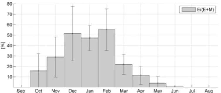
max-Figure 7.Mean monthly ratio of evaposublimation compared to to-tal ablation during the year at the Refugio Poqueira site for the study period 2008–2015. Whiskers represent standard deviation from the mean.
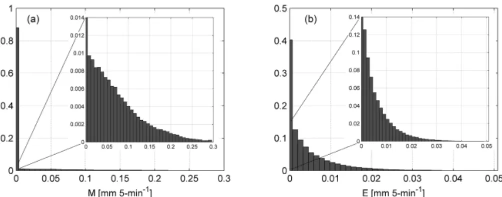
imum rates for M are approximately 1 order of magnitude higher than the rates forE, althoughMis 0 or very close to 0 for almost 90 % of the time with snow cover, compared to the 40 % associated with zero values ofE.
Figure 7 represents the ratio of the evaposublimation ver-sus total ablation in each month of the year, averaged over the entire simulated period. The graph highlights the seasonal variations of the percentage of evaposublimation on an an-nual basis. In the months of December, January, and Febru-ary, evaposublimation accounts on average for 47–51 % of all the ablation that takes place. Snowmelt is present in these winter months, but with a moderate intensity (Fig. 9). During the following months, the evaposublimation ratio decreases sharply as snowmelt dominates, decreasing to approximately 22 % in March, 12 % in April and 4 % in May. MonthlyM always dominates when compared toE(Fig. 9), increasingly during the spring months. However, the standard deviation of M is always higher than that of E, and it has the same order of magnitude as the mean itself, which means that zero melt can be expected in every month but January, March, and April. In contrast, monthlyEis less variable and shows lower standard deviations.
The cumulative annual energy fluxes in W m−2 for the period 2008/2009–2014/2015, together with their mean and standard deviation proportion, are shown in Fig. 10. Warm-ing fluxes (sensible heat exchange, H, and shortwave radi-ation,K) are on the positive side of the xaxis while
cool-ing fluxes (advected heat associated with precipitation,UR,
latent-heat exchange, LE, and longwave radiation,L) appear on the negative side. Their average fractions of the energy balance are 60 % for H and 40 % forKas positive (warm-ing) fluxes, and−54 % forL,−32 % for LE, and−14 % for
URas negative (cooling) fluxes. The standard deviations are small compared to those from the mass fluxes,L being the most variable flux with 7 %. Even though L dominates on average over LE as a negative flux, there is one particular year (2010/2011) in which both fluxes are equal. The ratio betweenHandKalso changes moderately between years.
5 Discussion
The turbulent heat transfer terms are probably the most un-certain contribution to solving the energy budget over the snow. Flux-profile and bulk transfer approaches have been shown to be problematic over sloping terrain to determine turbulent fluxes (Hock, 2005). In general, snow in mountain-ous areas must always be considered as a non-uniform sur-face, either because of the presence of patchy snow, obstacles such as rocks or shrubs that stand out of the snow surface on shallow snowpacks, or topographic gradients themselves. Besides the usual wind exposure of higher elevations, gravity winds usually develop even during calm days, promoting tur-bulent transfer under every meteorological condition (Feick et al., 2007). These turbulent terms include the calibration pa-rameters used in the energy balance modelling, one referring toH (KH0) and the other to bothHand LE (z0). The deter-mination of both parameters, together with the consideration of stability effects, are the major challenges of the physically based snow models. These calibration parameters appear to be very site dependent, according to the wide spectrum of variation described in the literature. In this work, these co-efficients have been calibrated for Sierra Nevada (Spain) at approximately 2500 m a.s.l. using detailed measurements of mass fluxesEandM, with a final result of 1 W m−2K−1for KH0and 0.61 mm forz0as a seasonal average value. Despite the large uncertainty that still exists regarding the roughness length of the different types of snow surfaces (Martin and Lejeune, 1998), the measurements for this study area sug-gest a range ofz0from 0.1 mm, for very smooth icy surfaces, to 1.0 mm on metamorphosed snow that shows surface forms as snow cups.
Figure 8.Probability density function of the mean snowmelt (M) and evaposublimation (E) rates in mm 5 min−1at the Refugio Poqueira site
from the hydrological year 2008/2009 to 2014/2015. The zoom on each plot shows the distribution without the influence of the zero-values.
Figure 9.Mean monthly snowmelt (M) and evaposublimation (E) rates in mm month−1during the year at Refugio Poqueira site for
the study period 2008–2015. Whiskers represent standard deviation from the mean.
Figure 10.Annual mean energy balance (W m−2) over the snow-pack at the Refugio Poqueira site from the hydrological year 2008/2009 to 2014/2015 and average proportions of the fluxes, warming as positive (exchange of sensible heat,H, and shortwave radiation,K) and cooling as negative (heat advected to precipita-tion,UR, exchange of latent heat, LE, and longwave radiation,L).
the process as long as it remains below 80 %, a value that indicates its supporting role to the wind effects.
Our evaposublimation rates are somewhat higher than those measured by Kaser (1982), who found maximum sub-limation rates of 2 mm d−1 in the Alps during the sum-mer at 3000 m a.s.l., somehow balanced with a
correspond-ingly high deposition–condensation overnight. However, in a high latitude area like Canada, Valeo et al. (2005) recorded maximum values of sublimation equal to 6.3 mm in 8 h (0.8 mm h−1 on average) in Alberta (51◦N), while Jack-son and Prowse (2009) simulated mean vapour loss of 0.4 mm d−1 in open sites at Okanagan Basin (49◦N) with SNTHERM (Jordan, 1991). The latter also simulated max-imum melting rates of 40.5 mm d−1, similar to the values found in this study. Even at this latitude, events of warm and dry air masses can occur during winter (the Chinook, popularly translated as “snow-eater”, is an example of foehn winds), which occasionally enhance sublimation losses from the snow up to these values. In warmer areas, conditions to record high sublimation losses are easier to find. Avery et al. (1992) measured a maximum evaposublimation loss of 8.5 mm d−1 under clear, dry, and windy conditions on the Colorado Plateau of Arizona at 35◦N and 2100 m a.s.l. In any case, modelled or simulated, it is reported than this rate is highly variable depending on the local conditions of the wind regime (Feick et al., 2007), on the meteorology and, therefore, on the time of the year when the snowpack accu-mulates.
During our field measurements, one of the tests in Refugio Poqueira showed a strong deposition–condensation rate of 0.036 mm h−1 that could not be simulated with the model. The simulation of hoar growth in complex terrain is a difficult task since it demands data of the local wind regime with a spatial resolution under 10 m (Feick et al., 2007), which was not accomplished for the tests in Poqueira, located 10 to 20 m away from the station. Further measurements and study are necessary to establish whether this deposition–condensation rate is a common phenomenon in the area, where problems with hoar and ice over structures (for example, at ski resorts) are often reported.
using physical models in approaching these processes. The difference in the annual evaposublimation between different climatic zones is related to the availability of those meteoro-logical states that favour evaposublimation. In Sierra Nevada, evaposublimation is present almost continuously to a greater or lesser extent, so its contribution becomes important on an annual basis. The worst-case scenario for high evapo-sublimation rates takes place when the snow pack accumu-lates early in the season (Avery et al., 1992). The impor-tance and variability of evaposublimation in Sierra Nevada agrees with other studies in warm and semiarid mountainous regions around the world, such as California (20 %, Marks and Dozier, 1992; 36 %, Leydecker and Melack, 2000), Col-orado (15 %, Hood et al., 1999; 17–43 %, Froyland, 2013), Canada (40 %, Gray and Prowse, 1993), the Andean Alti-plano (30–90 %, Vuille, 1996), the Atlas mountains (44 %, Schulz and de Jong, 2004; 7–20 %, Boudhar et al., 2016), and Israel (46–82 %, Sade et al., 2014), although its exact proportion depends greatly on the exact location of the sam-pling point and its altitude. At the Refugio Poqueira study site (2500 m a.s.l., 37◦N), and in most of Sierra Nevada in general, year-to-year climate variability in precipitation and temperature interacts non-linearly to allow the development of a highly heterogeneous snowpack, which leads to the cor-responding variability in the percentage contribution of evap-osublimation to total snow ablation.
6 Conclusions
In this study we have quantified the evaposublimation rates and the rest of the energy balance terms of the seasonal snow-pack in the semiarid region of Sierra Nevada (37◦N). The 15 field data sets performed succeeded in validating the phys-ically based snow model designed by Herrero et al. (2009). Although the measurement based on manually weighed trays is a traditional and not automated method, it achieves high accuracy thanks to the technical characteristics of the cur-rent weight measuring instruments. The measurements have confirmed the constant presence of evaposublimation from the snow in this semiarid environment, detecting maximum rates of 0.11 mm h−1in periods that were neither particularly dry nor particularly windy. Melting snow on warm days can reach much higher rates, up to 4.18 mm d−1, but its effect takes place in shorter periods than those affected by evap-osublimation, which is more persistent for different meteo-rological conditions. Throughout the period when the snow is accumulated on the soil surface, evaposublimation occurs during 60 % of the time, while snowmelt only occurs dur-ing 10 %. With these data, the energy-balance snow model was calibrated using two main parameters, both associated with turbulent fluxes: the roughness length of the snow z0 and the sensible-heat transfer coefficient in windless condi-tionsKH0.KH0was set to 1 W m−2K−1, whilez0was found to range between 0.1 mm over recent snow with an icy
sur-face and 1.0 mm over mature snow with big grain size and an irregular surface. The mean value forz0was 0.61 mm.
The model satisfactorily reproduced the evaposublima-tion and melting rates during the monitored periods. Situa-tions with simultaneous melting and evaporation were also correctly simulated. From these results, the continuous per-formance of the model at the Refugio Poqueira monitor-ing site (at 2500 m a.s.l.) durmonitor-ing the 2008–2015 period, pro-duced an estimated evaposublimation value between 94 and 204 mm yr−1, from a total snowfall of 320 to 676 mm yr−1, which accounts for between 24 and 33 % of the total annual accumulated snow. On a daily basis, the evaposublimation rate reached a mean value of 1.2 mm d−1, with a maximum of 7.2 mm d−1with hourly peaks of 0.49 mm h−1being sim-ulated on very windy days.
Regarding the energy balance, we were able to estimate that 32 % of the cooling energy is due to the latent-heat trans-fer term, which is considerable. Wind is the key element that establishes the final weight of this term in the energy bud-get for every season. Due to its proximity to the sea, and its high altitude compared to the neighbouring mountains, Sierra Nevada is a wind-exposed mountain range, which ex-plains the relevant influence of this term on the snow regime over the mountain range.
The annual energy and mass balance over the snowpack is sensitive to small changes in variables governing the weather regime and/or their timing. Due to the elevational gradients and the seasonal and annual climate variability, high variabil-ity of the weather drivers can usually be found both spatially and over time in semiarid high mountain environments. Since simultaneous and intense monitoring of the snowpack is not feasible over these areas, the availability of a reliable snow model to infer the distribution of evaposublimation through-out Sierra Nevada and to further simulate the evolution of the snowpack is an important and useful tool. In these regions, the impact of this return of water to the atmosphere is appre-ciable on the hydrology and on the availability of water as a resource. The results shown in this study are a first and es-sential step for estimating the influence of snow dynamics on runoff and water storage in the area and for assessing water planning in the short and medium term. The implications for adaptation strategies are also relevant in a scenario of change in the energy budget regime.
7 Data availability
Appendix A: Snow mass and energy balance equations The instantaneous mass and energy balance in the one-layer control volume per unit of surface area is described as fol-lows:
dm
dt =R−E+W−M, (A1)
d(m·u)
dt =K+L+H+G+R·uR−E·uE
+W·uW−M·uM, (A2)
where m denotes the water mass in the snow column (SWE), and u is the internal energy per unit of mass (U for total internal energy). Regarding mass fluxes, R de-notes the precipitation,E represents water vapour diffusion (evaposublimation–deposition–condensation),Wis the mass transport due to wind, andMis the melting water. The energy fluxes are the solar or shortwave radiationK, the thermal or longwave radiationL, the exchange of sensible heat with the atmosphere H, the heat exchange with the soil G, and the advective heat terms associated with each of the mass fluxes (uR,uE,uW, anduM) which refer to the unitary internal
en-ergy of each of the mass fluxes considered.
Equations (A1) and (A2) form a coupled set of first-order, non-linear ordinary differential equations. They are solved with a first-order finite difference approximation with a 5 min step time and an iterative algorithm (Herrero et al., 2009) that can reduce the time step in situations of numerical instability. Precipitation, directly measured by the weather station in every case, is partitioned into rain or snow using the wet bulb temperature, Tw. This is taken as the temperature for the rain, which is considered frozen ifTw≤0◦C.Twcan be estimated from the temperature of the air,Ta, the relative hu-midity of the air,Wa, and the atmospheric pressure,Pa, using Normand’s rule (e.g. Stull, 2000).
The shortwave albedo of the snow,α, is a property of the snowpack surface that changes with time, usually decreasing as the snow grain size increases. In this model, if no measure-ments are available,αis parameterised as a function of the snow surface age between a maximum value of 0.8 for recent snow and a minimum of 0.4 for old snow. The ageing process is predicted with a linear decay with time (Baker et al., 1990; Pimentel et al., 2013), slower for cold snow (0.006 day−1) than for melting snow (0.018 day−1). New snowfall refreshes αat a rate of 0.05 mm−1of new SWE.
The equivalent atmospheric emissivity,εa, is used to cal-culate the incoming longwave radiation,Ldown, from the at-mosphere. The model can work with direct measurements of Ldown where available or estimateεa from the near-surface temperature, relative humidity, and clearness index (related to solar radiation and cloudiness) using the empirical expres-sion of Herrero and Polo (2012).
The turbulent energy diffusion terms for water vapour LE as well as for sensible heatH can be resolved by basing cal-culations on the physics of turbulent transfer near the ground, as explained, for example, in Dingman (2002):
LE=E·u E= KLE
8M8V
va(esn−ea), (A3)
H=
K
H 8M8H
va+KH0
(Ta−Tsn), (A4) whereKLE is the bulk latent-heat transfer coefficient,KH is the bulk sensible-heat transfer coefficient, KH0 is the sensible-heat transfer coefficient in windless conditions,vais the wind speed at the reference altitude,eais the air vapour pressure at the reference altitude,esnis the saturation vapour pressure for the snow temperature (Tsn)Tais the air temper-ature at the reference altitude and8M,8V, and8H are the
stability-correction factors for momentum, water vapour, and sensible heat for non-adiabatic temperature gradients, intro-duced to account for the buoyancy effects that may enhance or dampen the turbulent transfers because of the tempera-ture gradient over the surface. There are numerous empirical expressions for these correction coefficients, depending on the Richardson number or the Monin–Obukhov length (Price and Dunne, 1976; Anderson, 1976; Oke, 1987; Cline, 1997; Jordan et al., 1999). However, application to actual wind and temperature conditions may lead to values of these coeffi-cients that fall outside the limits for which they were em-pirically defined. This fact, as well as the uncertain improve-ment in the accuracy of the results with their application (e.g. Hock, 2005), has led certain authors to reject them com-pletely (Tarboton and Luce, 1996; Herrero et al., 2009), or limit their use to smaller ranges (Koivusalo and Kokkonen, 2002).
KLEandKHare defined as follows:
KLE=uE0.622ρa Pa
k2 h
lnza−zd z0
i2, (A5)
KH=ρaca k 2
h
lnza−zd z0
i2, (A6)
where ρa is the mass density of air in kg m−3, ca is the heat capacity of air (at constant pressure, 0.001005 MJ kg−1K−1), P
the gas constant for airRa(0.288 for the units given),ρacan be calculated as follows:
ρa= Pa
TaRa. (A7)
The KLE term includes the unitary internal energy uE ad-vected toE, and it appears in Eq. (A2). Ifesn> ea, evapora-tion occurs anduE is the advected heat of the water vapour that moves out from the surface layer into the air above mea-sured. The internal energy of this flux as it moves out of the snow into the atmosphere will be that of water vapour with the temperature of the surfaceTsnwith respect to the selected reference state. Therefore, the calculation ofuEis indifferent to the initial state of water on the surface of the snow and is the same for sublimation (with frozen surface) and evapora-tion.
uE=λv+cevTsn,ifesn> ea, (A8a) uE=cevTa,ifesn< ea, (A8b) where λv is the latent heat of vaporisation (2.47 MJ kg−1) and cev is the heat capacity of water vapour (0.001850 MJ kg−1K−1 at standard conditions STP). If esn< ea, then water vapour molecules enter the surface at Ta, where they condense. Their unitary internal energy will be that of Eq. (A8b).
The snow densityρsnis mainly needed in the model for the calculation of the snow depthhsn. It is considered uniform in the snowpack, and its evolution is calculated from an ini-tial value for new snowρsn-minthat is gradually modified in time through percolation, refreezing (both due to meltwater and rain), deposition–condensation, and new snowfall. There are two kinds of maximum density: one,ρsn-max, is due to grain growth associated with percolation; the other,ρsn-frz, is a possible maximum density reached through internal re-freezing of water. Density increase due to percolation is rep-resented by a parameterisation that makes use of melting rate M, a growth coefficientk1ρwith units of kg L−1mm−1, and
a normalised density2sn:
1ρsn=M·k1ρ·2sn(ρsn), (A9) 2sn= ρsn−ρsn-min
ρsn-frz−ρsn-min, (A10)
with ρsn-min=0.1 kg L−1, ρsn-max=0.5 kg L−1, ρsn-frz=
0.65 kg L−1, andk
1ρ=0.008 kg L−1mm−1ifρsn< ρsn-max,
Acknowledgements. We are grateful to Sergio Torres, Agustín
Millares, Zacarías Gulliver, Marta Egüen, and Rafael Pimentel for their help in the field work. This study was funded by the Spanish Ministry of Economy and Competitiveness – MINECO (project CGL2011-25632, “Snow dynamics in Mediterranean regions and its modelling at different scales. Implications for water resource management”, and project CGL2014-58508R, “Global monitoring system for snow areas in Mediterranean regions: trends analysis and implications for water resource management in Sierra Nevada”). We thank Werner Eugster and one anony-mous reviewer whose comments helped to improve this manuscript.
Edited by: M. Schneebeli
Reviewed by: W. Eugster and one anonymous referee
References
Alter, J. C.: Shielded storage precipitation gages, Mon. Weather Rev., 65, 262–265, 1937.
Anderson, E. A.: Development and testing of snow pack energy bal-ance equations, Water Resour. Res., 4, 19–37, 1968.
Anderson, E. A.: A point of energy and mass balance model of snow cover, Tech. Rep. NWS 19, NOAA, Department of Commerce, 1976.
Andreas, E. L.: A relationship between the aerodynamic and phys-ical roughness of winter sea ice, Q. J. Roy. Meteor. Soc., 137, 1581–1588, 2011.
Avery, C. C., Dexter, L. R., Wier, R. R., Delinger, W. G., Tecle, A., and Becker, R. J.: Where has all the snow gone? Snowpack sub-limation in northern Arizona, in: Proceedings of the 60th West-ern Snow Conference, 84–94, Colorado State University, Jackson Hole, WY, 1992.
Baker, D., Ruschy, D., and Wall, D.: The albedo decay of prairie snows, J. Appl. Meteorol., 29, 179–187, 1990.
Baldocchi, D. D., Hincks, B. B., and Meyers, T. P.: Measuring biosphere-atmosphere exchanges of biologically related gases with micrometeorological methods, Ecology, 69, 1331–1340, 1988.
Barry, R. G.: Mountain weather and climate, Psychology Press, Routledge, Boca Raton, Florida, 2nd edn., 1992.
Bengtsson, L.: Evaporation from a Snow Cover – Review and Dis-cussion of Measurements, Nord. Hydrol., 11, 221–234, 1980. Boudhar, A., Boulet, G., Hanich, L., Sicart, J. E., and Chehbouni,
A.: Energy fluxes and melt rate of a seasonal snow cover in the Moroccan High Atlas, Hydrolog Sci. J., 61, 931–943, 2016. Braithwaite, R.: Aerodynamics stability and turbulent sensible-heat
flux over a melting ice surface, the Greenland ice sheet, J. Glaciol., 41, 562–571, 1995.
Brun, E., Yang, Z., Essery, R., and Cohen, J.: Snow-cover pa-rameterization and modeling, in: Snow and climate: physical processes, surface energy exchange and modeling, edited by: Armstrong, R. L. and Brun, E., 125–180, Cambridge University Press, 2008.
Calanca, P.: A note on the roughness length for temperature over melting snow and ice, Q. J. Roy. Meteor. Soc., 127, 255–260, 2001.
Cline, D., Elder, K., and Bales, R.: Scale effects in a distributed snow water equivalence and snowmelt model for mountain basins, Hydrol. Process., 12, 1527–1536, 1998.
Cline, D. W.: Snow surface energy exchanges and snowmelt at a continental, midlatitude Alpine site, Water Resour. Res., 33, 689–701, 1997.
Colbeck, S.: An overview of seasonal snow metamorphism, Rev. Geophys., 20, 45–61, 1982.
Datt, P., Srivastava, P., Sood, G., and Satyawali, P.: Estimation of equivalent permeability of snowpack using a snowmelt lysimeter at Patsio, northwest Himalaya, Ann. Glaciol., 51, 195–199, 2010. Dingman, S.: Physical hydrology, Prentice Hall, Upper Addle River,
New Jersey, 2nd edn., 646 pp., 2002.
Dionisio, M. Á., Alcaraz-Segura, D., and Cabello, J.: Satellite-based monitoring of ecosystem functioning in protected areas: recent trends in the oak forests (quer-cus pyrenaica willd.) of Sierra Nevada (Spain), in: Inter-national Perspectives on Global Environmental Change, edited by: Young, S. S. and Silvern, S. E., 355–374, InTech, available at: http://www.intechopen.com/books/ international-perspectives-on-global-environmental-change (last access: 3 December 2016), 2012.
Doty, R. D. and Johnston, R. S.: Comparison of gravimetric mea-surements and mass transfer computations of snow evaporation beneath selected vegetation canopies, in: Proceedings of the 37th Western Snow Conference, 57–62, Salt Lake City, UT, 1969. Earman, S., Campbell, A. R., Phillips, F. M., and Newman, B. D.:
Isotopic exchange between snow and atmospheric water vapor: Estimation of the snowmelt component of groundwater recharge in the southwestern United States, J. Geophys. Res.-Atmos., 111, D09302, doi:10.1029/2005JD006470, 2006.
Essery, R., Li, L., and Pomeroy, J.: A distributed model of blow-ing snow over complex terrain, Hydrol. Process., 13, 2423–2438, 1999.
Eugster, W. and Merbold, L.: Eddy covariance for quantifying trace gas fluxes from soils, SOIL, 1, 187–205, doi:10.5194/soil-1-187-2015, 2015.
Fassnacht, S.: Estimating Alter-shielded gauge snowfall undercatch, snowpack sublimation, and blowing snow transport at six sites in the coterminous USA, Hydrol. Process., 18, 3481–3492, 2004. Feick, S., Kronholm, K., and Schweizer, J.: Field observations on
spatial variability of surface hoar at the basin scale, J. Geophys. Res.-Earth, 112, F02002, doi:10.1029/2006JF000587, 2007. Föhn, P.: Short-term snow melt and ablation derived from heat-and
mass-balance measurements, J. Glaciol., 12, 275–289, 1973. Froyland, H. K.: Snow loss on the San Francisco peaks: Effects of
an elevation gradient on evapo-sublimation, Ph.D. thesis, North-ern Arizona University, 2013.
Froyland, H. K., Untersteiner, N., Town, M. S., and Warren, S. G.: Evaporation from Arctic sea ice in summer during the Interna-tional Geophysical Year, 1957–1958, J. Geophys. Res.-Atmos., 115, D15104, doi:10.1029/2009JD012769, 2010.
Garstka, W.: Snow and snow survey, in: Handbook of Applied Hy-drology, edited by: Chow, V., 10.10–10.12, McGraw-Hill, New York, 1964.