Welfare and growth effects of alternative fiscal rules for infrastructure investment in Brazil

(1)

No ₆₀₄ _{ISSN 0104-8910}

Welfare and Growth Effects of Alternative

Fiscal Rules for Infrastructure Investment in

Brazil

(2)

Os artigos publicados são de inteira responsabilidade de seus autores. As opiniões

neles emitidas não exprimem, necessariamente, o ponto de vista da Fundação

(3)

Welfare and Growth E¤ects of Alternative Fiscal

Rules for Infrastructure Investment in Brazil

Pedro Cavalcanti Ferreira

Graduate School of Economics - EPGE

Fundação Getulio Vargas

Leandro Gonçalves do Nascimento

Graduate School of Economics - EPGE

Fundação Getulio Vargas

May 20, 2005

Abstract

Key Words: infrastructure; public goods; welfare and growth; public debt.

(4)

1 Introduction

The productive impact of infrastructure has been investigated in the last years by

an increasing number of studies, starting with Aschauer’s (1989) pioneering article.

These studies use di¤erent econometric techniques and data samples to estimate

the output and productivity elasticity to public capital. Although the magnitudes

found vary considerably, the overall estimates (e.g. Aschauer (1989), Ai and

Cas-sou (1995), Easterly and Rebelo (1993) and Calderón and Servén (2003)) tend to

con…rm the hypothesis that infrastructure capital positively a¤ects productivity

and output.

At the same time, public investment in Brazil, as a share of gross domestic

product (GDP), has been falling for the last twenty-…ve years. From 1960 to 1980

public investment ratio averaged 4:0% of GDP, but it was only 2:2% in 2002.

Moreover, the decrease in infrastructure expenditure a¤ected virtually all sectors.

For instance, direct investment in roads from 1990 to 1995 was only, in real terms,

one …fth of those made in the 1970-1975 period (Ferreira and Maliagros (1998)),

while total public investment in the transportation sector today is less than 0:1%

of GDP. The reduction in relative public capital formation coincides with the

slowdown of GDP growth rates. While GDP per capita grew at around 3% from

1950 to 1980, in the following period this rate fell to less than 1%.

In this article we study the welfare and macroeconomic impact of government

actions when its productive role is taken into account. In this sense, we construct

and simulate a competitive general equilibrium model in which public investment

can be …nanced through a variety of sources. Our model basically starts from the

(5)

al-though the latter use an overlapping-generations framework, and add a budgetary

regime analogous to the general case presented in Greiner and Semmler (2000).

The model economy was solved by simulation techniques and parameters and

func-tional forms were calibrated to match features of the actual Brazilian economy.

Hence, the main motivation for this article is the interplay between …scal rules,

investment and growth. The paper’s core is whether (1) it would make sense to

raise public investment and (2) if so, under which …scal rule it is best to do it –

whether through tax …nancing, debt …nancing, or a cut in public consumption.

With respect to the …rst question, we …nd that even using very conservative

calibration for the elasticity of output to public capital, results show that, if the

public investment ratio returned to its before-1980 level, output growth would

be sizeable. Such result is robust to functional forms, reasonable combinations

of parameters and …scal rules. The welfare gains were in general smaller than

output expansion, because, as public investment rises, work e¤ort increases, public

consumption temporarily decreases and, moreover, convergence is very slow. The

welfare gains, in any case, were relevant and, although values vary considerably

depending on the …scal rule considered, may surpass 3% when using a measure

based on compensated variations in consumption.

Most of the paper is dedicated to the second question above, comparisons

of the impact of alternative …scal rules to …nance public capital expenditures.

We investigate variations of three basic schemes. In the …rst one we mantain

government size constant and reduce public consumption proportionally to the

increase of public investment. Debt in this regime is used chie‡y for interest

payment. The second variation is a "looser" regime with respect to debt, as

(6)

interest payment. Finally, in the last …scal regime we use tax expansion to pay for

the extra investment.

We also perform a number of counterfactual exercises asking what would the

GDP path be if public investment and taxes had not changed after 1980. This is

indeed an important question since, after ‡uctuating around 25% for many years,

tax collection in Brazil is today more then 35% of GDP. So, any simulation that

does not consider this variation in tax structure will overestimate the impact of

the fall of infrastructure investment on output.

When we increase taxes and reduce capital formation to the levels observed

after 1980, the model is able to replicate the observed growth slowdown of the

Brazilian economy. We then isolate the impact of each of these factors and show

that the growth impact of the expansion of tax collection in Brazil was much larger

than that of public investment reduction. At the same time, the welfare loss caused

by the latter is one …fth of the one caused by the former. Although magnitudes

vary, this result is robust to changes in parameters and functional forms.

The discussion of enlarging …scal space for infrastructure investment in Brazil

has to take this fact into account. This result suggest that the most promising

direction in terms of output, consumption and welfare gains would be to reduce

overall government size by cutting taxes. At present, this is surely not politically

realistic. The best alternative, when we take into account the overall results of

the di¤erent …scal regimes simulations (apart from privatization or public-private

partnership not dealt in this paper1_{), is the reduction of public consumption in}

favor of investments, keeping government size constant. Although the growth

impact are similar in some other …scal rules, welfare improves considerably more

(7)

under this regime.

There is plenty of room for increasing …scal space for investments only by

re-arranging expenditures. Tax collection has expanded signi…cantly in the recent

past, and in the last year, due to economic growth and new taxes, central

govern-ment alone had some extra R$ 12 billion (close to US$ 4:1 billion) of unforeseen

revenues that could have been used partly on capital expenditures. Moreover,

current expenditures increased signi…cantly in the past, so that some compression

here is feasible2_{. However, after some obvious cuts, this may imply tough}

po-litical battles on issues such as social security reform. Moroever, in this article

public consumption includes everything that is not investment, and so health and

education spending, which is not exactly what one want to cut.

Finally, as in most of the literature cited above, we are taken as given the

fact that the private sector is not able to do the same as the public sector in the

infrastructure sectors, otherwise we would not care about the public investment

trajectory.

We proceed as follows. In the next section the model is presented, while section

3 discusses the simulation and calibration procedures. Results are presented in

section 4 and some model variations in section 5. Finally, Section 6 concludes.

(8)

2 Model

2.1 Consumer

Consider an economy in which individuals are in…nitely-lived and derive utility

from private consumption (cpt), leisure (lt) and government consumption (Cgt),

which is basically a public good that does not su¤er from congestion. Momentary

utility is

U(cpt; Cgt; lt) = log (cpt+ Cgt) +Aloglt;

where the parameter measures how a typical individual values public

consump-tion relatively to private consumpconsump-tion. The speci…caconsump-tion for the relaconsump-tionship

be-tween private and public consumption follows Aschauer (1985), Barro (1981) and

Christiano and Eichenbaum (1992).

Given an intertemporal discount factor 2(0;1), agents have preferences over

streams of consumption and leisure according to the expression

1

X

t=0

t

U(cpt; Cgt; lt): (1)

In each period, there is a budget constraint limiting current spending on private

consumption, private capital (kt+1) and government bonds (bt+1):

cpt+kt+1+bt+1 = (1 h)wtht+ (1 + (1 k)rt )kt+ (1 + (1 k) t)bt; (2)

where w stands for wages, r for capital rents, is the constant geometric

depre-ciation rate of private capital, k ( h) is the tax rate on capital (labor) income,

(9)

unity, and represents interests paid on public debt.

2.2 Production

Productive activities are undertaken by a single …rm. It uses private capital, labor

and also public capital (Kgt) to produce:

Yt =F(Kgt; Kt; Ht) =ZtKgtKtHt1 ; (3)

where Zt is an exogenous technological factor. The assumption on Kgt follows

Barro (1990), Barro and Sala-i-Martin (1993), and Aschauer (1989). It implies

that public and private capital are not perfect substitutes and that public capital

(e.g., infrastructure) is essential to private production. Capital letters are used

to represent aggregate variables (taken as given by the consumer), while small

letters represent individual speci…c variables which are chosen by the household.

Notice that, even though the production functionF has constant returns to scale

to private inputs, it also includes public capital as an externality whose intensity

is regulated by >0.

As usual we assume that the …rm maximizes its pro…ts by solving

max

Ht;Kt n

ZtKgtKtH

1

t wtHt rtKt

o

(4)

each period.

In this economy we assume, to simplify matters, that Zt = Z for all

peri-ods. However, we could, making small adaptations in the production function,

(10)

Kt (ZtHt)1 Kgft; with Zt > 1 and Kgf representing public capital in e¤ective

units (i.e., divided by Zt): With this formulation the steady-state of the model

would be a balanced growth path where variables grow every period by Zt 1:

Results would not change at all, only their interpretations. Another alternative

would beY =KgtKt (ZtHt)1 : Results with the latter are very close to those

that used (3) and are presented in the appendix.

2.3 Government

Public sector levies linear taxes on private capital returns, government bonds

re-turns and labor income. In addition, government …nances its expenditures either

by current tax revenue or by issuing public debt:

Cgt+Igt+ tBt=Gt+Bt+1 Bt; (5)

where Gt = krtKt+ k tBt+ hwtHt represents total taxes revenue and Igt =

Kgt+1 (1 g)Kgtstands for public investment in infrastrucuture ( gis the public

capital depreciation rate).

We consider a budgetary regime analogous to the general case presented in

Greiner and Semmler (2000). Government allocates a …xed fraction ₀ of current tax revenue to …nance public consumption and a fraction ₁ of interest payments:

Cgt+ 1 tBt = 0Gt: (6)

(11)

is:

Igt = 2(1 0)Gt: (7)

Notice that, substituting (6) and (7) into (5), we get Bt+1 = ( 0+ 2(1 0) 1)Gt+

(1 1) tBt. Then, government tends to accumulate more debt the lower is the

fraction of current revenue allocated to interest payments ( 1) and the higher is

the residual fraction of tax revenue to …nance public investment in infrastructure,

2(1 0).

Other authors such as Turnovsky (1997, 2000) have also considered the case of

running public de…cit to …nance public investment. However, the budgetary

struc-ture set forth in Greiner and Semmler (2000) is more general and also analytically

very tractable. Note also that if we rule out public debt (that is, Bt= 0 for all t),

it clearly encompasses a non-debt model as a particular case by setting 0 = 1

and ₂ = 1, where = Igt

Gt in such restricted model. Later on we also report some

results on this non-debt model.

3 Calibration and Simulation Procedures

In this section we propose a benchmark calibration for the structure of the Brazilian

economy as of 2004. The parameters are chosen based on existing empirical works

for Brazil whenever they are available and also based on the restrictions derived

from the equilibrium solution of the model.

We set = 0:5 as a benchmark, implying there is imperfect substitution

be-tween private and public consumption. Some sensitivity analysis is also performed

(12)

private consumption equally) and = 0 (public consumption is pure waste).

Em-pirically, such calibration is supported by Evans and Karras (1996), who estimate

= 1:14 with a standard deviation of 0:63 via GMM. Since the GMM

estima-tor is asymptotically normally distributted (Hansen (1982)), the three alternatives

= 0, 0:5 or1 would not be rejected by standard hypotheses tests.

The parameter is a technology parameter and as such should be similar to

all market economies. However, there is little consensus in the literature about the

acceptable values of : For example, Ratner (1983), using U.S. annual data from

1949 and 1973, estimates output elasticity with respect to public capital around

0:06. Du¤y-Deno and Eberts (1991) estimate similar and slightly higher values

using data for 5 metropolitan areas of the U.S. The same is true in Canning and

Fay (1993), who used a variety of cross-country data bases, and in Ba¤es and Shah

(1993), who worked with OECD and developing country data. Aschauer (1989)

estimated much larger values, with ranging from0:35to0:45.3 _{Ferreira and Issler}

(1998) estimate a similar model using American quarterly data but they take in

account non-stationarity of variables. Using co-integration methods they estimate

long-run elasticity of output to public capital around 0:19. Ai and Cassou (1995)

use the GMM method to estimate Euler equations of a dynamic model and also

found values close to0:2. On the other hand, Holtz-Eakin (1992) and Hulten and

Schwab (1992) found no evidence of public capital a¤ecting productivity.4

For the Latin America, Calderón and Servén (2004) estimated, using panel data

3_{He used, however, the OLS method, which may have biased his results because of endogeneity} of variables. The method used, as pointed out by Gramlich (1994), also has a problem of common trends between the infrastructure series and the output series employed. Furthermore, the rate of return on public capital implied by these estimates lies above that of private capital, a very implausible result.

(13)

methods, a Cobb-Douglas production function expanded by physical measures of

infrastructure. They found output elasticities from 0:156, in the case of telephone

lines, to 0:178 in the case of roads. The only (published) evidence for Brazil that

we know is Ferreira and Maliagros (1999), that use co-integration methods and …nd

long-run elasticities of output to infrastructure capital above 0:4. Note, however,

that one has to be cautious to use these parameters estimates for ; as there is

not a one-to-one correspondence between then and the present model.5

Given this picture, we decided to be very conservative and pick a value in

the lower range of these estimates so that our analysis should be understood as

a “lower bound” to the e¤ects of public infrastructure on economic variables. In

contrast, using higher values such as those in Ferreira and Maliagros (1999) we

could be driving results, as any small increase in public investment, almost by

construction, would have a huge impact on the economy. We pick = 0:09 as

estimated by Ferreira (1993) for the U.S. economy and also normalize, without

any loss,Z = 1:

Depreciation rate is = g = 0:0656, following in the …rst case Araújo and

Ferreira (1999), and setting g for symmetry.

In the model, interest rate is determined by the marginal productivity of

cap-ital: r= Kg H_K (1 ). This equation can be rewritten as:

= rK Y :

(14)

From the National Accounting data we have that K

Y = 2:98. We set , steady-state

real interest paid on public debt, to 5%. There is evidence that taxes levied on

capital correspond to 8:01% of GDP when we include investment taxes.6 _Since

our model also allows for public debt, here we equally divide capital taxes to GDP

ratio into taxes on physical capital accumulation and taxes on government bonds.

In this sense we have krK

Y =

k B

Y =

0:0801

2 . In equilibrium, the return of public

debt net of taxes must be equal to the return on capital also net of taxes, because

only one …nancial asset is required to accomplish all intertemporal trades in a

model without uncertainty. Mathematically:

t=rt

1 k

: (8)

Therefore, given depreciation rate , the participation of capital taxes on GDP,

(private) capital to GDP ratio, and , the following non-linear equation (derived

from krK = 0:0801₂ Y and (8)) is solved to …nd k:

k +

1 k

= 0:0801 2

Y K:

Given k = 11%, which is the unique solution to the above equation subject to

k 2 [0;1], we …nally set private capital share on product, , such that, using its

own de…nition and the fact that, in steady-state, r= +₁ _k = 12:37%:

= rK

Y = 0:3686:

(15)

Using the fact that labor income taxes represent 26:98% of GDP7_{, we also obtain}

labor tax rate:

h = 0:2698

Y

wH = 0:4273:

Intertemporal discount factor, , is found by using the long-run equation

de-rived from …rst-order conditions of the model (see below):

= 1

1 + (1 k)r

;

yielding = 0:9574. Lastly, A = 2 as in Cooley and Hansen (1992). This value

implies that individuals spend about 2

3 of their free time not working.

In order to calibrate the …scal policy parameters ₀, ₁ and ₂, we …nd ana-lytical expressions for the known (as of 2004) ratios: G

Y; Ig Y and

B

Y. In particular,

we assume G

Y = 0:35 and Ig

Y = 0:022 (Ferreira (2004)), and set B

Y = 0:56 based on

Afonso’s (2004) report. This last step in calibrating relevant parameters requires

solving a non-linear system of equations subject to( ₀; ₁; ₂)2[0;1]3_{. After}

us-ing numerical methods so as to solve such system, we get the …scal policy vector

= ( 0; 1; 2) = (0:85;0:11;0:47).

The parameterized model is solved using numerical simulations. Steady-state

values are easily found by means of the …rst-order conditions of the consumer

problem (maximizing utility subject to budget constraints and taking aggregate

variables and theis laws of motion as given) when xt+1 = xt and Xt = xt for

each variable. Indeed, the …rst-order conditions are given by the following set of

7_{Note that our model only allows for capital and labor taxes. In this sense it was} proportion-ally transferred to labor taxes the consumption taxes and to capital taxes the taxes on investment, in order to obtain the observed tax ratio of the Brazilian economy, 35%_{. As our experiments}

(16)

equations:

Ct+1 = (1 + (1 k)rt+1 )Ct; (9)

Ct+1 = (1 + (1 k) t+1)Ct; (10)

(1 h)wt(1 ht) =ACt: (11)

The …rst two equations imply the arbitrage condition (8) between the price of

government bonds and private capital. The steady-state of the model is computed

using (9)-(11) and the constraints (2) and (5).The dynamics between steady-states

is given by the system of equations consisting of (9), (11), and:

Igt=Kgt+1 (1 g)Kgt = 2(1 0)Gt;

where

Gt = ( h(1 ) + k )Yt+ k tBt: (12)

The expression of total consumption that goes into (9) is given by

Ct =cpt+ Cgt = 1Yt Kt+1+ (1 )Kt Bt+1+ (1 + 2 t)Bt; (13)

where 1 and 2, both greater than zero, are constants that depend upon

para-meters of the model.

A law of motion describing public debt evolving over time has the following

expression:

Bt+1= (1 + ~t)Bt 3Yt; (14)

(17)

substituting (6) and (7) into (5), and letting Gt and Cgt be given, respectively, as

in (12) and (13).

In order to rule out explosive paths of public debt, we impose a transversality

condition (see (15) below) after solving forward the equation (14). After some

algebra and letting

lim

T!1

BT+t+1

T

j=0(1 + ~t+j)

= 0; (15)

which is true if we want to reach a new steady-state afterT periods of transition,

we get the following expression for public debt along the transition path t =

1; :::; T :

Bt = 3

0 B @

T

X

i=t

Yi i

j=t(1 + ~j)

| {z }

1 C A

present value of GDP path along transition

+ 3

0

@ _T 1

j=t(1 + ~j)

Ynew

~new

| {z }

1 A;

present value of GDP path after new steady-state

(16)

whereYnew and ~new correspond to the new steady-state values of GDP and 4 t,

respectively. A necessary condition for convergence of the second term in (16) is

that ~new > 0, which is true whenever 4 > 0, which requires 1 < (1 k) + k( 0+ 2(1 0)).

3.1 Transition paths and welfare criterion

In our experiments we are not interested in merely …nding steady-states and

com-petitive recursive equilibria, but mostly in deriving the transition path from a given

steady-state to a new one after some policy change. This is particularly important

when attempting to assess the e¤ects on variables such as welfare and production,

(18)

full e¤ect of a new …scal policy would be felt many years or even decades later.

It can also happen that variables can move for a large number of periods in the

opposite direction of the …nal steady-state. In the last case, a policy that, for

instance, increases the income level in the long run may be undesirable in the end

because of the costs along the path to achieve the higher output level: given that

we discount the future, a reduction of output in the initial periods may outweigh

the long-run gains.

If the old steady-state is disturbed, for example, in periodt = 1, the transition

path is straightforwardly computed by taking decision variables indexed by t= 0

and state variables indexed by t = 1 as given, and solving the non-linear system

given by (9)-(11), the laws of motion of K and Kg, and government budgetary

regime. This system is solved until t =T large enough so that the new

steady-state is reached in T + 1. In the computations we set T to 150 years.

The …rst welfare measure is based on the change in total consumption (private

plus public) required to keep the consumer as well-o¤ under the new policy as

under the original one. The measure of welfare loss (or gain) associated with the

new policy is obtained computing compensating variations in consumption,x;that

solves the following equation:

log CB ₊_A_log(1 _HB_{) = log (1 +}_x₎_CD ₊_A_log(1 _HD₎_;

where Ci _{stands for long-run consumption under policy} _i _and _Hi _{has a similar}

interpretation. If x > 0, we are better o¤ in a world with the original policy, B,

rather than withD. BothB andDare fairly general and represent any policy one

(19)

consumption, x; or as a percentage of steady-state output ( C

Y ) where C (

= xCD_{) is the total change in consumption required to restore an individual to}

the previous utility level.

Besides this long-run welfare analysis, we also perform the computation of

the compensating variation in consumption by taking into account the transition

path. As said before, this will be the main focus of our analysis. In this case, our

task consists in assessing the welfare gains by considering not only the steady-state

utilities but also the momentary utility along the transition path. IfUB _represents

momentary utility under the old long-run equilibrium with policy B, we want to

…nd x such that:

T

X

t=0

t _UB _{(log (1 +}_x₎_CD

t +Alog(1 H D

t )) = 0; (17)

where T = 1 or T depending on whether we are interested in computing the

welfare costs for the entire path or just for the …rst T periods. Our welfare

measure in this case isx or the present value of C ( =xCD_{) over all periods of}

simulation as a percentage of the present value of income:

wc= PT t=0 t C PT t=0 t YD t : (18)

The scaling of the present value of consumption in (18) by PT_t₌₀ tYD

t is the

transition path equivalent of measuring an economic variable in terms of GDP.

Finally, we also calculate the momentary utility derived from a given level of

consumption and leisure, that is,Ut = logCt+Alog(1 Ht). Given an initial level

(20)

4 Results

4.1 E¤ects of increasing current public infrastructure

ex-penditure

4.1.1 Public consumption-…nanced expansion of public investment

Public investment in Brazil as a fraction of GDP is currently around 2:2%.

How-ever, two decades ago it was close to 4%. In this subsection we ask the following

question: what are the economic e¤ects of doubling the current public investment

to GDP ratio, returning to its before-1980 level, at the same time that we reduce

public consumption proportionally?

To this end, the new …scal policy is expressed by = (0:79;0:06;0:60), which

gives exactly the targeted change in public investment. At the same time, we keep

B Y and

G

Y …xed at their 2004 levels. Everything else remains the same, so that

we are basically comparing a stylized picture of Brazil today with one of Brazil

today with proportionally more public investment. This scenario corresponds to

a “public consumption-…nanced expansion of public investment”. The outcome of

the model simulation along the transition path is displayed in …gures 1 to 4. They

show the percentage change of several variables with respect to the their original

steady-state values.

The model predicts (see Figure 1) that in the long run output and capital

expand by almost 11%. One possible interpretation of this results is that if the

Brazilian economy returned to the public investment ratios of the sixties and

seven-ties, we would observe growth acceleration in the short to medium run, and a slow

(21)

steady-state growth rate but with output levels 11% higher. If, for instance, Brazilian

long-run growth rate is that observed from 1950 to 1980,3%, for the …rst ten years

after this policy change, GDP per capita would grow at 3:5% on average and in

the following ten at 3:4%.

The model predicts also that private consumption would increase (Figure 2)

in the long run by 10% above its previous path, with half this gain in the …rst

twenty years. At the same time, public consumption (i.e., the supply of public

goods) would decrease by more than6%in the …rst period after the policy change.

This is so because the increase in public investment implies a reduction of public

consumption in the short run. After a while, the impact on GDP, and so on

taxa-tion and public expenditures, of higher public investments sets in and dominates

the reduction on the Cg/GDP ratio, so that in the long run Cg increases by 4%:

Adding up these variations, utility increases by almost 4% in the long run,

con-siderably less than the gains in consumption, among other reasons because agents

are working more now, which represents disutility.

Welfare gains, in terms of compensated consumption (i.e.,xin expression (17)),

when the transition path is taken into account are3:6%. This means that

consump-tion would have to decrease by almost 4% in the new regime to leave individuals

as well o¤ as in the old one. If we compare only steady-state utilities, the gains are

even larger: 8:5%. The di¤erence between the two welfare measures is due to the

fact that the latter ignores the decrease in public consumption at the beginning of

the transition path. As a proportion of the present value of income (i.e., wc) the

gains are considerably smaller, 0:83%.

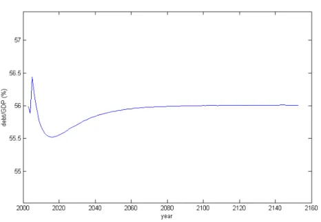
The dynamics of public debt is worth mentioning (see Figure 3). At the initial

(22)

because of the reduction of the fraction of current tax revenue allotted to interest

payments (i.e., a lower ₁). However, as the productivity e¤ects of increasing public investment take place, the debt-to-GDP tends to its stable long-run level,

56%, after some years of undeshooting. In any case, debt to GDP ratio varies in a

very thin interval. The behavior of interest rate is similar, as one can see in Figure

4. In this case, note that the long-run variation ofK and GDP are very close to

each other. Hence, given that r = Y =K;after an initial increase (because during

the transition Y grows faster in the initial periods) the interest rate in the long

run returns to the same level as in the original steady-state.

4.1.2 Public consumption-…nanced expansion of public investment with

higher debt ratio

The second scenario is an augmented version of the previous in which we also allow

for an ad-hoc increase of public debt from 56% of GDP to 60%. Thus, public

investment expansion here is partially …nanced by an increase of public debt. We

assume that the economy is initially in the steady-equilibrium characterized by

the benchmark calibration. Then, …scal policy changes to = (0:79;0:10;0:59),

which implies a new steady-state where Ig

Y = 0:04 and B

Y = 0:60.

Steady-state comparisons suggest that changes in relevant variables are very

close to those observed when debt-to-GDP ratio is kept constant and we increase

public investment share by reducing proportionally government consumption.

Out-put increases a bit less (11%), but private consumption a bit more (11:4%)

The growth gains are lower but very near to 0:4% point as in the …rst

experi-ment. The transitional dynamics is qualitatively identical to previous cases so that

(23)

slightly lower: 3:36%. Finally, transition path of B

Y is displayed in Figure 5 and

shows that convergence is somewhat fast to it is new steady-state, even though

there is a small overshooting at the very beginning of the path.

4.1.3 looser regimes

The “looser regime experiment” consists in changing the calibration of the

bud-getary regime parameters ₀, ₁ and ₂ so that government is explicitly allowed to run public debt so as to …nance public investment (i.e., ₂ > 1). In this case the calibration of relevant parameters required solving a non-linear system of equations

subject to ( 0; 1; 2) 2 [0;5]3;instead of [0;1]3 as in the benchmark calibration.

After using the same numerical methods as before, we get now a …scal policy vector

= ( ₀; ₁; ₂) = (0:95;1:23;1:41).

The experiment, as the previous two exercises, simulates the transition path

from the benchmark economy to an economy with this new …scal regime. The

economic impacts of this policy are negligible. (See …gures 6-7). No variable

increases by more than 0.03% in the long-run, while public debt falls by only

0.33%. The long-run welfare gain is almost zero, 0.004%.

One variation of this scenario, say "looser 2", would be to force the public

in-vestment ratio to increase, in addition to ₂ >1as above. So, in this experiment we …xed Ig_Y to 4% as in the …rst two and, following the same procedure, solve the model

to obtain a new …scal policy vector ;in tis case = ( ₀; ₁; ₂) = (0:95;1:89;2:59). By examining expression (7) it is clear that these parameters imply a signi…cant

boost in the share of investment in total public expenses. However, as we

com-mented before, the higher is the residual fraction of tax revenue to …nance public

(24)

The e¤ect on the economy of this new policy is now relevant. Long-run output

increases by 12%, while private and public consumption by 34% and 4%,

repec-tively. Growth rate, for the next twenty years, is 0.5% above the long run trend.

Although utility increases by 4% in the long run, welfare gains ( x) when taking

into account the transition path is much smaller, only 0.8%. This is so because

imediatialy after the policy switch, Cpfalls by 10% and Cg by 80% (to

compen-sante for the increase inIg), so that in the short-run utility falls. As the converge

is slow, the welfare variation is small. Finally, as expected, the long run level of

public debt is now higher, 12% above the previous level.

Table 1 compares the main results of the four di¤erent …scal regimes. We

present long-run variation of output, private consumption , public capital and

public debt and the two welfare measures that take into account the transition

path. In all cases the benchmark economy is the "before" scenario (Brazil in 2004)

and so the entries represent percentual variation with respect to it.

<<<

Insert Table 1

>>>

With the exception of the "looser" regime in columm three, long-run output

gains are very close to each other in the 3 remaining …scal rules. Same is true

for infrastructure and public debt (although, as expected, in the "public-…nanced

investment with higher debt regime", in columm 2, debt variation is higher).

How-ever, welfare gains in the "public consumption-…nanced regime" clearly dominates

both "looser" regimes. It seems that the use of debt to …nance public investment

does not add much in terms of output gains but, there are a clear disadvantage in

(25)

tax-…nanced investment expansion is inferior to a proportional reduction in public

consumption, keeping government size constant.

4.2 Counterfactual exercises

From 1960 to 1980, public investment as a proportion of GDP averaged more or

less 4% of GDP, with a maximum of 5:3% in 1969. In 2002 and 2003 it was

only 2:2%. At the same time, after ‡uctuating for many years around 25% of

GDP, tax collection in Brazil is above35% of GDP today. Any evaluation of the

impact of the compression of public capital expenditures in the recent past has to

take into account this last fact. Otherwise the output and welfare losses due to

investment cuts will certainly by overestimated. Moreover, although the direction

of the impact is not clear, debt to GDP ratio in the same period went from 33%

to56% in the period.

In this section we perform a group of counterfactual exercises in order to

in-vestigate the impact on product and welfare of the increase in total taxes to 35%

of GDP jointly with a reduction of public investment to 2:2% and an expension

of B=Y to 56%. We assume that tax revenues are distributed as before between

capital and labor, and that , , g, and remained constant over the last two

decades. This is Policy 1 in Table 2 A second issue is to separate the impact of

investment reduction from tax increases. Policy 2 keeps Ig_Y constant and varies tax

collection to35%, while Policy 3 keeps tax rates constant and decreases Ig_Y to2:2%.

In both cases the vector changed accordingly. Results for the 3 experiments are

sumarized in Table 2.

(26)

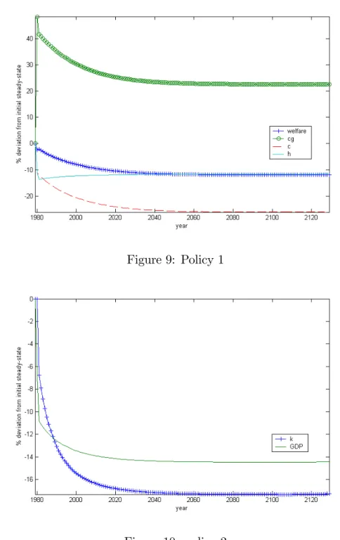
Transition paths for private and public consumption (Policy 1), hours and

wel-fare (utility) are displayed in Figure 8 . Immediately after the policy switch, public

consumption jumps up by more than 40% while hours and private consumption

falls by more than 10% and utility increases slightly. However, the reduction of

public investment (not displayed) has a direct impact on output. As public

cap-ital reduces over time, the marginal productivity of private capcap-ital also falls and

hence private investment and capital too, hurting even more GDP (see …gure 9).

Consequently, both types of consumption fall over time and also utility.

Output loss in the long run is huge, 23:2%, and also steady-state welfare,

almost 16%. However, when taking into account the transition path, welfare loss

is much smaller, 3:17% (= wc), although still very large. This is due to the fact

that utility convergence very slowly to its long-run level, and future is discounted8. Note, however, that the compensated consumption measure of welfare loss, x; is

extremely high, 14:2%.

Growth loss is also sizeable. Instead of growing at 3% on average, as observed

before 1980, the simulated economy grows by only 1:33% ,on average, until 1990

and 1:95%until 2000. How these numbers compares to the actual performance of

the Brazilian economy? From 1980 to 1990 per capita GDP in Brazil grew at0:3%

per year, and in the next decade by 1:2%. Hence, the model under-predicts the

slowdown of Brazilian GDP in the last decades, but explains in any case most of

it. This result is not robust to changes in the calibration of relevant parameters,

as we will see later. In the case of = 0 (no weight to public consumption in

welfare) the matches is almost perfect. We …nd this hypothesis extreme, however,

(27)

given the supply of security, justice, and other services by the government.

In the above simulation we showed that the model calibrated to the observed

changes in tax collection and public investment reduction displayed large welfare

and output losses. We now investigate which one of these factors were more

rele-vant, tax expansion or investment fall. Suppose …rst that from1980 to2004taxes

increased (so that G=Y raises from 25% to 35%) whereas Ig_Y remained constant.

This is Policy 2 in Table 2, and the impact over economic variables are displayed

in …gures 10 and 11. The welfare cost of this policy change was estimated to be

2:44%;as proportion of present value of output, or 11:1% when measured by x:

The increase in k and h causes an immediate reduction on hours worked and

private investment (not displayed), given that the net return of both factors were

reduced. GDP drops down with hours and later with private capital. As we …xed

public investment ratio, Kg also falls because tax collection was reduced. In the

long run, output would be14:4% smaller than it would be in the previous regime.

The impact on private consumption is also signi…cant (close to20%) and it o¤sets,

when considering utility, the expansion of Cg and the reduction in hours worked.

The estimated reduction in growth of this policy was 1.46% in the …rst ten years

and 0.76% in the nineties.

Finally, suppose that tax rates remained at the levels of 1980 so that G/Y is

kept constant, but adjusted so that Ig_Y in equilibrium falls from4%to2:2%. The

variation of GDP and private capital is smaller than in the previous experiment,

11%in this case. At the same time, while in the previous case private consumption

in the long-run would be25%smaller after the policy change, it now falls less than

7%. AsCg initially increases and hours worked falls, the decrease in utility is now

(28)

value terms is only 0:82% (= wc). This is one third of the loss estimated in the

previous case. Likewise, we foundx= 3:69%:

In summary, the simulations indicate that the welfare and growth costs of the

increase of tax collection in Brazil were far greater than those caused by the

re-duction of public investment. In the last case, average growth rate in the ten years

after the policy change falls by only 0:4 points, while the expansion of taxation

alone would have induced a drop of1:5points, more than half the observed growth

slowdown in the eighties. Although the sum of the welfare loss implied by Policies

2 and 3 overpredicted slightly that of Policy 1, due to non-linearities of the model,

the observed increase in taxes explains almost 75% of the welfare loss and, at the

same time, 56% of the output loss9_.

5 Alternative Scenarios: the model without debt

One problem of the above simulations is that, given the number of variables

in-cluded and especially the procedures involved with public debt, it takes from …ve

to six hours to run one single experiment. This of course limits sensitivity analisys

and robustness checks. Given that we are running several of these experiments, the

computational time implied render these sensitivity tests unfeseable in the present

set up10_.

One possible (partial) solution is to run experiments without debt. By

simpli-9_{As we will see in the next section, the impact of debt variation is very small. Replicating} Policy 1 with no variation in debt found almost the same output loss and slightly higher welfare loss.

(29)

…ying considerably the model and, consequently, computer programs, simulations

in this case last a very small fraction of the time of the complete program with

public debt(at most …ve minutes). Of course, this would be a problem if results

were too di¤erent from each other. However, this is not the case. For instance, in

the very …rst model simulation, labeled "public consumption-…nanced expansion of

public investment", instead of increasing by11:5%;GDP now raises by10:5%;while

in both cases Kg doubles and Cg increases by 4%. Moreover, from Figure 12 it

is clear that transition paths are also very similar (compares to Figure 1). This is

also the case for Policy 1 and the other experiments.

In very few cases there are any signi…cant di¤erences and they all refer to

welfare variations. In this sense, we opt to present a number of sensitivity exercises

using the model without debt as we believe the result are very close to those of the

model with public debt. Moreover, in one case (the "tax-…nanced investment")

the simulations did not converge in the full model, so that we present below the

results of this …scal regime when using the model without public debt. In this

case we compare results with those of the "consumption-…nanced" regime without

public debt. This is done before the sensitivity analisys.

We propose an arti…tial economy where the utility function, technology and

…rm´s problem is the same as the above, but with some relevant di¤erences. The

households’ budget constraint is now given by:

(30)

By ruling out debt …nancing, government budget constraint reads:

Cgt+Igt=Gt = krtKt+ hwtHt: (19)

For the sake of simplicity, we assume that government follows a simple and

known rule to split its expenditures between consumption and investment:

Cgt = (1 )Gt; (20)

Igt= Gt; (21)

where0 1. Therefore, in our set-up …scal policy is represented by the triple

( k; h; ). Simulations, transition paths and welfare calculations follow closely

those discussed in Section 3, and the calibration procedures are presented in an

appendix.

5.1 Long-run relationships

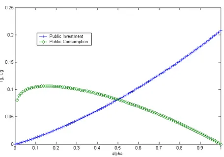
The relativity simplicity of this model also allows us to better understand the

economic e¤ects of public investment. Steady-state is signi…cantly in‡uenced by

the proportion of public investment in total public expenditures. If we increase ,

government consumption decreases, while public capital rises (see …gure 13). Note

that public consumption increases with lower values of . In this case the

produc-tive impact of public investment o¤set the negaproduc-tive impact of lower consumption

share, so that the level of Cg goes up.

This fact clearly presents a trade-o¤ when is raised. In the one hand, welfare

(31)

. On the other hand, welfare increases with Kg; as it has a positive e¤ect on

output and consumption. This fact is rarely taken into account in the analysis of

the welfare and productive impact of infrastructure. Depending on the weight of

public consumption on the government budget and how much agents value Cg,

it may be the case that, although output always increase with (see …gure 14),

welfare may improve with reductions of public investment.

In …gure 15 below we can see clearly that the positive e¤ects of Kg on GDP

dominates up to a certain level of , increasing income and private consumption

su¢ciently to raise steady-state welfare. After some threshold , that depends of

parameters such as and , welfare tends to decrease with expansions of public

investment.

5.2 A new experiment: tax …nanced investment

The simplicity of the model without debt allowed us to to perform one extra

ex-periment that we could not do in the original model due to the limitations of the

simulation procedures. We want to investigate the economic impact of using an

ex-pansion of tax collection to …nance the increase of public investment from 2.2% to

4% of GDP. In this sense, we keep consumption as a share of GDP constant but

in-crease government size. In other words, while in the "public consumption-…nanced

expansion of public investment" experiment we keep G=Y constant and decrease

Cg=Y to …nanceIg=Y, nowCg=Y is kept constant andG=Y rises accordingly (to

37% from 35%).

The gains now are smaller than those of simple switching Cg for Ig, although

(32)

bench-mark no-debt calibration) which is 3 points below that of the consumption-…nanced

experiment. Likewise, the welfare gain in terms of consumption compensation is

4.04%, 2 points smaller. For the following 20 years the economy would grow at a

rate 0.2% above its long-run trend, althouth there is an absolute reduction of GDP

immediately the implementation of the new policy, because of the rising taxes, as

one can see from Figure 16. The trajectory of most variables, in any case, are very

close to those of the consumption-…nanced investement expansion rule.

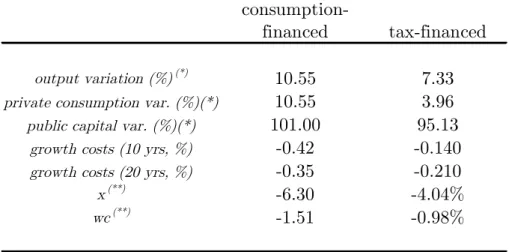
Table 3 compares the main results of the 2 di¤erent …scal regimes, the

"pub-lic consumption-…nanced expansion of pub"pub-lic investment" and the "tax-…nanced

expansion of public investment".

<<<

Insert Table 3

>>>

It is not surprising that the latter dominates the former in terms of long-run

output growth and also in terms of welfare gains. Both experiments expand public

investement by the same amount, but when using taxes the government increases

alocative distortions in the economy, while in the "consumption-…nanced" …scal

rule it does not do so, as taxes remain the same.

5.3 Sensitivity Analysis ( and )

We adopted in the above experiments a conservative calibration for the parameter

; picking a medium to lower value among the many estimates in the literature.

We think this was the most reasonable choice, otherwise we could be blamed for

arti…cially boosting the gains of infrastructure investment. However, it is

(33)

is employed. In the case of the counterfactual exercises we would get a better

assessment of the importance of taxation vis-à-vis infrastructure expenditures for

the growth slowdown of the last two decades. In this sense we redo all the previous

experiments with = 0:15 and 0:20: These values are close to the estimations in

Calderón and Servén (2003), for instance, and, in particular, = 0:15is the value

used by Rioja and Glomm (2003).

At same time, previous experiments have assumed that private and public

consumption are imperfect substitutes, i.e., < 0:5. This is rather unfortunate

assumption for some authors, who claim that public consumption is pure waste,

with zero utility impact. In order to assess how the results would change we

consider the extreme cases of = 0 and 1. The former value implies that public

consumption does not enter the utility function, while the latter means private

and public consumption are now perfect substitutes.

First we consider the experiment of increasing public investment to GDP ratio

from 2:2% to 4%, labelled "public consumption-…nanced expansion of public

in-vestment" (Table 4). As with all sensitivity analysis simulations, no qualitatively

distinct dynamic behavior with respect to the variables along the transition path

were observed, so that we opted not to present pictures. Focusing on the

steady-state, main results are the following. If we hold constant at 0:09, when = 0

output increases by 9.2% in the long-run, instead of 10.5% as in the benchmark

case, a rather small change (see Table 4). At the same time, long run welfare(wc)

falls marginally from 1.51% of GDP to 1.27%. On the other hand, growth gains

are smaller, falling to 0.31% during the …rst 10 years (as opposed to 0.42%). Note

that the growth costs for the case = 1almost match the actual growth slowdown

(34)

Similarly, results with respect to couterfactual "Policy 3" - keeping taxes

con-stant at their 1980 level and reducing infrastructure investment from4:4%to2:2%

- do no change much, as one can see from Table 7. This is expected given that

both groups of simulations are close to each other. Note also that, if agents value

public consumption as much as private consumption ( = 1), the welfare and

growth gains of expanding government capital expenditures would increase with

respect to those observed in the benchmark economy.

There are sizable di¤erences with respect to the "Policy 1" and "Policy 2"

counterfactual experiments. In both cases taxes decreases, but in the former

in-frastructure also falls while in the latter it remains constant at the 1980 level. In

Policy 1, as one can see from Table 5, the fall of output when = 0is much smaller

than when = 0:5( 13% in the …rst case and 22% in the second, respectively). In

contrast, welfare loss are larger in the …rst case. There is no puzzle here because

the increase in public consumption observed in both experiments does not a¤ect

utility by construction when = 0:Hence, although Cg raises by only12% in the

long run when = 1; as opposed to 36% when = 0; consumers do not bene…t

from the latter. In the former the increase in government current expenses

par-tially compensates the loss in private consumption, and so welfare loss is smaller.

The same reasoning works for Policy 2 displayed in Table 6 .

The big picture with respect to di¤erent utility function parametrizations is

that output cost of tax variations are higher when agents value public consumption,

but welfare losses smaller. In contrast, there are no relevant di¤erences with respect

to changes in the proportion of capital expenditures in the government budget.

If is held constant, higher values of are associated with greater levels of

(35)

Looking at the transition paths, the higher is , the greater is the growth in

the short-run (although not by much). The transitional dynamics of simulations

respecting policies 1, 2 and 3 do not display any surprising change, as already

stressed. A complete understanding of how the model has performed under the

sensitivity analysis exercises follows from the inspection of Tables 4-7. In the case

where taxes are held constant, but Ig=Y falls to 2.2% (Policy 3) the output loss

when = 0:2 is more than twice as large as in the benchmark economy - as the

impact of the decreased Kg is now appli…ed - while welfare loss is three to four

times larger, depending on the measure used.

6 Concluding Remarks

Results in this paper indicate that the compression of capital expenditures

ob-served in the recent past may have played a signi…cant role in the growth slowdown

of the Brazilian economy after the eighties. Moreover, if public investment ratio

return to its level of two decades ago, the country would converge to a balanced

growth path in which GDP would be11%greater than today’s path. Growth rate

would be 0:5 points above its after war average for at least 20 years. Welfare, in

present value, would also improve, but in a smaller scale. This outcome could be

achieved either by increasing permanently public debt from 56% of GDP to 60%

or by reducing proportionally government consumption in favor of investment,

keeping everything else constant.

The model was also used to investigate how much the deterioration of

in-frastructure conditions can explain the recent trajectory of the Brazilian economy.

(36)

aggres-sive increase of taxation after the eighties was considerably more detrimental to

growth than public investment compression.

This should not surprise us. Tax base in Brazil was for many years 25% of

GDP, but it is now more than35%. Our calibration found that the corresponding

increase in the capital tax rate was39:8%, so that the negative impact on its return

was strong, reducing the incentives to invest. The same is true with respect to the

labor income taxation.

The lagging of infrastructure expenditure also a¤ects returns, but our

simula-tions showed that the growth and welfare impact were smaller. The main reasons

are, in the one hand, that the impact is mostly felt in the long run, given that

public capital is a stock. In the other hand,Kg enters in the production function

to the power of , so that the impact of its variation on returns is drastically

reduced (to the power of 0:09, in the present calibration).

The question of enlarging …scal space to infrastructure investment has to take

into account these observations. The simulations in the article, summarized in

Tables 1 and 3, allow one to conclude that the reduction of public consumption to

…nance the necessary expansion of public capital investment is the most desirable

…scal scheme among those we examined. The use of debt to …nance investment

reached mixed results and tax …nanced investment was dominated in all dimension

by the consumption-…nanced investment rule. As we stressed in the introduction,

there is certainly room for this type of policy in Brazil, especially when we take

into account the recent increase of government size. Moreover, in all simulations

the expansion in investment is relatively modest (although not the bene…ts) and

(37)

References

[1] Ai, C. and S. Cassou (1995), “A Normative Analysis of Public Capital,”

Applied Economics, v.27, pp. 1201-1209.

[2] Afonso, J. R. (2004). “Managing Fiscal Space in Brazil.”manuscript.

[3] Araújo, C. H. V. and P. C Ferreira. (1999). “Reforma Tributária, Efeitos

Alocativos e Impactos de Bem-Estar.” Revista Brasileira de Economia, v.53,

pp.133-166.

[4] Ascahuer, D. (1985). “Fiscal Policy and Aggregate Demand.”American

Eco-nomic Review, v.75, pp. 117-127.

[5] Aschauer, D. (1989) “Is Public Expenditure Productive?,” Journal of

Mone-tary Economics, v.23, pp. 177-200.

[6] Ba¤es, J. and A. Shah(1998) “Productivity Of Public Spending, Sectorial

Al-location Choices, And Economic Growth,” Economic Development and

Cul-tural Change, v.46, pp. 291-303.

[7] Barro, R. J. (1981). “Output E¤ect of Government Purchases.” Journal of

Political Economy, v.89, pp.1086-1121.

[8] Barro, R. J. (1990). “Government Spending in a Simple Model of Endogenous

Growth.”Journal of Political Economy, v.98, pp. S103-S125.

[9] Barro, R. J. and X. Sala-i-Martin, (1993). “Public Finance in Models of

(38)

[10] Calderón, C. and L. Servén (2003) “The Output Cost of Latin America’s

In-frastructure Gap,” In W. Easterly and L. Servén (eds.) The Limits of

Stabi-lization: Infrastructure, Public De…cits, and Growth in Latin America,

Stan-ford University Press and the World Bank.

[11] Canning, D. and M. Fay (1993) “The E¤ect of Transportation Networks on

Economic Growth,” manuscript, Columbia University.

[12] Christiano, L.; M. Eichenhaum. (1992). “Current Real Business Cycle

Theo-ries and Aggregate Labor Markets Fluctuations.”American Economic Review,

v.82, pp. 430-450.

[13] Cooley, T. F. and G. D. Hansen (1989) “The In‡ation Tax in a Real Business

Cycle Model,” American Economic Review, v.79, pp. 733-748.

[14] Du¤y-Deno, K. and R.W. Eberts (1991), “Public Infrastructure and Regional

Economic Development: a Simultaneous Equations Approach,” Journal of

Urban Economics, v.30, pp. 329-343.

[15] Easterly, W and S. Rebelo (1993) “Fiscal Policy and Economic Growth: an

Empirical Investigation,” Journal of Monetary Economics, v.32, pp. 417-458.

[16] Evans, P. and G Karras. (1996). “Private and Government Consumption with

Liquidity Constraints.”Journal of lnternational Money and Finance, v.15, pp.

255-266.

[17] Ferreira, P. C. (1993). Essays on Public Expenditure and Economic Growth.

(39)

[18] Ferreira, P. C., and J. V. Issler (1998) “Time Series Properties and Empirical

Evidence of Growth and Infrastructure.” Revista de Econometria, v.18, pp.

31-71.

[19] Ferreira, P.C. and T. Maliagros (1998) “Impactos Produtivos da

Infra-Estrutura no Brasil – 1950/95”, Pesquisa e Planejamento Econômico, v.28,

pp.315-338.

[20] Ferreira, P. C. (2001). “A Note on Growth, Welfare and Public Policy.”Revista

de Economia Política, v. 21, pp. 101-116.

[21] Ferreira, P. C. (2004). “Infrastructure and Public Investment in Brazil: Some

Stylized Facts.” manuscript, EPGE-FGV.

[22] Ferreira, P.C. and C. H. V. Araújo (2004) “Fiscal Space for Infrastructure

Investment in Brazil,” manuscript, EPGE-FGV.

[23] Glomm, G., and B. Ravikumar. (1997). “Productive Government

Expendi-tures and Long-Run Growth.” Journal of Economic Dynamics and Control,

v.21, pp. 183-204.

[24] Gramlich, E. M. (1994). “Infrastructure Investment: A Review Essay.”

Jour-nal of Economic Literature, v.32, pp. 1176-1796.

[25] Greiner, A. and W. Semmler. (2000). “Endogenous Growth, Government Debt

and Budgetary Regimes.”Journal of Macroeconomics, v.22, pp. 363-384.

[26] Hansen, G., and E. Prescott (1995) “Recursive Methods for Computing

Equi-libria of Business Cycles Models,“ in Cooley. T. (org.) Frontiers of Business

(40)

[27] Hansen, L. P. (1982). “Large Sample Properties of Generalized Method of

Moments Estimators”. Econometrica, v.50, pp. 1029-1054.

[28] Holtz-Eakin, D. (1992), “Public Sector Capital and Productivity Puzzle,”

NBER Working Paper no. 4122.

[29] Hulten, C. and R. Schwab (1992), “Public Capital Formation and the Growth

of Regional Manufacturing Industries,” National Tax Journal, v.45, pp.

121-143.

[30] Ratner, J.(1983) “Government Capital and the Production Function for U.S.

Private Output,”Economic Letters, v.13, pp. 213-217.

[31] Rioja, F. and G. Glomm (2003) “Populist Budgets and Long Run Growth,”

manuscript, Georgia State University.

[32] Turnovsky, S. J.(1997). “Fiscal Policy in a Growing Economy with Public

Capital.” Macroeconomic Dynamics, v.1, p.615-639.

[33] Turnovsky, S. J.(2000). Methods of Macroeconomic Dynamics. 2nd. edition.

(41)

7 Figures and Tables

Figure 1: Transition path of capital and GDP ("consumption-…nanced" policy)

Figure 2: Transition path of consumption, hours and utility

(42)

Figure 3: Debt/GDP ratio after permanent increase in Ig/GDP

("consumption-…nanced" policy)

(43)

Figure 5: Transition path of Debt/GDP ("consumption-…nanced" policy with

debt increase)

(44)

Figure 7: looser regime

(45)

Figure 9: Policy 1

(46)

Figure 11: Policy 2

Figure 12: Transition paths of GDP and capital (no-debt model,

(47)

Figure 13: Steady-state levels of public consumption and public investment

(48)

Figure 15: Steady state utility levels

(49)

consumption-financed consumption-financed + Change Debt Looser Regime Looser Regime 2

output variation (%)(*) 11.49 11.00 0.003 12.09

private consumption var. (%) 11.14 11.56 12.82 34.95

public capital var. (%) 99.23 95.19 0.00 105.85

public debt var. (%) 11.53 18.96 -0.22 12.08

growth costs (10 yrs, %) -0.46 -0.43 0.000 -0.36

growth costs (20 yrs, %) -0.38 -0.36 0.000 -0.50

x(**) -3.57 -3.36 -0.004 -0.77

wc(**) -0.83 -0.83 -0.001 -0.31

'(*)

Steady-State.

(**)

Takes into account transition and is expressed in percentual terms.

Table 1 - Fiscal Rules for Investement Financing

Policy 1

(tax and Ig change)

Policy 2

(only tax changes)

Policy 3 (only Ig changes)

output variation (%)(*) -23.23 -14.40 -11.11

private consumption var. (%)(*) -32.73 -25.37 -6.31

public capital var. (%)(*) -57.38 -15.10 -51.10

public debt var. (%)(*) 26.93 41.58 50.94

growth costs (10 yrs, %) 1.77 1.54 0.43

growth costs (20 yrs, %) 1.05 2.24 0.34

x(**) 14.24 11.11 3.69

wc(**) 3.17 2.44 0.82

'(*)

Steady-State.

(**)

(50)

consumption-financed tax-financed

output variation (%)(*) 10.55 7.33

private consumption var. (%)(*) 10.55 3.96

public capital var. (%)(*) 101.00 95.13

growth costs (10 yrs, %) -0.42 -0.140

growth costs (20 yrs, %) -0.35 -0.210

x(**) -6.30 -4.04%

wc(**) -1.51 -0.98%

'(*)

Steady-State. (**)

(51)

0.09 0.15 0.2

output variation (%)(*) 9.19 17.64 26.89

growth costs (10 yrs, %) -0.31 -0.51 -0.68

0 growth costs (20 yrs, %) -0.29 -0.51 -0.69

x(**) -7.25 -12.82 -17.99

wc(**) -1.27 -2.50 -3.93

growth costs (10 yrs, %) -0.42 -0.62 -0.78

0.5 growth costs (20 yrs, %) -0.35 -0.56 -0.75

x(**) -6.30 -12.04 -17.35

wc(**) -1.51 -3.28 -5.39

growth costs (10 yrs, %) -0.49 -0.69 -0.84

1 growth costs (20 yrs, %) -0.39 -0.60 -0.79

x(**) -6.03 -11.85 -17.23

wc(**) -1.84 -4.18 -7.05

'(*)

Steady-State.

(**)

Table 4 - Consumption-Financed - Sensitivity Analysis

φ

(52)

0.09 0.15 0.2

growth costs (10 yrs, %) 0.62 0.74 0.83

0 growth costs (20 yrs, %) 0.47 0.63 0.76

x(**) 31.61 40.23 49.23

wc(**) 5.70 8.33 11.67

growth costs (10 yrs, %) 1.59 1.72 1.82

0.5 growth costs (20 yrs, %) 0.97 1.14 1.29

x(**) 19.65 28.64 38.10

wc(**) 4.91 8.33 12.87

growth costs (10 yrs, %) 2.25 2.38 2.49

1 growth costs (20 yrs, %) 1.31 1.50 1.65

x(**) 15.29 24.76 34.78

wc(**) 4.90 9.35 15.43

'(*)

Steady-State.

(**)

Table 5 - Couterfactual Policy 1 - Sensitivity Analysis

φ

(53)

0.09 0.15 0.2

growth costs (10 yrs, %) 0.44 0.45 0.45

0 growth costs (20 yrs, %) 0.24 0.25 0.26

x(**) 22.42 22.95 23.49

wc(**) 3.86 4.37 4.95

growth costs (10 yrs, %) 1.32 1.34 1.36

0.5 growth costs (20 yrs, %) 0.70 0.73 0.76

x(**) 12.49 13.92 15.35

wc(**) 2.93 3.68 4.56

growth costs (10 yrs, %) 1.92 1.96 1.98

1 growth costs (20 yrs, %) 1.01 1.06 1.10

x(**) 8.75 10.81 12.87

wc(**) 2.62 3.68 5.00

'(*)

Steady-State.

(**)

Table 6 - Counterfactual Policy 2 - Sensitivity Analysis

φ

(54)

0.09 0.15 0.2

growth costs (10 yrs, %) 0.18 0.30 0.39

0 growth costs (20 yrs, %) 0.23 0.38 0.51

x(**) 7.54 14.11 20.94

wc(**) 1.45 3.10 5.26

growth costs (10 yrs, %) 0.29 0.40 0.49

0.5 growth costs (20 yrs, %) 0.28 0.43 0.56

x(**) 6.37 12.98 19.86

wc(**) 1.50 3.55 6.28

growth costs (10 yrs, %) 0.37 0.48 0.56

1 growth costs (20 yrs, %) 0.32 0.47 0.60

x(**) 5.79 12.46 19.39

wc(**) 1.63 4.09 7.44

'(*)

Steady-State.

(**)

Table 7 - Counterfactual Policy 3 - Sensitivity Analysis

φ

µ

A

Calibration and Simulation Procedures of the

Model Without Public Debt

We follow the model with public debt and use as benchmark values = 0:5

(55)

We will use in the sensitivity analysis equal one and zero and equal 0.15 and

0.2.

In the model, interest rate is also determined by the marginal productivity of

capital: r = Kg H_K (1 ). This equation can be rewritten as:

= rK Y :

From the National Accounting data we have that K

Y = 2:98and current real interest

rate is r= 0:1, so that we set capital share to 0:298:11

Depreciation rate is = g = 0:0656, following in the …rst case Araújo and

Ferreira (1999), and setting g for symmetry.

With respect to the …scal policies parameters, there is evidence that taxes levied

on capital correspond to 8:01% of GDP when we include investment taxes12_{. In}

this sense we have:

k = 0:0801

Y

rK = 0:2688:

Similarly, using the fact that labor income taxes represent 26:98% of GDP13_{, we}

obtain:

h = 0:2698

Y

wH = 0:3844:

11_{This value is a bit below the international evidence (see Gollin (2003)) and well below} Brazilian National Accounting data. In the case of the latter, however, we should not be too worried as they do not take into account a number of imputations that ends up overestimating capital share.

12_{This calculation is performed by using the decomposition of total taxes into its components} as presented in Araújo and Ferreira (1999).

13_{Note that our model only allows for capital and labor taxes. In this sense it was} proportion-ally transferred to labor taxes the consumption taxes and to capital taxes the taxes on investment, in order to obtain the observed tax ratio of the Brazilian economy, 35%_{. As our experiments}

(56)

The share of public investment expenditure, , is ideally set by taking into account

that total taxes over GDP are nearly equal to35% and that the public investment

rate (Ig_Y ) is 2:2% (Ferreira (2004)). Thus:

0:022 = Igt Yt

= Gt Yt

= 0:35

) = 0:0628:

Intertemporal discount factor, , is found by using the long-run equation

de-rived from the …rst order condition of the model, as before:

= 1

1 + (1 k)r