Exact linearization of an induction machine with rotoric flux orientation

(1)

Vol. 5, No. 2, November 2008, 217-227

Exact Linearization of an Induction Machine

with Rotoric Flux Orientation

Abderrahim Bentaallah

1

, Abdelkader Meroufel

1

,

Abdelber Bendaoud

1

, Ahmed Massoum

1

,

Mohamed Karim Fellah

1 Abstract: In this paper, we present the linearization control of an asynchronous machine. It allows decoupling and linearization of the system without including flux orientation. This non-linear control (NLC) applied to the asynchronous machine breaks up the system into two linear and independent mono systems. The speed and the Id current controls are carried out by traditional regulators PI. A qualitative analysis of the evolution of the principal variables describing the behaviour of the global system (IM-control) and its robustness is developed by several tests of digital simulation in the final stage. Numerous tests have been performed under Simulink/Matlab to show the control system performances.

Key words: Induction machine, Non-linear control, Field oriented control.

1 Indroduction

In recent years, asynchronous motors are more commonly used in the control

processes that require different speeds and positions.

The application of techniques of modern automation in electric machines control provides obtaining very high performances. The research in respective field is focused on the application of these techniques in the machine control.

In this paper, the application of the control by Linearization Feedback to an asynchronous machine [1–3] is the matter of our interest.

This technique enables us to linearize and decouple the system by using the differential geometry, whereupon the control by pole placement is applied to system. Finally, the control structure is tested by simulation on the linearized model of machine.

2 State Feedback Exact Linearization

Let us consider the class of the nonlinear dynamic system in the form:

1

(2)

( )

1

1 1

, m

i i

i

m m

x f x g x u

y h x

y h x

=

= +

=

∑

(1)

where _x∈_Rn,

( )

1 , , m

h x … h x and f x

( )

,g x₁

( )

,…, g_m

( )

x are differentiable

vector functions of suitable size.

Further, co-ordinates transformation and a

nonlinear state feedback which linearize the system are to be found.

Thus let us consider a static nonlinear state feedback of the form:

( )

x

( )

x

= +

u α β v, (2)

whereβ

( )

x = β⎡_⎣ _ij

( )

x ⎤_⎦; for i=1,…,m and j=1,…,m, is non singular and

( )

T

1 , , m

x x x

α = ⎡α_⎣ _… α ⎤_⎦

.

The exact linearization of system (1) with output h x_i

( )

has to provide the

solution to

nonlinear state feedback (2) and the co-ordinates transformation:

( )

x 1

( )

x , , n

( )

x = = ⎡Φ_⎣ Φ ⎤_⎦

z Φ … this put the closed loop system in the canonical

form of Brunowsky [4, 5],

= + =

z Az Bv

y Cz (3)

where v is the new control vector.

With A=diag

( )

A , B=diag

( )

B , and C=diag( )C :

0 1 0 0 0 1

0 0 1 0 0 0

; ; 0 .

0 1 0

0 0 1 0

⎡ ⎤ ⎡ ⎤ ⎡ ⎤

⎢ ⎥ ⎢ ⎥ ⎢ ⎥

= = =

⎢ ⎥ ⎢ ⎥ ⎢ ⎥

⎣ ⎦ ⎣ ⎦ ⎣ ⎦

i i i

A

B

C (4)

In relation to the equations of state (1) we define the vector relative degree

{

r₁,…,r_m

}

. The system given by (1) has a vector relative degree

{

r1,…,rm

}

in a point x0 if and only if:

1. The product

( )

0 k

gj f i

(3)

for 1≤ ≤i m, 1≤ ≤j m and fork< −r₁ 1. L h x_f

( )

is the Lie derivative

of the function h x

( )

according to the vector f.

2. The decoupling matrix

( )

1

,

( ) _gi rj_f _j i j

x = ⎣⎡L L − h x ⎤_⎦

A (6)

is non-singular at the point x₀ for 1≤ ≤i m and 1≤ ≤j m. The system is exactly linarizable if and only if r₁+ +r_m=n, i.e. after diffeomorphism and looping the system will consist of m linear and decoupled subsystems.

3 Nonlinear Model of the Asynchronous Machine

The machine model, in the selected reference frame d-q in such manner that rotor flux has a null component according to the q axis (Φ = Φ Φ =_dr _r, _qr 0), is

given by the following states equations:

( )

= +

X F X GU (7)

with: 1 2 3 4 ds qs ds x i x i x x ⎡ ⎤ ⎡ ⎤ ⎢ ⎥ ⎢ ⎥ ⎢ ⎥ ⎢ ⎥ = =

⎢ ⎥ ⎢Φ ⎥ ⎢ ⎥ ⎢ _Ω ⎥ ⎣ ⎦ ⎣ ⎦

X , ds

qs U U ⎡ ⎤ = ⎢ ⎥ ⎣ ⎦

U ,

( )

1 2 3 4 f x f x f x f x ⎡ ⎤ ⎢ ⎥ ⎢ ⎥ = ⎢ ⎥ ⎢ ⎥ ⎢ ⎥ ⎣ ⎦

F X , G= ⎡_⎣g x₁

( )

g₂

( )

x ⎤_⎦,

(8)

( )

(

)

T

1 1 / s 0 0 0

g x = ⎡_⎣ σL ⎤_⎦ , g₂

( )

x = ⎡_⎣0 1 /

( )

σL_s 0 0⎤_⎦T,

2 2

2

1 2 1 2 3 2 4

3 2

1 2

2 2 2 3 4 1 4

3

3 1 3

4 2 3 4

1 1

1

,

s r

r r ds

s r s S r s

s r

r qs

s r s S r r s

r r

r

R M R M x

x x R x R x x u

L L L L L x L

R M R M M x x

x x x x R x x u

L L L L L L x L

R R

x Mx x

L L

C f M

x x x x

J L J j

⎛ ⎞

= −_⎜ + _⎟ + + + +

σ σ σ σ

⎝ ⎠

⎛ ⎞

= −_⎜ + _⎟ − − + +

σ σ σ σ

⎝ ⎠

= −

= − −

(9)

(4)

( )

2 2 2

1 2 1 2 3 2 4

3 2

1 2

2 2 2 3 4 1 4

3

3 1 3

4 2 3 4

1 . . 1 , s r r r

s r s S r

s r

r

s r s S r r

r r

r

R M R M x

f x x R x R x x

L L L L L x

R M R M M x x

f x x x x R x x

L L L L L L x

R R

f x Mx x

L L

C f M

f x x x x

J L J j

⎛ ⎞

= −_⎜ + ⋅ _⎟ + ⋅ + +

σ σ σ

⎝ ⎠

⎛ ⎞

= −_⎜ + _⎟ − − +

σ σ σ

⎝ ⎠ = − = ⋅ − − (10) with 2 2 2

1 , s ,

s r s s r s r

R R M

M _r

L L L L L

M K

L L

σ = − λ = +

σ σ =σ .

The electromagnetic torque developed by machine is given by:

3 2

elm dr qs

r

M

C I

L

= Φ . (11)

3.1 The output choice

The output choice is related to the objectives of control. As outputs x₃ (d-axis rotor flux components) and x₄ (speed) are chosen [6, 7]:

( )

1

( )

_{( )}

3

2 4

h x x

x

h x x

⎡ ⎤ ⎡ ⎤ =_⎢ _{⎥ ⎢ ⎥}= ⎣ ⎦ ⎣ ⎦

Y . (12)

3.2 Input/Output linearization

The determination of the relative degree allows the nonlinear system to

check the admittance of an input/output linearization:

a) Degree relating to the output Y x₁

( )

:

( )

1 1 1

2

1 1 1 1 .

f

f g f ds

Y x h x L h x

Y x h x L h x L L h x u

= =

= = + (13)

The relative degree associated to Y x₁( ) is r₁=2.

(5)

( )

2 2 2

2

2 2 2 2 .

f

f g f qs

Y x h x L h x

Y x h x L h x L L h x u

= =

= = + (14)

The relative degree associated toY x₂

( )

is r₂ =2. With

( )

1 1

1 1 3

f

r r

f

r r

L h x h x

R R

L h x Mx x

L L

=

= −

( )

2

2 2

1 1 3 2 4 1 3

3

1

r r r r

f r ds

r s r s r r

R MR x R R

L h x M x x R x x u Mx x

L L L x L L L

⎛ ⎛ ⎞ ⎞

= ⎜_⎜ ⎜−λ +_σ + + +_σ ⎟− − ⎟_⎟

⎝ ⎠

( )

2 2

2 2 3

1 f

r f

r

L h x h x

C M

L h x x x

J L J

=

= −

( )

2 1 2

2 2 3 4 1 4 3 2 1 3

3

. qs

r r r

f

r s r r s r r

u

MR x x R M R

M M

L h x x x x x x x x x x

JL L L L x L L L

⎛ ⎞ ⎛ ⎞

= _⎜−λ − − + + _⎟ + _⎜ − _⎟

σ σ _⎝ _⎠

⎝ ⎠

With

( )

(

( )

)

( )

(

( )

)

2

1 1 2

2

2 3 2 2 3 .

r f r f r R

L h x Mf x f x L

M

L h x x f x x f x JL

= −

= +

(15)

The choice of these outputs leads to a complete linearization of order four (r₁+ =r₂ N=4), where N is the system order [8, 9].

3.3 Diffeomorphism transformation

The change of nonlinear co-ordinates is given by the equations system according to [10–12]:

( )

1 1 3

2 1 3

3 2 4

4 2 4 .

f

z h x x

z L h x f x

z h x x

z L h x f x

= =

(16)

(6)

( )

1 2 2

2 1 1 1

3 4 2

4 2 2 2.

f g f ds

f g f qs

z z

z L h x L L h x u v

z z

z L h x L L h x u v =

= + =

=

= + =

(17)

3.4 Nonlinear control law

To have a complete input/output linearization of order four in closed loop, it is necessary to apply the nonlinear state feedback, [13, 14].

1 1

2

( )x v ( )x v

− ⎡⎡ ⎤ ⎤

= _⎢_{⎢ ⎥}− _⎥ ⎣ ⎦

⎣ ⎦

U D A , (18)

where

3

0

( ) 0

r

s r

MR L L x

Mx J L L

⎡ ⎤

⎢_σ ⎥

⎢ ⎥

=

⎢ ⎥

⎢ _σ ⎥

⎣ ⎦

D . (19)

The decoupling matrix D( )x is not singular,det

[

D( )x

]

≠0, where:

2 3

1 1

2 2 3

0 ( )

0

( ) , ( )

( ) f s r

f r

r x J L L

x J

MR x

R

L h x x

L h x

− ₌ σ ⎡⎢ ⎤⎥ _{= ⎢}⎡ ⎤

⎥

⎢ ⎥ _⎢_⎣ _⎥_⎦

⎣ ⎦

D A . (20)

The application of the law (18) to system of equation (17) leads to the linear model (21) Fig. 1

1 2, 2 1, 3 4, 4 2.

z =z z =v z =z z =v (21)

Fig. 1 – Decoupled linear system.

The linearization and

decoupling

for induction machine (IM) model is obtained by an appropriate selection of the control input _[ _]T

ds qs

u= u u in the

(7)

2

1 1

1

2

2 2

( ) ( )

( )

ds f

qs f

u L h x v

x

u L h x v

− ⎡− + ⎤

⎡ ⎤

= _⎢ _⎥

⎢ ⎥ ₋ ₊

⎢ ⎥

⎣ ⎦ D ⎣ ⎦. (22)

4 Trajectory Imposition Control

To follow reference trajectory of flux (z₁_ref) and speed (z₃_ref) with a certain

dynamic, one imposes to the linearized system stable poles satisfying the desired performances (polynomial of Hurwitz). The inputs v v₁, ₂ can be calculated by [15, 16]:

(

)

(

)

(

)

(

)

1 11 1 1 12 1 1

2 21 3 2 22 3 3 3 .

ref ref ref

v k z z k z z z

= − + − +

= − + − + (23)

The error equations become:

1 12 1 11 1

2 22 2 21 2

0

0.

e k e k e

+ + =

+ + = (24)

with e₁=z₁_ref −z₁ and e₂=z₃_ref −z₃.

The coefficients k_ij (i=1, 2; j=1, 2) are selected to satisfy the polynomial

of Hurwitz:

2 11 12

2 21 22

0

0.

k k s s

k k s s + + =

+ + = (25)

5 Simulation

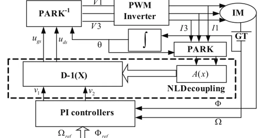
The global nonlinear control with flux orientation for the induction machine is shown in Fig. 2.

(8)

5 Simulation

Results

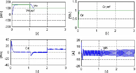
Fig. 3 illustrates the response speed of loadness machine, similar to a first-order system without being exceeded, with a response time of about 0.17s. There is, however, the rejection of disturbance which is applied to 2s later.

Perfect matching occurs when changing the reference speed. This

confirms proper choice of the coefficients tuning controller nonlinear

speed.

At the starting point (t=0), a peak torque electromagnetic at the

machine load is 35 Nm, whereas after 2 seconds torque load drops to 10

Nm. The response to this load change with a dynamic torque is almost

instantaneous, with a very low overrun and without oscillations.

The response of Rotor flux of induction machine in the 1

st

order

system occurs along its reference path, without being exceeded, the

response time being significantly smaller in the order of 0.09 seconds,

whereby perfect decoupling between the flux and torque is observed.

When there is no load , the stator current absorbed by the machine

shows an oscillation both at boot time and at speed change. Once loaded,

the machine absorbs a current quasi-sinusoidal and r.m.s on the torque

load.

At change of speed at 100 rad / s, the electromagnetic torque decreases reaching a negative value of -10N.m which corresponds to the system collapse.

Fig. 3 – Nonlinear control for an induction machine with a speed +156rad/s

(9)

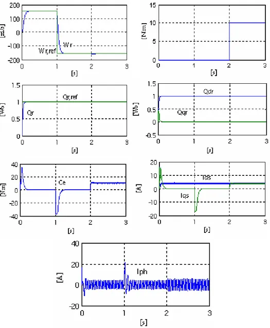
The reversal of rate of 156 rad s to –156 rad s at t=1s, according to Fig. 4, we note that the electromagnetic torque decreases instantly to a negative value of around –40Nm, which corresponds to an area of breaking and then switching to a rotation change.

Fig. 4 – Nonlinear control for an induction machine with a speed inversion

(10)

The flux does not have any influence due to the

perfect decoupling.

The simulation results show good performances for flux and the torque (speed), Fig. 4.

When the load torque is applied, we notice that there is no interaction between the two axes (d, q), which proves total dynamic decoupling between the two variables. The I_q current is proportional to the electromagnetic torque.

In addition, fluxΦ_ris oriented in the d direction (Φ = Φ Φ =_dr _r; _qr 0).

The speed responses are without static error, without overshooting and with a very fast disturbance rejection.

7 Conclusion

In this paper, we have presented the nonlinear control applied to the induction machine having rotoric flux orientation. The change of nonlinear co-ordinates and a negative feedback NL permits returning the nonlinear behavior of the system to linear system. The disturbances rejection and decoupling of flux and torque are acceptable.

The field-oriented control technique supposes that the knowledge of the flux position is exact. The nonlinear control makes abstraction of flux position. The nonlinear regulator retains the same performance

for a long time whereby we

are not acquainted with uncertainty parameters.

It is well adapted to the problems of tracking trajectories and the problems of stabilization. The main limitations are the lack of robustness and the practical point of view, the requirement that all states are measurable.

The main disadvantage of the

linearization order

is that it is based on the knowledge of the exact model of system. Indeed, in most cases we can not know the exact model of the real system

8 References

[1] B.K. Bose: Power Electronics and AC Drives, Printice Hall, New York, 1986.

[2] A. Isidori: Nonlinear Control Systems, Springer-Verlag, Berlin, 1989.

[3] B. Le Pioufle, G. Georgiou, I.P. Louis: Application of NL Control for the Speed or in

Position Regulation of the Autopilot Synchronous Machine, Physical Review Applied, 1990, pp. 517 – 527.

[4] B. Le Pioufle: Comparison of Speed Nonlinear Control Strategies for the Servomotor,

Electric Machines and Power Systems, Vol. 21, No. 2, Mar. 1993, pp. 151 – 169.

[5] B. Belabbes: Linearizing Control of a Synchronous Permanent Magnet Machine, Thesis of

Magister, University of Sidi Bel Abbès, 2001.

[6] R. Boukezzoula: Commande Floue d’une classe de système non linéaires: Application au

(11)

de Micro-Informatique Industrielle (LAMII/CESALP) de l’Ecole Supérieure d’Ingénieurs d’Annecy, Université de Savoie, 31 Mars 2000.

[7] H. Hamdaoui, A. Semmah, Y. Ramdani, M.K. Fellah: Fuzzy Learning Control of Advanced

Superconducting Magnetic Energy Storage to Improve Transient Power System Stability Node to End-user, Iranian Journal of Electrical and Engineering, Vol. 3, No.2, Summer-fall 2004, pp. 95 – 102.

[8] M. Fliess, I. Kupka: A Finitness Criterion for Non Linear Input-output Differential Systems,

SIAM Journal of Control and Optimization, Vol. 21, No. 5, 1983, pp. 721 – 728.

[9] A. Kadouri, S. Blais, M. Ghribi: Développement d’un outil de conception non linéaire basé

sur lagéométrie différentielle, Proceeding CEE’02, Batna, 10-11 Dec 2002, pp. 74 – 79.

[10] T.V. Raumer: Adaptative Nonlinear Control of the Asynchronous Machine, Thesis of

Doctorate, I.N.P of Grenoble, 1994.

[11] S. Hyungbo, H.S. Jin: Non-Linear Output Feedback Stabilization on ha Bounded Region of

Attraction, International Journal of Control, Vol. 73, No. 5, March 2000, pp. 416 – 426.

[12] A. Bentaallah, A. Meroufel, A. Massoum, M. K. Fellah: Control and Input-output

Linearization of an Asynchronous Machine, Conference on Electrotechnics ICEL 2005, U.S.T. Oran University, Algeria, November 13-14, 2005.

[13] A. Nekrouf: Commande non linéaire adaptative floue d’une machine asynchrone, Thèse de

magister en électrotechnique, Université de Sidi Bel Abbès, 2007.

[14] A. Bentaallah: Linéarisation Entré-sortie et réglage floue d’une machine asynchrone avec

pilotage vectoriel et observateur à mode glissant, Thèse de magister en électrotechnique, Université de Sidi Bel Abbès, 2005.

[15] M.K. Maaziz., E. Mendes, P. Boucher: Nonliear Multivariable Real Time Control Strategy of

Induction Machine Based on Reference Control and PI Controllers, 13th Int. Conf. on Electrical Machines ICEM’2000, Espoo, Finland, August 28-30, 2000.

[16] K. Theocharis, Boukas, and G. Thomas, Habetler: High Performance Induction Motor Speed

Control using Exact Feedback Linearization with State and State Derivative Feedback, IEEE. Trans. on Power Electronics, Vol. 19, No. 4, July 2004, pp. 1022 – 1028.

9 Induction Machine Parameters

2

1.5 kW 2

380 220 V, 50 Hz 1450 tr min

3 6 A 0.258 H

4.85 3.81

0.274 H 0.274 H

0.031Kgm 0.0114 Nm rad s

s r

P p

U N

I M

R R

L L

J f

= =

= Ω = Ω

= =