Weighted Twin Support Vector Machine with Universum

Weighted Twin Support Vector Machine with Universum

Shuxia Lu1,*_{, Le Tong}2

1

College of Mathematics and Computer Science, Hebei University Baoding, Hebei, 071002,China

cmclusx@126.com

2

College of Mathematics and Computer Science, Hebei University Baoding, Hebei, 071002,China

tonglmo@163.com

Abstract

Universum is a new concept proposed recently, which is defined to be the sample that does not belong to any classes concerned. Support Vector Machine with Universum (�-SVM) is a new algorithm, which can exploit Universum samples to improve the classification performance of SVM. In fact, samples in the different positions have different effects on the bound function. Then, we propose a weighted Twin Support Vector Machine with Universum (called �-WTSVM), where samples in the different positions are proposed to give different penalties. Therefore �-WTSVM has better flexibility of the algorithm and can obtain more reasonable classifier in most case. All experiments demonstrate that our �-WTSVM far outperforms TSVM, and lightly outperforms �-TSVM not only in linear case but also in nonlinear case.

Keywords: Universum, TSVM, �-SVM, Weight.

1. Introduction

SVM with Universum is a new method and the basic idea is to incorporate a priori knowledge into the learning process. The Universum sample concept has been introduced by Weston, Collobert, Sinz, Bottou, and Vapnik in 2006 [1]. The Universum is defined as a collection of unlabeled examples known not belong to any class. Then Weston et al., give a modified Support Vector Machine (SVM) [12] framework, called �-SVM [1] and their experiment results express that �-SVM outperforms those SVMs without considering Universum data. Sinz et al., gave an analysis of

�-SVM[2]. Examples from the universum are not belonging to any of the classes the learning task concerns, but they reflect a priori knowledge about application domain [1]. About the Universum data improvement can be found in [4] .Some extensions to the

�-SVM can be found in [3]-[7].

In order to improve the SVM computational speed, Jayadeva et al. [8] proposed a twin support vector

machine (TSVM) classifier for binary classification. TSVM generates two nonparallel hyper-planes by solving two small QPPs such that each hyperplane is closer to one class and is as far as possible from the other one [9]. Solving two smaller sized QPPs rather than a single large one, makes the learning speed of TSVM approximately four times faster than the standard SVM. Other literatures also can be found in [10] and [11].

In this paper, inspired by the success of [1] and [12], we proposed a weighted Twin Support Vector Machine with Universum (called �-WTSVM),give different penalties to the samples depending their different positions. This method not only retains the superior characteristics of

�-TSVM, but also has its additional advantages: comparable or better classification accuracy compared to

�-SVM, and TSVM. Moreover, the running time does not increase much.

The remaining parts of the paper are organized as follows. Section 2 briefly introduces the background of TSVM and �-SVM; Section 3 describe the detail of

�-WTSVM; All public datasets experiment results are shown in the section 4; In the last section gives the conclusions.

2. Background

In this section, we give a brief outline of TSVM[8] and

�-SVM[1]. For classification about the training set

= 1, 1 , 2, 2 ,… , , where ∈

and ∈ 1,−1 , = 1,…, .

2.1 TSVM

Consider a binary classification problem of 1 positive

points and 2 negative points. Suppose that the data

points in class +1 are denoted by ∈ 1× _{, where}

each row ∈ represents a data point. Similarly,

Linear TSVM searches for two nonparallel hyperplanes

1 = 1 + 1= 0

2 = 2 + 2= 0

(1)

where 1∈ , 2∈ , 1∈ and 2∈ . Such

that each hyperplane is proximal to the data points of one class and far from the other class.

The TSVM classifier is obtained by solving the following pair of QPPs

1,1, 1

2 1+ 1 1 1+ 1 1 + 1 2

. . − 1+ 2 1 + 2, 0, (2)

And

2,2,�

1

2 2+ 2 2 2+ 2 2

+ 2 1�

. . − 2+ 1 2 +� 1, � 0, (3)

where 1, 2 0 are parameters and 1, 2 are vectors

of one’s of appropriate dimensions. By introducing the Lagrangian multipliers, we obtain the Wolfe dual of TSVM as follows

₂ −1 2

−1

. . 0 1 (4)

and

1 −

1 2

−1

. . 0 2 (5)

Here, = 2 , = 1 , = 1 , and

= 2 , and the nonparallel proximal hyperplanes

are obtained from the solution and of (4) and (5) by

1=− −1 and 2 =− −1

Where 1= 1, 1 , 2= 2, 2 . The case of

nonlinear kernels is handled on lines similar to linear case.

2.2

�

-SVM

The basic theory of Universum SVM is based on the standard SVM method, by adding unlabeled samples in

the training process in order to get more information on the distribution of samples.

Let = 1, 1 ,… , be the set of labeled

examples and let = 1,…, denote the set of

Universum examples. A standard SVM using the hinge loss = 0, − can compactly be formulated as

,

1 2

2₊

, =1

(6)

the prior knowledge embedded in the Universum can be reflected in the sum of the losses =1 , ,

�-SVM use the ϵ-insensitive loss = ₋ +

− − for Universum

,

1 2 2

2₊

, =1

+ , =1

(7)

3. Weighted Twin Support Vector Machine

with Universum (

�

-WTSVM)

From the above description, we know that �-TSVM uses hinge loss function just as �-SVM, so this algorithm is less robust, in other words, sensitive to noises. This is the common drawback of any learning method using hinge loss function. In order to avoid this drawback, we consider weighted TSVM idea to improve the algorithm by using weights to modify error variables. The proposed algorithm is called weighted �-TSVM (�-WTSVM) by us.

3.1 Linear

�

-WTSVM

The formulations of Linear �-WTSVM are expressed as follows

1,1, , 1

2 1+ 1 1

2₊

1�1 + (8)

. .− 1+ 2 1 + 2, 0 (9)

₁+ ₁ + −1 + , 0 (10)

And

2,2,�, 1

2 2+ 2 2

2₊

2�2�+ (11)

− 2+ 2 + −1 + , 0 (13)

Where = ₁,…, , φ= ₁,…, and

, 1, 2, ∈ 0, +∞ are the prior parameters. The

Lagrangian based on the optimization problem (8)-(10) is given by

1, 1, , , , , , = 1

2 1+ 1 1

2₊

1�1 + − − 1+ 2 1 + − 2 −

− 1+ 1 + + 1− − (14)

where α,β, , are the members of the vectors of Lagrange multipliers. The Karush-Kuhn-Tucker (KKT) conditions for (14) are obtained as follows

1

= 1+ 1 1 + − = 0 (15)

1

= ₁ 1+ 1 1 + 2 − = 0 (16)

= ₁�₁− − = 0 (17)

= − − = 0 (18)

Since , 0, (17) and (18) turn to be

0 α 1�1 and 0

Combining (15) and (16) leads to

1 1 1 1 + 2

− = 0 (19)

Let = 1 , = 2 , 0 = , equation

(19) can be rewritten as

₁+ − = 0

i.e., 1=− −1 − . (20)

We can use (8)–(10) to solve the following convex QPP,

which is the Wolfe’s dual of �-WTSVM

, −

1

2 − −

1 _{− +}

2

+ � −1

s. t. 0 ₁�₁, 0 , (21)

Similarly, the dual of (11)–(13) is formulated as

, −

1

2 −

−1 _{− +}

1

+ � −1

s. t. 0 2�2, 0 , (22)

where = 2 , = 1 , = , the

augmented vector 1 1 is given by

2=− −1 − (23)

Once the augmented vectors of 1 and 2 are known,

the two separating planes are obtained. The class of an unknown data point is determined as

= argmin

=1,2 1

, _{2 (24)}

Where ₁ = ₁ + ₁ , ₂ = ₂ + ₂ ,

where | · | denotes the perpendicular distance of the point from the planes. Following the same idea, we extend

�-WTSVM to its nonlinear version.

3.2 Nonlinear Kernel Classifier

In order to extend our algorithm to nonlinear cases, we considering the following kernel-based surfaces instead of planes

, ₁+ ₁ = 0, , ₂+ ₂= 0 (25)

Where = and K is a chosen kernel function. Then the optimization problems of nonlinear �-WTSVM are constructed as follows

1,1, , 1

2 , 1+ 1 1

2₊

1�1

+

(26)

. . − , 1+ 2 1 + 2, 0

, ₁+ _{2 1} + −1 + , ψ 0

And

2,2,�, 1

2 , 2+ 2 2

2₊

2�2�

+

(27)

. . , 2+ 1 2 +� 1, � 0

− , 2+ 1 2 + −1 + , 0

The Wolfe dual of the problem (26) is formulated as follow

, −

1

2 �− � � �

−1

� − � + 2 + � −1

(28)

where _� = , 1 , � = , 2 ,

� = , , The augmented vector 1= 1 1 can be rewritten as

� ��1+ � − � = 0

i.e., 1= _{� �}

−1

� − � (29)

In a similar way, we can obtain the Wolfe’s dual of the optimization problem (27)

, −

1

2 �− � � � −1

� − � + 1 + � −1

(30)

. . 0 2�2, 0 ,

where _� = , 2 , � = , 1 ,

� = , , The augmented vector 2= 2 2 is given by

2=− � � −

1

� − � (31)

4. Experiments

To check the performances of the proposed �-WTSVM, we compare it with TSVM and �-TSVM on several datasets, including toy data and UCI datasets. In experiments, for each SVM algorithm for nonlinear kernels, a Gaussian kernel (i.e. , = � − −

1 2/2�2 )was selected. We implemented all

algorithms in MATLAB 2010 and carried out experiments on a PC with an Intel (R) Core 2 Duo processor (2.79 GHz), 4 GB of RAM. The parameters

1, 2, and the RBF kernel parameter σ are selected

from the set of values 2 =−7,…,7 by tuning a set comprising of random 10 percent of the sample set. In the experiments we set 1= 2= . Once the

parameters are determined, the tuning set is returned to the sample set to learn the final decision function.

4.1 Toy data

To give an intuitive performance of �-WTSVM in different numbers of Universum data, we firstly use a toy 2D data to test the influence of Universum data to the accuracy. The positive data and negative data are generated randomly from two Gaussian distributions. Universum data is also generated by Gaussian distribution. We use 200 positive data and 200 negative data as the data set, 40, 80, 160 unlabeled data as Universum samples respectively. For the experiment, we use the 20% of the points for training and others for testing. We select linear kernel for the toy dataset. The comparative results of TSVM, �-TSVM and �-WTSVM are shown in Fig 1. The second toy data is a nonlinear separated example, Fig 2 shows the results of TSVM,

�-TSVM and �-WTSVM.

From the Fig 1. It is easy to see that Universum data can indeed help our algorithm to seek more reasonable classifier. With the increase of the number of Universum data, the average accuracies of the three algorithms in the toy data are constantly being improved. Fig 2 shows that the knowledge embedded in the Universum points indeed helps the �-WTSVM to have better performance than its original model. From Fig 3, with the increase of Universum data, the average accuracies of the two algorithms are obviously improved, which means that Universum data can indeed help our algorithm to seek more reasonable classifier.

NU=40 NU=80 NU=160

(b)The result of �-WTSVM on the training set.

Figure 1: The performance comparison of �-TSVM and �-WTSVM on toy data. positive points(blue ‘o’), negative points(red ‘+’), Universum data(green ‘*’) , two nonparallel hyperplanes(blue solid line).

(a)The result of TSVM on the training set. (b)The result of�-TSVM on the training set. (c)The result of �-WTSVM on the training set.

(d)Two-dimensional projections of TSVM. (e) Two-dimensional projections of�-TSVM. (f) Two-dimensional projections of�-WTSVM.

Figure 2: The performance of TSVM, �-TSVM and �-WTSVM in the RBF case. positive points(blue ‘o’), negative points(red ‘+’), Universum

data(green ‘*’) , pink solid curves are the hyperplanes of TSVM, �-TSVM and �-WTSVM, respectively.

Figure 3: The accuracy rates of TSVM, �-TSVM and �-WTSVM in the

toy data.

4.2 UCI datasets

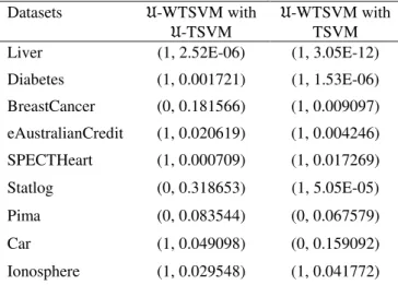
can find that the �-WTSVM which adds the Universum data outperforms the normal TSVM and �-TSVM in most cases. And then we use 10 times trials results of

�-WTSVM, �-TSVM and TSVM with t-test. The experimental results H and P show in Table 2. Compare with �-TSVM and TSVM, it is easy to find that the probability of �-WTSVM is extremely low,

this means that the accuracy of �-WTSVM are

significantly different with the other two.

Table 1:The testing accuracy and training times on UCI datasets in the case of RBF.

Datasets �-WTSVM accuracy

�-TSVM accuracy

TSVM accuracy time(s) time(s) time(s) Liver 80.00% 76.52% 67.83% (345×7) 0.1537 0.1944 — Diabetes 76.56% 75% 72.92% (768×9) 1.0162 1.0162 — BreastCancer 76.84% 76.32% 75.26% (569×31) 0.8255 0.9207 — AustralianCredit 68.26% 67.39% 66.52% (690×15) 1.3435 1.7382 — SPECTHeart 58.43% 56.18% 57.30% (569×31) 0.2896 0.3308 — Statlog 66.67% 65.22% 63.77% (690×15) 1.1039 1.6372 — Pima 82.81% 81.51% 81.25% (768×9) 0.4604 0.6470 — Car 70.72% 70.37% 71.41% (1728×7) 2.4714 2.6359 — Ionosphere 72.42% 70.44% 69.03% (351×34) 0.6344 0.6476 —

Table 2: The comparison results of �-WTSVM, �-TSVM and TSVM on t-test.

Datasets �-WTSVM with

�-TSVM

�-WTSVM with TSVM Liver (1, 2.52E-06) (1, 3.05E-12)

Diabetes (1, 0.001721) (1, 1.53E-06)

BreastCancer (0, 0.181566) (1, 0.009097)

eAustralianCredit (1, 0.020619) (1, 0.004246)

SPECTHeart (1, 0.000709) (1, 0.017269)

Statlog (0, 0.318653) (1, 5.05E-05)

Pima (0, 0.083544) (0, 0.067579)

Car (1, 0.049098) (0, 0.159092)

Ionosphere (1, 0.029548) (1, 0.041772)

5. Conclusion

Universum, which is defined as the sample that does not belong to either class of the classification problem of interest, has been proved to be helpful in supervised learning. In this paper, we have proposed a new weighted twin support vector machine with Universum algorithm (�-WTSVM) which is able to improve the classification performance.

Experimental results revealed that �-WTSVM is better than �-TSVM in terms of both classification effectiveness and lower computational cost. However, although

�-WTSVM performs faster than TSVM, the limitation is that it cannot handle large-scale problems. Thus, further work we will use the �-WTSVM to solve real large scale classification problems. And how to generate or select Universum data is also a main topic in the future.

Acknowledgments

Project supported by the National Nature Science Foundation of China (No. 61170040), by the Natural Science Foundation of Hebei Province (No. F2011201063, F2012201023).

References

[1] J. Weston, R. Collobert, F. Sinz, L. Bottou, V. Vapnik, "Inference with the Universum", ICML ’06μ Proceedings of the 23rd international conference on machine learning, ACM, 2006, pp. 1009–1016.

[2] F. H. Sinz, O. Chapelle, A. Agarwal, B. Scholkopf, "An analysis of inference with the universum", Advances in Neural Information Processing Systems 20, MIT Press, 2008, pp. 1369–1376.

[3] D. Zhang, J. Wang, F. Wang, C. Zhang, "Semi-supervised classification with universum", SIAM International Conference on Data Mining(SDM), 2008, pp. 323-333.

[4] S. Chen, C. Zhang, "Selecting informative universum sample for semisupervised learning". IJCAI, 2009, pp. 1016–1021.

[5] V. Cherkassky, S. Dhar, W. Dai, "Practical conditions for effectiveness of the universum learning", IEEE Transactions on Neural Networks , Vol. 22, No. 8 , 2011, pp. 1241–1255.

[6] C. Shen, P. Wang, F. Shen, H. Wang, "Uboost: Boosting with the universum", IEEE Transaction on Pattern Analysis and Machine Intelligence. Vol. 34, No. 4, 2012 , pp.825-832.

[7] Z.-Q. Qi, Y.-J. Tian, Y. Shi, "Twin support vector machine with Universum data", IEEE Transactions on Neural Networks , Vol. 36, 2012 , pp. 112–119.

[9] Y.-H. Shao, C.-H. Zhang, X.-B. Wang, N.-Y. Deng, "Improvements on twin support vector machines", IEEE Transactions on Neural Networks, Vol. 22, No. 6, 2011, pp. 962–968.

[10] M. A. Kumar, M. Gopal, "Application of smoothing technique on twin support vector machines", Pattern Recognition Letters, Vol. 29, No. 13, 2008, pp. 1842–1848.

[11] R. Khemchandani, Jayadeva, S. Chandra, "Optimal kernel selection in twin support vector machines", Optimization Letters, Vol. 3, No. 1, 2009, pp. 77– 88.

[12] N. Deng, Y. Tian, Support vector machines: Theory, Algorithms and Extensions, Science Press, China, 2009.

Shuxia Lu Professor of the Faculty of Mathematics and

Computer Science, Hebei University. Received the B.Sc. and M.Sc. degrees in Mathematics from Hebei University, Baoding, China, in 1988 and 1991, respectively, and the Ph.D. degree from Hebei University, Baoding, China, in 2007. Her main research interests include machine learning and computational intelligence, SVMs.

Le Tong Received the B.Sc. degree in Mathematics and its