Specific Land Cover Class Mapping by
Semi-Supervised Weighted Support Vector Machines
Joel Silva1,*, Fernando Bacao1and Mario Caetano1,2
1 NOVA Information Management School, Universidade Nova de Lisboa, Lisboa 1070, Portugal; [email protected] (F.B.); [email protected] (M.C.)
2 Direção Geral do Território, Lisboa 1070, Portugal
* Correspondence: [email protected]; Tel.: +351-213-828-610
Academic Editors: Chandra Giri, Parth Sarathi Roy, Richard Gloaguen and Prasad S. Thenkabail Received: 21 November 2016; Accepted: 15 February 2017; Published: 21 February 2017
Abstract:In many remote sensing projects on land cover mapping, the interest is often in a sub-set of classes presented in the study area. Conventional multi-class classification may lead to a considerable training effort and to the underestimation of the classes of interest. On the other hand, one-class classifiers require much less training, but may overestimate the real extension of the class of interest. This paper illustrates the combined use of cost-sensitive and semi-supervised learning to overcome these difficulties. This method utilises a manually-collected set of pixels of the class of interest and a random sample of pixels, keeping the training effort low. Each data point is then weighted according to its distance to its near positive data point to inform the learning algorithm. The proposed approach was compared with a conventional multi-class classifier, a one-class classifier, and a semi-supervised classifier in the discrimination of high-mangrove in Saloum estuary, Senegal, from Landsat imagery. The derived classification accuracies were high: 93.90% for the multi-class supervised classifier, 90.75% for the semi-supervised classifier, 88.75% for the one-class classifier, and 93.75% for the proposed method. The results show that accuracy achieved with the proposed method is statistically non-inferior to that achieved with standard binary classification, requiring however much less training effort.
Keywords:one-class support vector machines; weighted support vector machine; random training set; specific class mapping; land cover; mangrove; Landsat
1. Introduction
Today, remote sensing is an integral part of many research activities related to Earth monitoring [1]. In particular, supervised classification of remotely sensed data has become a fundamental tool for the derivation of land cover maps [2]. Indeed, users are often not interested in a complete characterisation of the landscape, but rather on a sub-set of the classes that occur in the region to be mapped. For example, users may be focused on mapping urban classes [3–5], abandoned agriculture [6], specific tree species [7,8], invasive wetland species [9], or mangrove ecosystems [10,11]. Fundamentally, depending on the application, the accurate discrimination of some classes is more important than the discrimination of others [12].
When interest is focused on a single class, the use of a conventional supervised classification process may be inappropriate [13]. Indeed, this approach assumes that the set of classes has been exhaustively defined [14,15]. Thus, the correct application of this analysis requires that all classes that occur in the study area be included in the training set [16,17]. Therefore, when mapping a region for a user interested in urban land cover, it will be necessary to collect training data points not only on the urban classes of interest, but also on secondary classes with no interest to the user, such as crops, forest, and water, if these are present in the area of study. If these classes are not included in the training data
set, the classifier will commit pixels of untrained classes into trained classes. For example, if the land cover class forest was not incorporated in the training data set, pixels of forest my be systematically classified as a type of shrub or crop, which greatly overestimates the real extent of those shrubs and crops classes. The user must therefore seek to ensure that all classes occurring in the region of interest are sampled to fulfil this requirement. In other words, the users have to allocate time and effort in training classes that are of no interest for their goals.
In addition, conventional supervised classification algorithms often are not optimised for the discrimination of a particular class [12,13]. The classification algorithm seeks a classifier where the overall classification accuracy—measured over all classes—is maximum [18]. The class of interest—which is typically just one and often a small part of the set of classes—may be neglected in the process, and thus the resulted model may not be optimised for the discrimination of that particular class and may underestimate the class of interest [19]. In other words, the classifier may accurately discriminate secondary classes to the detriment of the class of interest [13,16]. Hence, in both training and allocation stages, conventional supervised classification approaches are not focused on the class of interest. This places users’ wastefully directed training effort on classes of no interest and leads to an analysis that may not be optimal in terms of the discrimination of the important class. Therefore, when there is a particular class of interest, it may be preferable to follow an alternative approach to the conventional multi-class supervised classification method [20].
Literature shows that there are essentially two alternatives to the standard multi-class supervised approach: the binarisation strategy and one-class learning algorithms [21–23]. With binarisation strategy, users decompose the multi-class problem in a series of small binary classification problems where one seeks to separate the classes of interest from all irrelevant classes [22,24–26]. As binary classification is well-studied, binary decomposition of multi-class classification problems have attracted significant attention in machine learning research, and has been shown to perform well in most multi-class problems [24]. Indeed, binary decomposition has been widely used to develop multi-class support vector machine (SVM) showing better generalisation ability than other multi-class approaches [27]. The possibility to parallelise the training and testing of the component binary classifiers is also a big advantage in favour of binarisation, apart from their good performance [22]. In particular, binarisation can be achieved by combining all land cover classes of no interest into a large nominal class, called, for example, ”others” [28]. In this way, the class of interest can be regarded as the positive class and all others as the negative class in the binary classification scenario. Previous studies [8,10,26,28] have shown it to be possible to decompose the multi-class classification problem into a series of small binary classification problems and achieve results that are more suitable for the particular users’ requests; namely, the improvement of the discrimination of particular land cover classes of interest. Although specific class mapping can potentially be a better approach compared to the multi-class supervised classification, it has some particular difficulties, such as data imbalance in the training set [19,29]. This is because the classes of interest are often only on a small component of the study area [12], and the errors in classes that are not of importance are considered in the final overall accuracy [30,31]. In fact, directly applying a binary decomposition to the classification problem may result in a highly unproportional allocation of training points to the negative class, leading to imbalance in the training data set [29]. In addition, the binarisation approach also requires the users to collect training on classes of no interest, similarly to what happens in the multi-class approach.
able to bind the class distribution, the classifier may lead to over-expanded decision boundaries [23]. However, that deviation can only be assessed with training points outside of the class of interest [23]. Literature also shows that when information about the classification space outside the class of interest is available, binary classifiers tend to develop more accurate classifiers then the one-class approach [21,33].
In the specific class mapping context, since the class of interest is typically only a small component of the study site [12], the number of negative pixels are much larger compared to the number of positive pixels (i.e., the pixels of interest). Thus, there is typically an over-abundance of negative pixels such that the probability of an arbitrary unlabelled pixel to be negative is much higher than the probability of it being positive. In this context, the use of randomly selected data points can be an option to improve specific class mapping. This approach is typically known as semi- supervised learning.
Semi-supervised learning—also known as positive and unlabelled learning—refers to the use of unlabelled data points to inform the learning algorithm [34]. Here, semi-supervised learning can be a possible approach to the classification process, since a priori there is bias toward the negative class [35].
Previous works have used semi-supervised learning approaches to map land cover classes (e.g., [19,36]). In these studies, the biased support vector machine (BSVM) algorithm has been utilised with success to map classes like urban and tree tops from aerial imagery [37], and to classify single tropical species [19]. With BSVM, the unlabelled set is regarded as the negative class, and the cost associated to the positive class and the negative class are asymmetrical, so that an error occurring in the positive class is costlier than an error on the negative (unlabelled) class [38]. However, it is not clear how to set up the weights, and the trial-and-error approach usually takes a long computation time [39].
A similar approach is presented in this paper; however, a different cost-sensitive approach is employed. A set of randomly defined unlabelled data points is used as an approximation to the negative class, and only the positive class (the class of interest) is manually sampled. However, the costs associated to each class are not asymmetrically defined; rather, the individual data points are weighted differently according to their similitude to a positive data point. This similitude metric is a function of the euclidian distance to its nearest positive data point. The heuristics followed here is that the likelihood of a negative data point to be mislabelled depends on its proximity to a known positive data point. Note that the positive data points are manually defined by an human analyst, and thus considered certain and correct. The weight distribution in the negative class is then used by a cost-sensitive learning algorithm to develop a binary classifier. In other words, the proposed method aims to develop a binary classifier to classify a particular class of interest with the same sampling effort that is required by the one-class classifiers, but providing the same discriminating information of a binary classification. Here the proposed method was compared with three different alternative approaches: First, the conventional multi-class supervised approach—here, an SVM classifier. This method was selected because it is today a staple analytical tool of many remote sensing data analysts [2], implemented in the majority of remote sensing software and data analysis programming languages (e.g., R). Second, a single-class classifier, the OCVM. Third, a semi-supervised method: BSVM. These two methods (BSVM and OCSVM) were selected because they have been previously used in a variety of studies with remotely-sensed data, such as [13,17,19,37,40].
2. Background
The SVM algorithm is a popular supervised classification algorithm that has been successfully applied in many domains [20]. In particular, the study and application of SVM is extensive and well known in the classification of remotely sensed imagery [2]. Most implementations of SVM require the solution of the following optimisation problem [41]:
min w,ξ
1 2w
subject toyi(wTφ(xi) +b)≥1−ξifori=1 . . .m, wheremis the number of training data points,wis the hyperplane normal vector,φis the kernel function,eis the all 1’s vector, andξis the vector of slack variables. The parameterCrepresents the magnitude of penalisation. IfCis a large value, the optimal solution defines narrower margins in order to accommodate the misclassified training data points; in contrast, smaller values ofClead to wider margins [42]. The penalisation strategy here is uniform, and thus equally applied regardless of the class and the data point being analysed.
This is not limited to SVM. Indeed, in conventional supervised classification methods, the aim is to minimise the general misclassification rate, and thus all types of misclassification are regarded as equally severe [18]. A more general approach is to consider misclassifications as not equal. That is, some errors are regarded as more costly than others. This difference is then utilised to inform the learning algorithm during the classification induction stage, and drive the induction process more sensitively. There are essentially two ways to implement a cost-sensitive approach: the class-dependent and the instance-dependent. However, which approach is the more suitable dependents of the problem at hand. Next are presented two implementations of these approaches: the BSVM, implementing of the class-dependent cost definition; and weighted SVM (WSVM), implementing the instance-dependent.
2.1. Bias SVM and Weighted SVM
The BSVM is an adaption of the classical formulation of the SVM to handle unlabelled data [38]. This is done by defining different cost values to the positive and to the negative (unlabelled) classes.
min w,ξ
1 2w
Tw+CpeTξ
p+CneTξn, (2)
subject toyi(wTφ(xi) +b)≥1−ξifori=1 . . .m. The vectorξpis the vector of slack variables of the positive data points, andξnis the vector of slack variables of the negative data points. The parameters CpandCnrepresent the penalisation cost of misclassifications in the positive and negative classes, respectively. Thus, by varyingCpandCn, it is possible to penalise the positive class and the negative class differently. Intuitively, the cost values are assigned such thatCpis a large value compared to Cnbecause the positive class was defined by an human analyst (and thus assumed correct), and the negative class is originated from a random sample of pixels, and thus possibly containing positive data points [36]. However, there is no clear indication of how to define those parameters, and trail-and-error is generally recommended [38].
Differently from the SVM and BSVM, the WSVM implements an instance-dependent cost scheme; that is, instead of penalising classes (like with the BSVM) or all data points equally (like with the SVM), the goal is to penalise individual data points. A way to adapt the SVM approach to inform the optimisation problem that some points are more relevant than others is by incorporating a weight vector that assigns different cost values to different data points [43,44]. The original SVM problem is thus reformulated in the following way:
min w,ξ
1 2w
Tw+CσTξ, (3)
subject toyi(wTφ(xi) +b) ≥1−ξi fori = 1 . . .m, whereσ is the vector of weights. The user can then set different weights to different data points according to a predetermined criterion. Applying the Karush–Kuhn–Tucker conditions, the original WSVM problem can be reformulated in its dual form [44]:
min
α
1
2.2. One-Class SVM
In its origin, the SVM was developed to solve binary classification problems with linearly separable classes. However, the same principles can be applied to solve one-class problems—also known as novelty detection problems [45]—that consist of detecting objects from a particular class. This class is often called “target class” or “class of interest”. These problems differ greatly from the standard supervised classification in the sense that the training set is composed exclusively of data points from the target class, and thus there are no counterexamples to define the classification space outside the class of interest. One-class classification has been utilised in a variety of applications [46], and has great potential in remotely-sensed data processing. There are two approaches to one-class classification based on SVM principles: the OCSVM [45] and the support vector data description (SVDD) [47]. In this paper, focus is on the use of OCSVM.
The idea behind the OCSVM is to determine a function that signals positive if the given data point belongs to the target class, and negative otherwise. To achieve that, the classification space origin is treated as the only available member of the non-target class. The problem is then solved by finding a hyperplane with maximum margin separation from the origin. Non-linear problems are dealt with a kernel function as in the binary SVM. The OCSVM optimisation problem is formulated as follows [45]:
minw,ξ,ρ 1 2w
Tw
−ρ+ 1
νm
∑
i ξi, (5)subject towTφ(xi)≥ρ−ξiandξi≥0. Here,mis the number of training data points,wis the vector perpendicular to the hyperplane that defines the target class boundaries, andρis the distance to the origin. The functionφis related with the kernel function [45]. The use of slack variablesξiused in the OCSVM allow the presence of class outliers, similar to binary SVM. The parameterνranges from 0 to 1, and controls the trade-off between the number of data points of the training set labelled as positive by the OCSVM decision functionf(x) =sign(wTφ(x)−ρ).
2.3. Free-Parameter Tuning
The development of a learning algorithm requires the use of accuracy metrics to assess the quality and compare the performance of alternative classifiers. In particular, the determination of these free-parameters is an important step. Indeed, there is empirical evidence suggesting that parameter tuning is often more important than the choice of algorithm [48]—SVM being particularly harder to tune than other classification procedures [49].
The determination of the best values of the learning algorithm parameters is typically done by cross-validation trials [50,51]. The range of the parameters is divided in a grid, and the training set is broken into parts (e.g., five). Each part is in turn used as testing set, and all others are used as training set. Then, a classifier is induced using the training set and tested with the testing set. The classification errors yielded with each part are then averaged, and the parameterisation with the least classification error is selected [52]. Although there are studies developing methods to determine these parameters (e.g., [53,54]), the cross-validation method is still the method adopted by the majority of data analysts [51,52].
data set is imbalanced and the classification accuracy is utilised, the outcome of the tuning process will indicate that a particular parameterisation is the one with the highest classification accuracy. However, it may be biased towards the majority class, since that parameterisation may yield a classifier that very accurately classifies the majority class to the detriment of the minority class [43]. Since the class of interest is often just a small component of the training, the classifier would then underestimate the true extension of this small but important class.
There are better alternative accuracy metrics to the classification accuracy; for example, sensitivity and specificity [50]. Sensitivity is the proportion of true positives correctly classified, while specificity is the proportion of true negatives correctly classified [44]. In this way, sensitivity indicates how good the classifier is at recognising positive cases, and specificity indicates how good the classifier is recognising negative cases [44]. Note that in binary classification, classification accuracy may not be a reliable indicator—particularly if the data set is imbalanced, since the influence of the majority class is much higher than that of the minority class [43].
Sensitivity and specificity are often combined in one metric for better analysis and comparison [57]. In particular, the geometric mean between sensitivity (s) and specificity (S) [18,58], Equation (6), is particularly useful:
G=√sS (6)
The geometric mean (G) indicates the balance between classification performances on the positive and negative classes. A high misclassification rate in the positive class will lead to a low geometric mean value, even if all negative data points are correctly classified [43]; a similar result is obtained if the classifiers show high misclassification in the negative class. In this way, if both sensitivity and specificity are high, the geometric meanGis also a high value; however, if one of the component accuracies—sensitivity or specificity—is low, the geometric meanGis affected by it. Thus, a classifier with high geometric mean is highly desirable for class-specific mapping [59], and henceGcan be used to fine-tune binary algorithms of classification.
A particular observation is necessary for BSVM. Since the positive class and the negative class are penalised differently, the BSVM effectively has two penalisation variables, which complicates the grid-search optimisation process. In general, the penalisation cost of the positive class should have a large value compared with that of the negative class, because it is unknown whether the unlabelled samples are actually positive or negatives. However, there is no clear criterion to adjust these parameters, and often the user has to resort to trial-and-error [38].
Like SVM, the OCSVM algorithm depends on free-parameters that need to be set to develop the classifier. These free-parameters consist of kernel parameters (e.g., the radial factor of the radial-basis kernel function and the degree of the polynomial kernel), and regularisation parameters. In the case of OCSVM, the regularisation parameter isν, ranging from 0 to 1, and defines the upper bound of the fraction of training data points regarded as outliers and and the lower bound of the fraction of training data points regarded as support vectors [45]. In binary and multi-class classification, the determination of the free-parameters is often done by grid-search cross-validation using the classification accuracy as metric [29,52]. However, the training set used with these types of classifiers does not contain data points outside the class of interest, and thus it is only possible to assess the sensitivity of the classifier in the cross-validation process [36,37]. Using only the sensitivity to parameterise a classification algorithm may result in a classifier with high sensitivity but low specificity, overestimating the true extension of the class of interest.
ˆ
θ=argmaxθ
1
n∑kI(fθ(xk) = +1) Nsv(fθ)
. (7)
function parametrised withθ, andNsvis the number of support vectors in fθ. This ratio enforces high
sensibility while limiting model complexity (the number of support vectors), which usually indicates good model generalisation ability [60].
3. Methods
3.1. Study Area
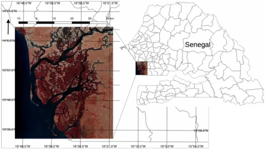
The study area is located in Saloum river delta in Senegal, Africa (Figure 1). The area is predominantly flat, with altitudes ranging from below sea level in the estuarine zone to about 40 m above mean sea level inland. The climate is Sudano-Sahelian type with a long dry season from November to June and a 4-month rainy season from July to October [61,62].
Figure 1.Saloum river delta in Senegal.
The regional annual precipitation—which is the main source of freshwater recharge to the superficial aquifer—increases southward from 600 to 1000 mm. The hydrologic system of the region is dominated by the river Saloum, its two tributaries (Bandiala and Diomboss), and numerous small streams locally called “bolons”. Downstream, it forms a large low-lying estuary bearing tidal wetlands, a mangrove ecosystem, and vast areas of denuded saline soils locally called “tan” [62]. The largest land cover classes present in the study area are water, mangrove species, shrubs, savannah, and bare soil. The main crop is millet, and the urban settlements are usually small and sparse. Saltpans develop to the north because of excessive salinity [63]. In this paper, interest is focused on one type of mangrove: high-mangrove. High-mangrove is generally characterised by a dense and tall canopy, and is composed of species likeRhizophora racemose,Rhizophora mangle, andAvicennia Africana[64]. The mapping of this particular land cover class is important for the monitoring and preservation of the Saloum river delta, as its presence or absence is closely related to the mangrove system health [62,64]. The Saloum river delta was designated a UNESCO World Heritage site for its remarkable natural environment and extensive biodiversity, and is listed in the Ramsar List of Wetlands of International Importance [63]. Particularly important is Saloum’s mangrove system, occupying roughly 180,000 ha supporting a wide variety of fauna and flora, and the local economy [63].
3.2. Remotely Sensed Data and Training Set
and the atmosphere may be considered to be homogeneous within the study area, atmospheric correction was not necessary [65]. The digital numbers were normalised using the max–min rule to range from 0 to 1.
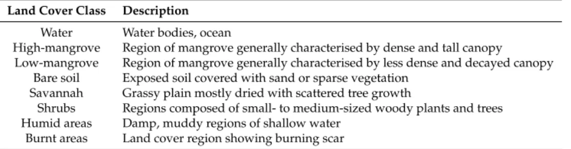
The study area is mostly composed of eight large land cover classes (Table 1): water, high-mangrove, low-mangrove, bare soil, savannah, shrubs, humid areas, and burnt areas. The training set is comprised of 100 pixels per class for each of the eight land cover classes.
Table 1.Land cover classes composing the study area and their description.
Land Cover Class Description
Water Water bodies, ocean
High-mangrove Region of mangrove generally characterised by dense and tall canopy Low-mangrove Region of mangrove generally characterised by less dense and decayed canopy
Bare soil Exposed soil covered with sand or sparse vegetation Savannah Grassy plain mostly dried with scattered tree growth
Shrubs Regions composed of small- to medium-sized woody plants and trees Humid areas Damp, muddy regions of shallow water
Burnt areas Land cover region showing burning scar
3.3. Experiments
Four experiments were conducted where the first two experiments were used as benchmark. In the first, an OCSVM classifier was developed using only training data of the class of interest (high-mangrove). This experiment is thus labeled as OCSVM. The kernel function utilised in the analysis was the radial-basis function, and its free-parameters were fine-tuned using 10-fold cross-validation, as described in Section2.3. From this analysis, the free-parameters were set as γ=0.0000610 andν=0.025.
In the second experiment, an image analyst collected 100 points per land cover present in the study area, comprising a total of 800 data points. The data points labeled as high-mangrove were reclassified as positive (class of interest), and the remain training points were reclassified as negative (class of no interest). Next, an SVM was developed to discriminate exclusively the class of interest. This experiment is labeled as SVM. The kernel function utilised for analysis was the radial-basis, and its free-parameters were set with 10-fold cross-validation asγ=2 andC=0.125, using the geometric mean as described in Section2.3. This approach consists of a common binarisation process of the classification problem, and has been successfully used in previous studies (e.g., [26]), and extensively studied by machine learning researchers (e.g., [22,24,25]).
The third and fourth experiments were conducted in a semi-supervised way. Thus, a simple random sample of pixels was utilised to collect random pixels throughout the study scene, composed of 1000 pixels. Following the semi-supervised approach, these were then labelled as negative without individual verification [34,37]. Next, only the class of interest was sampled by an analyst, similar to what happened with the one-class approach. In the third experiment, a BSVM classifier was trained. The kernel function utilised for analysis was the radial-basis, and its parameters (γ,Cp, andCn) were set by trial-and-error ensuringCn < Cp, since negative class may contain mislabelled data points.
From this analysis,γ=2,Cp=256, andCn=0.03125.
considered certain, and thus correct. Negative points, however, which were randomly selected and blindly labelled as negative, may be misclassified. The number of negative training data points that are mislabelled is expected to be small, since the area occupied by the class of interest is also expected to be small (roughly 10% from previous studies; e.g., [62]).
The function utilised to relate the spectral distance with the nearest positive point was the exponential function in Equation (8):
wi=1−exp(−σd2i), (8)
wherewiis the weight of theith random point andd2i is the squared euclidean distance of theith random point to its nearest positive point in the feature space. The free-parameterσ>0 is utilised as
a smoothing parameter; large values ofσincrease the average weight of the points, while small values reduce it. Note that the maximum assigned weight is 1, and the smallest is asymptotically 0. Thus, the misclassification of data points with large weights (close to 1) are more costly that the misclassification of points with less weight (close to 0). In this way, the learning process is informed of which training points are more important to define the decision boundaries. Since it is necessary to assign a weight value to all training data points, the positive points were assigned the maximum weight 1, because these are considered certain and correctly labeled.
Note that this weighting model is not necessarily unique. Indeed, any function assigning distances to the interval of 0 to 1 may be used. However, the exponential function is sufficiently sophisticated to represent the intuitive behaviour of decay, but simple enough to produce results with a minimum of data [66].
Nevertheless, the purpose of this study is not to determine which weight-assigning functions are the most suitable under given conditions, but rather to show the general effectiveness of the method. Thus, only the exponential function was utilised.
Similar to the SVM, the kernel function that was used was the radial-basis function, and its free-parameters were defined using a 10-fold cross-validation process with the geometric mean as metric. From this analysis, these were set asγ = 2 andC = 512. The values of σ were set by trial-and-error. A range of values were tested ranging from very small (0.01) to large (10); at the end, the best value forσwas 1. All weight values were then normalised using the maximum weight. From this analysis, the weights of the negative data points ranged from 0.001 to 0.86.
All experiments where conducted with LibSVM version 3.21 and LibSVM-weights version 3.20.
3.4. Classification Accuracy and Comparison
Classification accuracy was estimated using an independent testing set of 2000 simple random pixels, as it is not practical to ground truth in every pixel of the classified image [5]. An image analyst visually classified each pixel, labelling the point as positive (belonging to high-mangrove) or negative (not belonging to high-mangrove) in the same month and year (February 2015) as the image acquisition, with support of Google Earth and Google Maps. From this analysis, 107 pixels were labeled as positive and 1893 were labeled as negative. The accuracy of each classification was expressed in terms of the proportion of correctly classified testing data points, and also using sensitivity and specificity. Sensitivity is the proportion of positive pixels correctly classified, while specificity is the proportion of negative pixels correctly classified [29]. More concretely, the classification accuracy (a) is obtained by
a= n
N, (9)
sensitivity (s) is determined using
s= n+
N+, (10)
S= n−
N−, (11)
wherenis the number of testing points correctly classified, andNis the total number of testing points. n+is the number of positive cases correctly classified, andN+the total number of positive cases in
the testing sample. Similarly,n−is the number of negative cases correctly classified andN−the total number of negative cases in the testing sample.
Since a single testing set was used for each test site, the statistical significance of the difference in overall accuracy between different classification approaches will be assessed using the McNemar test [67]. The McNemar test is based on a binary contingency table in which pixels are classified as correctly or incorrectly allocated by the two classifiers under comparison. The main diagonal of this table shows the number of pixels on which both classifiers were correct and on which both classifiers were incorrect. The McNemar test, however, focuses on the proportion of pixels where one classifier was correct but the other was incorrect. The analysis will be based upon the evaluation of the 100(1−α)% confidence interval, whereαis the level of significance, for the difference between two accuracy values expressed as proportions (e.g.,p1andp2) expressed as [68]:
p2−p1±zαSE, (12)
where the termSEis the standard error derived of the difference between the proportions, which can be determined by [68]:
SE=
r
p01+p10−(p01−p10)2
n (13)
wherep10the proportion of testing pixels where the first classifier was correct and the second was
incorrect, andp01the proportion of testing pixels where the first classifier was incorrect and the second
was correct. In this way, the statistical assessment of the differences was conducted to determine if these were significantly different or not [67]. To perform this analysis, it is necessary to define the zone of indifference [67]. This is the largest amount of allowable difference that determines if the methods are considered equivalent or non-inferior [69]. In this evaluation, it was assumed that the zone of indifference was 1.00%. Although this value was selected arbitrarily, it ensures that small differences in accuracy are inconsequential [70].
4. Results
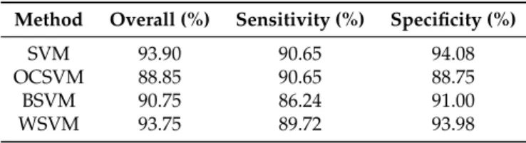
Table2summarises the accuracy metrics, overall accuracy, sensitivity, and specificity obtained with each method in the discrimination of high-mangrove land cover class.
Table 2.Overall accuracy, sensitivity, and specificity for each method. Results are in percentage. SVM: support vector machine; OCSVM: one-class SVM; BSVM: biased SVM; WSVM: weighted SVM.
Method Overall (%) Sensitivity (%) Specificity (%)
SVM 93.90 90.65 94.08
OCSVM 88.85 90.65 88.75
BSVM 90.75 86.24 91.00
WSVM 93.75 89.72 93.98
values were high, ranging from a maximum of 94.08% (93.10%, 94.90%) with SVM to a minimum of 88.75% (87.55%, 89.95%) achieved by OCSVM; BSVM achieved 91.00% (89.91%, 92.09%) and WSVM 93.98% (93.08%, 94.88%).
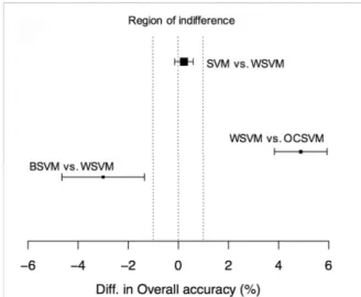
Figure2summarises the statistical comparison between the classifications.
Figure 2.The overall accuracies of each method and their respective 95% confidence interval.
The difference between the classification accuracies yielded by SVM and WSVM was 0.15% ranging from−0.09% to 0.39% at 95% confidence interval. On the other hand, the difference between the classification accuracies yielded by WSVM and OCSVM was 4.90% ranging from 3.85% to 5.95% at 95% confidence interval. Finally, the difference between the classification accuracies yielded by BSVM and WSVM was−3.00%, ranging from−4.55% to−1.35% at 95% confidence interval.
5. Discussion
The confidence interval for the difference (Figure2) in accuracy is within the region of indifference (−1%, 1%), and thus provides evidence for the non-inferiority of WSVM. In other words, the statistical analysis shows that the classification accuracy derived from WSVM is non-inferior to that of SVM at the 5% level of significance. However, WSVM was developed without the need to collect training data points in secondary classes, which contrasts with SVM, where all classes present in the study area were incorporated in the training set. Indeed, the sampling effort was similar to that of OCSVM, but the confidence interval is outside and above the region of indifference without intersecting it. This provides evidence for the difference between the classifications at the 5% significance level.
Comparing the two semi-supervised classification methods (BSVM and WSVM), the confidence interval is outside and below the region of indifference without intersecting it. However, the difference is smaller than that with OCSVM. Note that if the region of indifference were increased to (−2%, 2%), the conclusion would not change, since the interval defining the difference between BSVM and WSVM would not cross zero, although there would be an overlapping region. The main difference between BSVM and WSVM is in the way the learning algorithms deal with the negative class. BSVM penalises all points of the negative class in the same amount. The WSVM, on the other hand, particularises the penalisation. This leads WSVM to trust some negative training data points in the same way as a positive training data point and disregard some negative points as blunders.
of interest in the classification space, leading to more pixels to be allocated to the class of interest, particularly those close to the boundary of the class of interest.
Sensitivity values were also high. In particular, 90.65% for SVM and OCSVM, 86.24% for BSVM, and 89.72% for WSVM. The high value yielded by OCSVM can be explained by the over-extension of the decision boundary, which is extended enough to accommodate a large number of positive testing data points. The lower value yielded by WSVM and BSVM, when compared to SVM, can be a consequence of the way the negative data set was sampled. With the training set used by SVM, all classes present in the study site were sample.
Thus, the classification space outside the class of interest (the negative class) is well characterised in the sense that it contains samples describing all spectral patterns present in the image [71]. In other words, all regions of the negative classification space are represented in the training set. That may not happen with the WSVM and BSVM, where the training data was randomly generated. In other words, some regions of the classification space may not have been sample, and thus the resulted classifier may be committing untrained areas to the class of interest. Indeed, WSVM and BSVM errors occur mostly in forest and shrub class in areas spectrally similar to the class of interest—high-mangrove.
Figure3shows four excerpts of the maps produced by each method, where frame (a) is the WSVM map, (b) the OCSVM map, (c) the SVM map, and (d) the BSVM map.
Figure 3.Excerpts of (a) the WSVM map, (b) the OCSVM map, (c) the SVM map, and (d) the BSVM map. Top-left corner (332427,1536155) bottom-right (343366,1529391) EPSG: 32628.
results (Table2), where BSVM is the least sensitive method. Frame (a) and frame (c) indicate that the WSVM and SVM induced similar classifications, as also supported by the statistical analysis (Figure2). Note that the purpose of this analysis is not to provide support for the claim that the WSVM yields significant accuracy improvements over the SVM, but rather to support that WSVM yields results not inferior to those of SVM requiring much less training effort than the SVM. Indeed, with WSVM, the user needs only to manually sample the class of interest, like with the OCSVM.
6. Conclusions
This paper proposes and tests a method that aims to reduce the training sampling effort in class-specific mapping. The motivation for the development of this method comes from the fact that although one-class classification requires the user to collect only training data from the class of interest (which represents a great reduction in training effort), these methods may overestimate the class of interest. Typically, if information about the class of interest and the classes of no interest is available, binary classifiers tend to achieve higher classification accuracy. However, these methods require the user to collect training data from classes of no interest. The proposed method combines the sampling effort required by the one-class classifier with the discrimination capability of a binary class using a semi-supervised approach with cost-sensitive learning. The results indicate that although the four methods under analysis achieved high overall classification accuracy, the one-class classification achieved the lowest classification accuracy (88.85%) due to the overestimation of the extension of the class of interest, and the proposed method (93.75%) was non-inferior to the binary classification (93.90%) at the 5% level of significance, requiring however less training effort.
Acknowledgments: Research by Joel Silva was founded by the “Fundação para a Ciência e Tecnologia” (SFRH/BD/84444/2012) and was used in partial fulfilment of Joel Silva’s doctoral dissertation. The authors would like to thank the four anonymous reviewers for their contributions which have greatly improved the original manuscript.
Author Contributions:Joel Silva processed the data and wrote the paper. Fernando Bacao and Mario Caetano helped improving the manuscript. All authors contributed in the development of the idea.
Conflicts of Interest:The authors declare no conflict of interest.
References
1. Corbane, C.; Lang, S.; Pipkins, K.; Alleaume, S.; Deshayes, M.; Garcia Millan, V.E.; Strasser, T.; Vanden Borre, J.; Toon, S.; Michael, F. Remote sensing for mapping natural habitats and their conservation status—New opportunities and challenges.Int. J. Appl. Earth Obs. Geoinf.2015,37, 7–16.
2. Mountrakis, G.; Im, J.; Ogole, C. Support vector machines in remote sensing: A review. ISPRS J. Photogramm. Remote Sens.2011,66, 247–259.
3. Feng, X.; Foody, G.; Aplin, P.; Gosling, S.N. Enhancing the spatial resolution of satellite-derived land surface temperature mapping for urban areas. Sustain. Cities Soc.2015,19, 341–348.
4. Cockx, K.; Van de Voorde, T.; Canters, F. Quantifying uncertainty in remote sensing-based urban land-use mapping. Int. J. Appl. Earth Obs. Geoinf.2014,31, 154–166.
5. Ahmed, B.; Ahmed, R. Modeling Urban Land Cover Growth Dynamics Using Multi-Temporal Satellite Images: A Case Study of Dhaka, Bangladesh. ISPRS Int. J. Geoinf.2012,1, 3–31.
6. Alcantara, C.; Kuemmerle, T.; Prishchepov, A.V.; Radeloff, V.C. Mapping abandoned agriculture with multi-temporal MODIS satellite data. Remote Sens. Environ.2012,124, 334–347.
7. Atkinson, P.M.; Foody, G.M.; Gething, P.W.; Mathur, A.; Kelly, C.K. Investigating spatial structure in specific tree species in ancient semi-natural woodland using remote sensing and marked point pattern analysis. Ecography2007,30, 88–104.
9. Laba, M.; Downs, R.; Smith, S.; Welsh, S.; Neider, C.; White, S.; Richmond, M.; Philpot, W.; Baveye, P. Mapping invasive wetland plants in the Hudson River National Estuarine Research Reserve using quickbird satellite imagery.Remote Sens. Environ.2008,112, 286–300.
10. Lee, T.M.; Yeh, H.C. Applying remote sensing techniques to monitor shifting wetland vegetation: A case study of Danshui River estuary mangrove communities, Taiwan. Ecol. Eng.2009,35, 487–496.
11. Vo, T.; Kuenzer, C.; Oppelt, N. How remote sensing supports mangrove ecosystem service valuation: A case study in Ca Mau province, Vietnam. Ecosyst. Serv.2015,14, 67–75.
12. Lark, R.M. Components of accuracy of maps with special reference to discriminant analysis on remote sensor data. Int. J. Remote Sens.1995,16, 1461–1480.
13. Foody, G.M.; Mathur, A.; Sanchez-Hernandez, C.; Boyd, D.S. Training set size requirements for the classification of a specific class. Remote Sens. Environ.2006,104, 1–14.
14. Foody, G.M. Hard and soft classifications by a neural network with a non- exhaustively defined set of classes. Int. J. Remote Sens.2002,23, 3853–3864.
15. Foody, G.M.; Mathur, A. The use of small training sets containing mixed pixels for accurate hard image classification: Training on mixed spectral responses for classification by a SVM.Remote Sens. Environ.2006, 103, 179–189.
16. Foody, G.M. Supervised image classification by MLP and RBF neural networks with and without an exhaustively defined set of classes. Int. J. Remote Sens.2004,25, 3091–3104.
17. Marconcini, M.; Fernandez-Prieto, D.; Buchholz, T. Targeted Land-Cover Classification. IEEE Trans. Geosci. Remote Sens.2014,52, 4173–4193.
18. Cao, P.; Zhao, D.; Zaiane, O. An Optimized Cost-Sensitive SVM for Imbalanced Data Learning. InAdvances in Knowledge Discovery and Data Mining; Springer: Berlin/Heidelberg, Germany, 2013; pp. 280–292. 19. Baldeck, C.A.; Asner, G.P.; Martin, R.E.; Anderson, C.B.; Knapp, D.E.; Kellner, J.R.; Wright, S.J. Operational
tree species mapping in a diverse tropical forest with airborne imaging spectroscopy. PLoS ONE2015, 10, e0118403.
20. Sanchez-Hernandez, C.; Boyd, D.S.; Foody, G.M. One-class classification for mapping a specific land-cover class: SVDD classification of fenland. IEEE Trans. Geosci. Remote Sens.2007,45, 1061–1072.
21. Krawczyk, B. One-class classifier ensemble pruning and weighting with firefly algorithm.Neurocomputing
2015,150, 490–500.
22. Galar, M.; Fernandez, A.; Barrenechea, E.; Bustince, H.; Herrera, F. An overview of ensemble methods for binary classifiers in multi-class problems: Experimental study on one-vs-one and one-vs-all schemes. Pattern Recognit.2011,44, 1761–1776.
23. Tax, D.M.J. One-Class Classification. Ph.D. Thesis, Delft University of Technology, Delft, The Netherlands, 19 June 2001.
24. Krawczyk, B.; Wo´zniak, M.; Herrera, F. On the usefulness of one-class classifier ensembles for decomposition of multi-class problems. Pattern Recognit.2015,48, 3969–3982.
25. Fernandez, A.; Lopez, V.; Galar, M.; Del Jesus, M.J.; Herrera, F. Analysing the classification of imbalanced data-sets with multiple classes: Binarization techniques and ad-hoc approaches. Knowl. Based Syst.2013, 42, 97–110.
26. Boyd, D.; Hernandez, C.S.; Foody, G. Mapping a specific class for priority habitats monitoring from satellite sensor data. Int. J. Remote Sens.2006,27, 37–41.
27. Hsu, C.W.; Lin, C.J. A comparison of methods for multiclass support vector machines. IEEE Trans. Neural Netw.2002,13, 415–425.
28. Foody, G.M.; Boyd, D.S.; Sanchez-Hernandez, C. Mapping a specific class with an ensemble of classifiers. Int. J. Remote Sens.2007,28, 1733–1746.
29. Bishop, C.M. Pattern Recognition and Machine Learning, Information Science and Statistics; Springer: Berlin, Germany, 2006.
30. Pontius, R., Jr. Quantification error versus location error in comparison of categorical maps.Photogramm. Eng. Remote Sens.2000,66, 1011–1016.
32. Krawczyk, B.; Schaefer, G.; Wo´zniak, M. Combining one-class classifiers for imbalanced classification of breast thermogram features. In Proceedings of the IEEE 4th International Workshop on Computational Intelligence in Medical Imaging, Singapore, 16–19 April 2013; pp. 36–41.
33. Bellinger, C.; Sharma, S.; Japkowicz, N. One-class versus binary classification: Which and when? In Proceedings of the 11th International Conference on Machine Learning and Applications (ICMLA), Boca Raton, FL, USA, 12–15 December 2012; pp. 102–104.
34. Chapelle, O.; Scholkopf, B.; Zien, A.Semi-Supervised Learning; MIT Press: Cambridge, MA, USA, 2006; p. 524. 35. Sriphaew, K.; Takamura, H.; Okumura, M. Cool blog classification from positive and unlabeled examples. InAdvances in Knowledge Discovery and Data Mining; Lecture Notes in Computer Science; Springer: Berlin, Germany, 2009; Volume 5476, pp. 62–73.
36. Munoz-Mari, J.; Bovolo, F.; Gomez-Chova, L.; Bruzzone, L.; Camps-Valls, G. Semisupervised One-Class Support Vector Machines for Classification of Remote Sensing Data. IEEE Trans. Geosci. Remote Sens.2010, 48, 3188–3197.
37. Li, W.; Guo, Q.; Elkan, C. A positive and unlabeled learning algorithm for one-class classification of remote-sensing data.IEEE Trans. Geosci. Remote Sens.2011,49, 717–725.
38. Liu, B.; Dai, Y.; Li, X.; Lee, W.; Yu, P. Building text classifiers using positive and unlabeled examples. In Proceedings of the Third IEEE International Conference on Data Mining, Melbourne, FL, USA, 19–22 November 2003.
39. Elkan, C.; Noto, K. Learning classifiers from only positive and unlabeled data. In Proceedings of the 14th ACM SIGKDD International Conference on Knowledge Discovery and Data Mining, Las Vegas, NV, USA, 24–27 August 2008; pp. 213–220.
40. Mack, B.; Roscher, R.; Waske, B. Can i trust my one-class classification? Remote Sens.2014,6, 8779–8802. 41. Shawe-Taylor, J.; Cristianini, N.Kernel Methods for Pattern Analysis; Cambridge University Press: New York,
NY, USA, 2004.
42. Schölkopf, B.; Smola, A.J.; Williamson, R.C.; Bartlett, P.L. New support vector algorithms. Neural Comput.
2000,12, 1207–1245.
43. Hwang, J.P.; Park, S.; Kim, E. A new weighted approach to imbalanced data classification problem via support vector machine with quadratic cost function.Expert Syst. Appl.2011,38, 8580–8585.
44. Xanthopoulos, P.; Razzaghi, T. A weighted support vector machine method for control chart pattern recognition. Comput. Ind. Eng.2014,70, 134–149.
45. Schölkopf, B.; Williamson, R.; Smola, A.; Shawe-Taylor, J.; Platt, J.Support Vector Method for Novelty Detection; MIT Press: Cambridge, MA, USA, 2000.
46. Schölkopf, B.; Platt, J.C.; Shawe-Taylor, J.; Smola, A.J.; Williamson, R.C. Estimating the support of a high-dimensional distribution. Neural Comput.2001,13, 1443–1471.
47. Tax, D.M.J.; Duin, R.P.W. Combining one-class classifiers. InMultiple Classifier Systems; Springer: Berlin/Heidelberg, Germany, 2001.
48. Carrizosa, E.; Romero Morales, D. Supervised classification and mathematical optimization. Comput. Oper. Res.2013,40, 150–165.
49. Lavesson, N.; Davidsson, P. Quantifying the impact of learning algorithm parameter tuning. In Proceedings of the 21st National Conference on Artificial Intelligence, Boston, MA, USA, 16–20 July 2006; pp. 395–400. 50. Hastie, T.; Tibshinari, R.; Friedman, J. The Elements of Statistical Learning, 2nd ed.; Springer: Berlin,
Germany, 2009.
51. Chang, C.C.; Lin, C.J. LIBSVM: A library for support vector machines. ACM Trans. Intell. Syst. Technol.2011, 2, doi:10.1145/1961189.1961199.
52. Deng, N.; Tian, Y.; Zhang, C.Support Vector Machines: Optimization Based Theory, Algorithms, and Extensions; CRC Press: Boca Raton, FL, USA, 2012.
53. Oneto, L.; Ghio, A.; Ridella, S.; Anguita, D. Local rademacher complexity: Sharper risk bounds with and without unlabeled samples.Neural Netw.2015,65, 115–125.
54. Carrizosa, E.; Martín-Barragán, B.; Romero Morales, D. A nested heuristic for parameter tuning in Support Vector Machines.Comput. Oper. Res.2014,43, 328–334.
55. Weiss, G.M. Mining with rarity: A unifying framework. SIGKDD Explor.2004,6, 7–19.
57. Tang, Y.; Zhang, Y.Q.; Chawla, N.V. SVMs modeling for highly imbalanced classification. IEEE Trans. Syst. Man Cybern. Part B: Cybern.2009,39, 281–288.
58. Kubat, M.; Matwin, S. Addressing the curse of imbalanced training sets: One sided selection. In Proceedings of the Fourteenth International Conference on Machine Learning, San Francisco, CA, USA, 8–12 July 1997; pp. 179–186.
59. Nguyen, G.H.; Phung, S.L.; Bouzerdoum, A. Efficient SVM training with reduced weighted samples. In Proceedings of the International Joint Conference on Neural Networks, Barcelona, Spain, 18–23 July 2010; pp. 1764–1768.
60. Banerjee, A.; Burlina, P.; Diehl, C. A support vector method for anomaly detection in hyperspectral imagery. IEEE Trans. Geosci. Remote Sens.2006,44, 2282–2291.
61. Faye, S.; Diaw, M.; Malou, R.; Faye, A. Impacts of climate change on groundwater recharge and salinization of groundwater resources in Senegal. In Proceedings of the UNESCO: International Conference on Groundwater and Climate in Africa. Kampala, Uganda, 24–28 June 2008.
62. Dieng, M.; Silva, J.; Goncalves, M.; Faye, S.; Caetano, M. The land/ocean interactions in the coastal zone of west and central Africa. InEstuaries of the World; Springer: Cham, Switzerland, 2014.
63. Mitsch, W.; Gosselink, J.Wetlands, 5th ed.; Wiley: Hoboken, NJ, USA, 2015.
64. Diop, E.S. Estuaires holocènes tropicaux. Etude géographique physique comparée des rivières du Sud du Saloum (Sénégal) à la Mellcorée (République de Guinée). PhD Thesis, Université Louis Pasteur-Strasbourg, Strasbourg, France, 1986.
65. Song, C.; Woodcock, C.E.; Seto, K.C.; Lenney, M.P.; Macomber, S.A. Classification and change detection using Landsat TM data: When and how to correct atmospheric effects? Remote Sens. Environ.2001,75, 230–244. 66. Robert Gilmore Pontius, J.; Spencer, J. Uncertainty in extrapolations of predictive land-change models.
Environ. Plan. B Plan. Des.2005,32, 211–230.
67. Foody, G.M. Classification accuracy comparison: Hypothesis tests and the use of confidence intervals in evaluations of difference, equivalence and non-inferiority.Remote Sens. Environ.2009,113, 1658–1663. 68. Fleiss, J.L.; Levin, B.; Paik, M.C.Statistical Methods for Rates and Proportions, 3rd ed.; Wiley Series in Probability
and Statistics; Wiley: Hoboken, NJ, USA, 2003.
69. Blackwelder, W.C. Proving the null hypothesis in clinical trials.Crontrol. Clinic. Trails1982,3, 345–353. 70. Pal, M.; Foody, G.M. Feature selection for classification of hyperspectral data by SVM.IEEE Trans. Geosci.
Remote Sens.2010,48, 2297–2307.
71. Richards, J.A.; Jia, X. Remote Sensing Digital Image Analysis: An Introduction; Springer: Berlin/Heidelberg, Germany, 2006; p. 439.
c