LUCKAS SABIONI LOPES
MUDANÇAS RECENTES NOS CICLOS DE NEGÓCIOS BRASILEIROS
Tese apresentada à Universidade Federal de Viçosa, como parte das exigências do Programa de Pós-Graduação em Economia Aplicada, para obtenção do título de Doctor Scientiae.
VIÇOSA
Ficha catalográfica preparada pela Biblioteca Central da Universidade Federal de Viçosa - Câmpus Viçosa
T
Lopes, Luckas Sabioni, 1984-L864m
2014
Mudanças recentes nos ciclos de negócios brasileiros / Luckas Sabioni Lopes. – Viçosa, MG, 2014.
xii, 123f. : il. ; 29 cm.
Inclui anexo.
Orientador: João Eustáquio de Lima.
Tese (doutorado) - Universidade Federal de Viçosa. Referências bibliográficas: f.107-123.
1. Política monetária - Brasil. 2. Ciclos econômicos. 3. Produto interno bruto. 4. Plano Real. 5. Inflação.
LUCKAS SABIONI LOPES
MUDANÇAS RECENTES NOS CICLOS DE NEGÓCIOS BRASILEIROS
Tese apresentada à Universidade Federal de Viçosa, como parte das exigências do Programa de Pós-Graduação em Economia Aplicada, para obtenção do título de Doctor Scientiae.
Aprovada em: 24 de fevereiro de 2014
Joanna Georgios Alexopoulos Marcelle Chauvet
(Coorientador)
Fabrício de Assis Campos Vieira Sidney Martins Caetano
AGRADECIMENTOS
Este trabalho, apesar de monográfico, não é, de maneira alguma, uma
empreitada solo. Nesse sentido, agradeço primeiramente a Deus pela iluminação e conforto durante toda jornada.
À Universidade Federal de Viçosa, por proporcionar uma estrutura física e
humana de incomparável qualidade, além de facilitar meu acesso às linhas de financiamento que contribuíram de maneira capital para a realização deste trabalho.
Ao Conselho Nacional de Desenvolvimento Científico e Tecnológico – CNPq, por todo apoio financeiro enquanto estive pesquisando no Brasil.
À Coordenação de Aperfeiçoamento de Pessoal de Nível Superior – CAPES,
pelo inestimável financiamento de minha pesquisa no exterior.
Ao professor e orientador João Eustáquio de Lima, por sua presteza e solicitude,
e pelo importante conhecimento passado a mim durante todos esses anos.
Ao professor e coorientador Marcelo José Braga, pelo estímulo e incentivo para
À professora e coorientadora Marcelle Chauvet, por ter me aceitado e acolhido durante o período na Califórnia. Seus conselhos e aulas foram essenciais para a
realização desta pesquisa.
Aos demais participantes da banca de defesa, professores Fabrício, Joanna e
Sidney pelos importantes pareceres.
Aos funcionários do DER, Romildo, Leoni, Helena, Brilhante e, especialmente, à Carminha, pelo excelente trabalho, boa convivência e presteza.
Aos grandes amigos Chrystian, Geraldo, Guilherme, Iara, Isadora, Jansen e Marcella, pelos bons momentos (não existem maus momentos com esse pessoal!). Um
agradecimento especial à Isa, pela enorme ajuda durante todo o processo de registro. Aos demais colegas de pesquisa, de departamento e de vida.
À minha esposa, Letícia, e filha, Maria Clara, pela paciência, amor,
companheirismo e confiança de que os dias iriam melhorar. E ao meu futuro filho, ainda
no “forninho”, por suas bagunças futuras.
À minha amorosa mãe, uma fortaleza. Ao meu pai, o mais carinhoso. Aos meus irmãos, Quim, Mi, Cacá e Cris! Aos meus irmãos emprestados, tios Teté e Alê. À minha sogra, Rosa. E a toda minha incrível família.
BIOGRAFIA
Luckas Sabioni Lopes, filho de Henrique Cavalcanti Moreira Lopes e Mônica Sabioni, nasceu na cidade de Visconde do Rio Branco, interior da Zona da Mata
Mineira, em 7 de julho de 1984.
Graduou-se em ciências econômicas pela Universidade Federal de Viçosa em
2007. No ano de 2008 ingressou no programa de mestrado em economia (DEE), e em 2010 no programa de doutorado em economia aplicada (DER), ambos da mesma instituição, defendendo a tese em fevereiro de 2014.
É casado com Letícia Ribeiro Oliveira Sabioni e pai de uma criança, Maria Clara, e espera o nascimento de outra, o Murilo.
SUMÁRIO
LISTA DE TABELAS ... vii
LISTA DE FIGURAS ... viii
RESUMO ... ix
ABSTRACT ... xi
INTRODUÇÃO GERAL ... 1
CAPÍTULO 1: Trend-Cycle Decomposition of the Brazilian GDP: New Facts for the period between 1947 and 2012 ... 5
1.1. Introduction ... 5
1.2. The Hodrick-Prescott filter and the average cycle ... 10
1.3. Preliminary results: unit roots and decomposition evaluation... 17
1.4. Features of Brazilian cyclic component from 1947 to 2012 ... 22
1.5. Conclusions ... 39
CAPÍTULO 2: The Brazilian Great Moderation: Features and Explanations ... 41
2.1. Introduction ... 41
2.2. A brief review of the macroeconomics and the monetary policy in Brazil (1975-2012) ... 46
2.3. Theory: A three-equation New Keynesian model for monetary policy evaluation . 56 2.4. Methodology: estimation, series, and samples ... 69
2.5. Results ... 83
2.6. Conclusions ... 99
2.7. ANNEXES: ... 102
CONCLUSÃO GERAL ... 105
LISTA DE TABELAS
Table 1.1: Number of HP-filters utilized for building the average trend and cycle
series ... 16
Table 1.2: Unit root tests, Brazilian quarterly GDP, 1947:01 – 2012:04 ... 17
Table 1.3: Decomposition-CODACE comparisons, 1980:01 – 2009:04 ... 21
Table 1.4: Comparative performance of decomposition methods ... 22
Table 1.5: Phase patterns, Brazilian business cycle ... 24
Table 1.6: Volatility and Persistence of the Brazilian Business Cycle ... 25
Table 1.7: More volatility statistics and mean equality tests ... 29
Table 1.8: Nyblom’s L test for stability of Brazilian real GDP growth – 1947:01 to 2012:04 ... 33
Table 1.9: Breakdate tests ... 36
Table 1.10: Volatility proxies’ percentage change, pre and post-break ... 37
Table 1.11: Multiple breaks test in volatility ... 38
Table 2.1: Priors’ shapes, means and standard deviations ... 74
Table 2.2: Multivariate structural changes dates ... 79
Table 2.3: Subsamples descriptive statistics ... 81
Table 2.4: Estimated posterior standard deviations of the endogenous variables for the HP-filter specification ... 84
Table 2.5: Estimated posterior standard deviations of the endogenous variables for the output growth specification ... 85
Table 2.6: Posterior moments. Restricted and unrestricted specifications, 1995-2012 sample ... 94
Table 2.7: Posterior moments when some private parameters are restricted, models b and d, 1995-2012 sample ... 95
Table 2.8: Comparisons between pre and restricted post Real Plan volatilities ... 97
Table 2.9: Posterior standard errors of the variables pre and post Great Recession ... 99
Table A1: Private and inertia parameters estimates in each subsample ... 102
Table A2: Policy parameters estimates in each subsample ... 103
LISTA DE FIGURAS
Fig.1.1: Trend component of the autoregressive process yt = 0.2+0.99yt-1+ t according to
the following models: (a) BN-ARIMA(2,1,0) filter; (b) HP(λ=1)-filter; (c) deterministic
RESUMO
LOPES, Luckas Sabioni, D.Sc., Universidade Federal de Viçosa, fevereiro de 2014.
Mudanças recentes nos ciclos de negócios brasileiros. Orientador: João Eustáquio de
Lima. Coorientadores: Marcelle Chauvet e Marcelo José Braga.
ABSTRACT
LOPES, Luckas Sabioni, D.Sc., Universidade Federal de Viçosa, February, 2014.
Recent changes in the Brazilian business cycles. Adviser: João Eustáquio de Lima.
Co-adivisers: Marcelle Chauvet and Marcelo José Braga.
The present research work has two chapters. The first one provides new information about the Brazilian business cycle from 1947 to 2012, using a quarterly and seasonally adjusted real GDP time series. Our method averages over a variety of HP-filters and creates a set of information which is robust for structural breaks and filter selection. The main findings are that Brazilian business cycle is asymmetric, with expansions lasting
policy” (implied by the Real Plan) and “good luck” hypotheses additionally to changes
INTRODUÇÃO GERAL
A economia brasileira vem passando por mudanças profundas ao longo dos
últimos anos. O produto interno bruto (PIB) real, por exemplo, segundo dados de Bonelli e Rodrigues (2012), cresce à taxa média de 5% ao ano desde 1947. Além disso,
a inflação foi controlada e drasticamente reduzida, passando de valores muito próximos aos hiperinflacionários entre 1984 e 1994, para uma média de 9% ao ano após 1995 (segundo o Índice Geral de Preços, disponibilidade interna, IGP-DI, calculado pela
Função Getúlio Vargas)1.
A dinâmica dessas alterações, contudo, é sinuosa. Ela é permeada de períodos de
altos e baixos, de momentos de expansões e recessões, de booms de otimismo e crises e de descontinuidades. Assim, a distinção das forças motrizes subjacentes a esses fenômenos é essencial para a formulação de políticas econômicas adequadas ao atual
cenário macroeconômico do país. Ainda mais quando se leva em consideração o
1
elevado custo de suas oscilações2. É nesse contexto em que a presente pesquisa se insere, pretendendo, sobretudo, estudar as principais características e determinantes dos
ciclos de negócios brasileiros entre os anos de 1947 e 2012. Especificamente, objetivou-se, no primeiro capítulo:
i) Propor um método inovador de extração da tendência e ciclo da atividade econômica brasileira;
ii) Delimitar e caracterizar os ciclos de negócios no Brasil, extraindo medidas como persistência, duração e amplitude médias, e perdas e ganhos das
recessões e expansões;
iii) Analisar a possibilidade de quebras estruturais, possivelmente múltiplas, na tendência de longo-prazo e na volatilidade das séries do PIB real.
E, no segundo capítulo:
i) Estudar as mudanças ocorridas na economia brasileira, com base em resultados obtidos com testes de quebras estruturais envolvendo o PIB real, a
inflação e a taxa de juros; e,
ii) Avaliar os principais determinantes das mudanças observadas na economia
ao longo dos anos, com intermédio de um modelo macroeconômico Novo-Keynesiano e técnicas bayesianas de estimação.
Para tanto, a tese contém, além desta Introdução Geral e da Conclusão Geral, outros dois capítulos inter-relacionados, porém independentes. Cada um deles está
redigido em formato de artigo científico completo, constituído de introdução, metodologia, resultados e conclusão próprios.
Na primeira pesquisa, capítulo 1 da tese e intitulada “Trend-Cycle Decomposition of the Brazilian GDP: New Facts for the period between 1947 and
2012”, uma série de tempo trimestral do PIB real é analisada durante todo o período de
1947 a 2012. A abordagem foca-se em mapear as principais características da atividade econômica no Brasil, levantando características como o grau de persistência temporal
do PIB, a duração média, a amplitude de variação e as perdas e ganhos acumulados das recessões, das expansões e dos ciclos completos, além de avaliar a possibilidade de existência de quebras estruturais na tendência de crescimento de longo-prazo e na
volatilidade da série de tempo em questão.
O método de decomposição utilizado, que se constitui em uma inovação
proposta pelo presente autor, baseia-se na média aritmética dos resultados de diversas filtragens do tipo Hodrick-Prescott3. Resultados adicionais são discutidos a seguir, cabendo aqui destacar que uma das principais conclusões deste capítulo refere-se à
constatação de que a economia do país se tornou sensivelmente mais estável após os anos de 1996/1997, prováveis datas de ocorrência de uma quebra estrutural na variância
do componente cíclico do PIB.
Nesse sentido, o capítulo 2, intitulado “The Brazilian Great Moderation:
Features and Explanations”, investiga quais fatores geraram a redução observada nas variâncias da inflação e do PIB no país. Estima-se, para isso, um modelo dinâmico de
3
equilíbrio geral estocástico (DSGE, da sigla em inglês) Novo-Keynesiano, através de técnicas bayesianas, ao longo de diferentes amostras para o período de 1975 a 2012. As
variáveis consideradas neste caso são o PIB, a inflação, medida pelo IGP-DI, e a taxa de juros básica da economia, Selic.
Em concordância com o capítulo anterior, mostra-se que a Grande Moderação Brasileira4 começou no ano de 1995, quando a volatilidade da inflação e do PIB caiu significativamente. As principais explicações para tal fenômeno são, para o caso da
inflação, mudanças na política monetária advindas do Plano Real e a redução dos choques exógenos afetando a economia (50% cada, de acordo com a maioria das
especificações). Entretanto, nas estimações em primeira diferença, percebeu-se que alterações na inclinação da curva de Phillips também foram importantes para a estabilização da inflação. Em relação ao PIB, a redução da variância dos choques foi o
único fator por trás de sua maior estabilidade. O período atual de estabilidade atravessado pela economia brasileira é, portanto, fruto de um misto de política
monetária efetiva, de mudanças no setor privado e de um ambiente macroeconômico favorável.
Nesse formato, a estrutura lógica da tese torna-se bastante intuitiva, com o
primeiro capítulo descrevendo as características básicas dos ciclos de negócios da economia brasileira durante os últimos anos, e o segundo artigo relacionando tais
características a parâmetros relacionados ao setor privado, à condução da política monetária e à magnitude dos choques que afetaram o país. Por fim, vale ressaltar que os
CAPÍTULO 1: Trend-Cycle Decomposition of the Brazilian GDP: New Facts for the period between 1947 and 2012
1.1. Introduction
Economics has traditionally studied business cycle, but the contributions of
Burns and Mitchell (1946) were a watershed, prompting a wave of interest in regularities and features of economic activity and its fluctuations in many countries.
Such investigation assumes great relevance whenever it comes to provide grounds for policy-making (both public and private), forecasting, model calibration, and theories testing, to name a few. However, as it is stated in the recent literature, in order to obtain
consistent business cycle information, one of the main issues is how to separate the input series into trend and cycle components. The answer for that is not trivial, and it is
the object of this research work.
We will focus on depicting facts about the Brazilian business cycles, by decomposing a quarterly and seasonally adjusted GDP time series for the 1947-2012
period. Amongst all the currently available trend-cycle decomposition methods, the Hodrick-Prescott filter (filter, Hodrick and Prescott, 1997) stands out most. The HP-filter has been largely employed. Examples include Kydland and Prescott (1982; 1990),
Backus Kehoe (1992), Ravn and Uhlig (2002) and, more recently, Perron and Wada (2009) and Kodama (2013), who applied it to U.S. and international data. For the
Brazilian case, this filter was utilized, inter alia, by Ellery-Jr., et al. (2002), Ellery-Jr. and Gomes (2005) and Araújo, et al. (2008).
Other popular methods to extract the cyclical component of time series include
et al. (2003) for the U.S., and by Cribari-Neto, (1990; 1993) for the Brazilian economy; the band-pass filter (Baxter and King, 1999), used by Basu and Taylor (1999) and
Ellery-Jr., et al. (2002); and the unobserved components model, UC, due to Clark (1987) and considered by Morley, et al. (2003) and Perron and Wada (2009). As far as
we know, the UC model has not been applied yet to the Brazilian GDP decomposition. Nevertheless, Kannebley and Gremaud (2003) employ such type of methodology in an interesting study concerning the secular trend of the Brazilian terms of trade.
Although the trend-cycle decomposition has become computationally simpler due to all abovementioned methods, practitioners still face some key problems. For
instance, one can show that the HP-filter outcome is extremely dependent on the smooth parameter ( ) and, most of the time, the rule of thumb for setting up its value, provided by Hodrick and Prescott (1997) and broadly employed, is not adequate (Perron and
Wada, 2009).
Another notorious problem is that distinct decomposition procedures may lead to
rather different trend–cycle components and stylized facts about economic activity. Canova (1994, 1998), for example, studies this question for the U.S. economy, showing that some evidence is not robust to changes in the filter. Besides, the dissimilarities
between the cyclic component of the BN and UC methods are examined by Morley et al. (2003) and Perron and Wada (2009). The BN-cycle tends to be quite noisy and
leaves more of the fluctuation for the trend component, while the UC models lead to larger and more persistent cyclic oscillations. Therefore, the choice of a specific method
The Brazilian GDP trend and cycle decomposition may be also facing these problems. In this respect, some recent results contradict the common view that, since
the Real Plan implementation in 1994, the Brazilian economy has become more stable. Araújo, et al. (2008) and Ellery-Jr. and Gomes (2005), for example, after using a
HP-filter (λ=100), found that the Brazilian GDP volatility did not decrease in the post-war
period. Additionally, Cribari-Neto (1990, 1993), while studying the annual Brazilian GNP and GDP data, respectively, from 1900 to 1990, and using the BN-filter, argued
that the cyclic component of the Brazilian economic activity is small; that is, most of its
oscillations are driven by “real-long-term” shocks to the trend. This conclusion does not
match with Cunha and Ferreira (2004), who found that the welfare losses due to output fluctuations are significant in Brazil and reached up to 10%, a value higher than those estimated for the U.S. economy (e.g., Barlevy, 2004). Consequently, there is still room
for improvements in the understanding of the Brazilian business cycle, which is a deep concern of the present work.
Two main contributions are provided. First, our estimation uses a new quarterly time series measured by Bonelli and Rodrigues (2012) for the period between 1947 and 1979, and by the Brazilian National Accounts System from then on (Instituto Brasileiro
de Geografia e Estatística, IBGE, 2012). The first set of observations was calculated so as to be readily comparable to the second one, which avoids approximation errors.
However, it should be clear that, when analyzing a quarterly time series, we are able to cover oscillations shorter than one year and to compare our business cycle dates to those
between 1980 and 20095. Thus, as in the U.S. case, the Brazilian economy also has a natural benchmark for the trend-cycle decomposition evaluation when studying higher
frequency data.
Second and more importantly, based on the theory of forecast combination, and
by exploring the flexibility of the HP-filter, we provide a new scheme to compute average trend and cycle components in which the problems of filter selection are minimized. The basic idea is that, by varying the filter’s smoothness parameter
properly, one can potentially reproduce the results of almost, if not all, the other methods (from the BN-filter oscillating trend, to the smooth deterministic trends). In
this sense, we calculate a large variety of HP-filters with different values for , and then we take an average from the decomposition outcomes. As pointed out by Timmermann (2006), this combination of different trend and cycle series is appealing at least for two
reasons: i) it is more adaptable, outperforming individual models in the presence of structural breaks (Pesaran and Timmermann, 2005); and ii) it can be understood as a
way to make the filtering procedure more robust against such misspecification biases
and measurement errors, when compared to individual methods (Timmermann, 2006).
Hence, the evidence reported here is more reliable than that which is grounded on “once
and for all” decompositions.
Our main findings are the following: i) the model has almost matched the
CODACE business cycle dates, with a correspondence of 88% and 86% during recessions and expansions, respectively; ii) the estimated trend component is noticeably
flatter after the 1980s, depicting a major structural break that happened in that period, also known as the “lost decade”; iii) there is strong evidence that volatility decreased in
the country (for example, we found significant structural breaks which occurred around 1996/97); iv) the persistence of the cyclic series tends to oscillate between the 0.7-0.8
bands; v) the business cycle phases have a different duration in the full sample, with expansions and recessions lasting for, respectively, 8 and 6 quarters on average, which
implies a full cycle of 3.5 years; however, during the Military Regime, Brazilian economy presented mean expansions about 80% longer than recessions; and, vi) the mean growth rates of the phases are quite different, reaching a value of 1.7% per quarter
(or 6.8% per year) during expansions, and 0.45% per quarter (or 1.8% per year) during slowdowns; however, between 1985 and 1993, the mean growth rate during recessions
was around -0.2% per quarter, i.e., -0.8% per year.
The results described above are wide-ranging. For example, we found that the Brazilian business cycles are asymmetric, with expansions exhibiting longer duration
and accumulated movements than recessions. These asymmetries across business cycle phases are also observed in the OECD countries, as documented in Chang and Hwang
(2011), Chauvet and Yu (2006) and Artis and Zhang (1999). Moreover, we found that the Brazilian long-term trend is reasonably similar to that described by Perron and Wada (2009) for the U.S. economy, except that, for the latter, the major break occurred
in 1973. Our expansion and recession growth rates are also parallel to those obtained by Chauvet (2002).
The remainder of this paper is organized as follows. Section 2 presents and discusses the trend-cycle decomposition procedure. Section 3 presents some preliminary
results, unit root tests and comparisons between our method and the CODACE business
cycle dates. Section 4 brings the filtered Brazilian GDP’s facts and information, using a
number of robustness and structural change tests. Finally, section 5 shows the main conclusions and policy implications of the research work.
1.2. The Hodrick-Prescott filter and the average cycle
This section presents the trend-cycle decomposition method applied in the paper, covering briefly the mathematics of the HP-filter, then discussing its main caveats, and finally showing how we can overcome them.
The Hodrick-Prescott filter is a method developed for extracting a smoothed version, t, from some given original series, say yt. The t component is considered as
being the long-term trend, while the residuals, yt - t, contain the cyclic components.
Strictly speaking, the HP-filter computes t of yt by solving:
T t T
t t t t t
t t y t 1 1 2 2 1 1 2 , )) ( ) (( ) (
min
(1.1)
that is, the HP-filter minimizes the variance of yt around the trend, subjects to a penalty
that constrains the growth rate of t, the second summation term (Hodrick and Prescott,
1997). The parameter controls the smoothness of the trend series. As it tends to infinity, t approaches the linear trend case.
The value to be chosen for is still an open question in the economic literature, and it can have profound practical consequences. A wrong , for instance, may impute
the greater part of the yt’s variation to the trend, leaving the cyclic component
1600 for quarterly data6 (e.g. Kydland and Prescott, 1990; Backus and Kehoe, 1992; Ellery-Jr., et al., 2002; Ellery-Jr. and Gomes, 2005; Araújo, et al., 2008; and
Michaelides, et al., 2013; amongst several others).
On the other hand, Perron and Wada (2009) show that a =800,000 is good
choice for detrending the U.S. quarterly real GDP during the period between 1947:01 and 1998:02. While Pedersen (2001), making an effort to find the best value for based on the theory of optimal filtering and on five different autoregressive processes7,
suggests a value around 1,000 and 1,050 for this parameter on quarterly data.
Possibly, the only consensus economists have reached regarding is that its
value must represent the underlying structure of some data generating process (DGP). However, since a DGP may vary across countries and across the time, it turns out to be extremely difficult to elect a particular smoothness parameter as the true one. Indeed, a
good procedure shall consider a set of conceivable values and find out a way to use this information in order to highlight features of the data set. This is exactly how we proceed
in the present paper.
The method proposed here comprises two steps. First, it decomposes the original series, in our case the Brazilian quarterly GDP, into trend and cycle components by
using the HP-filter with a variety of smoothness parameters. Second, it takes the arithmetic mean over the outcome of these filtering processes, which provides series
with remarkable features, as discussed later. It is a simple method, nevertheless, strongly based on results obtained by the theory of forecast combination. Now, let us
turn to details of each step, beginning with the second one.
6
They found this value by squaring the ratio of the cyclical component’s variance, set as 5% per quarter, and the variance of second differenced term, set as 1/8% per quarter.
7
The true trend and cycle components of an economic time series are unknown. Practitioners try to forecast them, employing a specific method and choosing some
parameters of control, such as in the HP-filter case. Now, suppose that we are interested in forecast the variable yc, say, the GDP cyclic component of any country, and
that two predictions, yc1 and yc2, are available, namely, the outcome of two different
HP-filters provided by distinct analysts. Let the first guess be based on some N1-vector of
information x, i.e., yc1=g1(x) while the second is based on some N2-vector of information
z, i.e., yc2=g2(z)8. If {x, z}, the full information set, were observable, it would be natural
to construct a forecasting model based on all variables contained in x and z, i.e.,
yc3=g3(x, z). On the other hand, if only the forecasts yc1 and yc2 are observed by the
forecast user (while the underlying variables are not), then the theory of forecast combination states that the better strategy is to combine these predictions, using a model
of the type ycf=gc(yc1, yc2; w), where w refers to the combination weights (cf., Clemen,
1987; and Timmermann, 2006).
In this paper, we assign equal weights for w, since this assumption has been providing better results even when comparing to others more elegant combinations of weights. Clemen (1989, p.559), for example, after reviewing a large number of papers
dealing with the forecast combination issues, states: “(…) in many cases one can make
dramatic performance improvements by simply averaging the forecasts.” By their turn, Palm and Zellner (1992) find that adopting a simple average method is interesting because in many situations it will achieve a substantial reduction in the variance and
out-of-sample mean square forecast error (MSFE) for the arithmetic mean forecast is about 10% lower than the MSFE obtained by the best single model.
Another positive effect may arise from the combination of filter outcomes, namely, the higher degree of flexibility when facing structural breaks. Structural breaks
are an important question when decomposing a time series and their incidence is almost certain during long time spans. Breaks can affect the stationarity of the series, introduce spurious correlations among its points, and make the trend-cycle decomposition
troublesome, thus affecting analyses that do not account for this question. Perron (1989), for example, shows that the U.S. GDP trend may have no unit root if one takes
into account a structural break occurred in 1973, due to the first oil price shock. In this sense, one should estimate the U.S. GDP trend as a linear one with a break in the mentioned year (these findings are confirmed by Perron and Wada, 2009, using a model
of unobservable components with endogenous structural breaks).
Typically, it is difficult to timely detect structural breaks, but it is plausible that,
on average, combinations of filter outcomes with different degrees of adaptability to breaks will outperform decompositions emerging from individual models. Some decomposition procedures have a more oscillating trend that will be only temporally
affected by the break, while others have a smoother trend that will slowly adjust. As long as more data points are available after the break occurrence, slow-adapting models
will perform better than fast-adapting ones, since the parameters of the former are more precisely estimated. On the other hand, if the data window from the most recent break is
mutable process, the best decomposition model for a given economy will possibly change over time, in a sense that combining different filter outcomes can make the
decomposition components more robust against such misspecification errors.
In short, the combination of filters is a way around the uncertainties arising from
a complex data generating process. As stated by Winkler (1989, p.606): “(…) in many situations there is no such thing as a ‘true’ model for forecasting purposes. The world
around us is continually changing, with new uncertainties replacing old ones.” This insight implicitly assumes that one could not identify the underlying process, but that different filtering procedures are able to capture various aspects of the information
contained in the time series, and produce more consistent business cycle facts by using an averaging scheme. Moreover, as indicated by Zarnowitz (1992, p.407), the idea we
make use here is a “(…) method for a decision maker to reduce the large-error risk
associated with relying on one particular model or one individual’s judgment.” Now, let us explain why we average over a variety of HP-filters.
As said before, the parameter of the HP-filter controls the smoothness of the trend. In this sense, we can benefit from its flexibility in order to mimic the trend and cycle components of other filtering methods. An illustration may explain this statement.
First, we simulate a time series model as an autoregressive process taking the form yt =
0.2+0.99yt-1+ t, where t is a Gaussian white noise. Then, we decompose the latter time
series by utilizing two extreme case procedures: the noisy BN-ARIMA(2,1,0) filter,
depicted in part “a” of Figure 1.1, below; and, the smooth third order polynomial trend,
illustrated in part “c” of the same graph. Next, we use the HP-filter trying to replicate
methods, and by varying properly, one can reproduce an even larger range of filtering outcomes.
Fig.1.1: Trend component of the autoregressive process yt = 0.2+0.99yt-1+ t according to
the following models: (a) BN-ARIMA(2,1,0) filter; (b) HP(λ=1)-filter; (c) deterministic
cubic trend; and, (d) HP(λ=960,000)-filter.
Moreover, we save time when making use of this approach since it avoids
subsequent, and necessary, adjustments on the time series when averaging components from distinct trend-cycle decomposition methods (see, e.g., Lamo, et al., 2013, who employ this alternative procedure).
An extra detail should be noted with respect to the algorithm that averages the HP-filter components. In order to extract the best results from such method, the degree
of overlap information between the series must be low. That is, the more new features are presented by the different filtering outcomes, the more useful and general are the
combined series (see the intuition in Winkler, 1989; and Clemen, 1987). Nevertheless, the differences between two specific HP-filter outcomes decrease as the smoothness
0 4 8 12 16 20 24 28
50 55 60 65 70 75 80 85 90 95 00 05 10 (a) 0 5 10 15 20 25 30
50 55 60 65 70 75 80 85 90 95 00 05 10 (b) 0 4 8 12 16 20 24 28
50 55 60 65 70 75 80 85 90 95 00 05 10 (c) 0 4 8 12 16 20 24 28
parameter increases. The series implied by a =10,000, for example, is quite similar to another obtained by setting a =11,000. Therefore, if the algorithm’s step increases
together with , the method will provide averaged trend and cycle components that will hold richer information about business cycle.
In this regards, we divide the HP-filter into five groups related to the degree of the trend smoothness, as is shown below, in Table 1.1. In each group, the algorithm’s step was chosen as a simple function of the originally proposed by Hodrick and
Prescott (1997). In this table we highlight some interesting values for , fetched by the calculations. First we emphasize =1, number that leads to an extremely noisy trend
component; next we have =960 and 1,120, which are closely related to the values suggested by Pedersen (2001); finally we utilize a variety of other , including =1,600 and 14,440 as recommended by Hodrick and Prescott (1997) for quarterly and monthly
data, respectively, and =800,000, considered by Perron and Wada (2009) for the quarterly U.S. real GDP data. In all, we implement 43 different types of
HP-decompositions that, on average, shall bear a good resemblance with the true Brazilian
GDP’s trend and cycle components.
Table 1.1: Number of HP-filters utilized for building the average trend and cycle series
Group Values of Algorithm
step(1)
Number of filters
1 1; 17; 33; 49; 65; 81; 97; 113; 129; 145 1,6x10 10
2 160; 320; 480; 640; 800; 960; 1,120; 1,280; 1,440 1,6x10² 9 3 1,600; 3,200; 4,800; 6,400; 8,000; 9,600; 11,200;
12,800; 14,400
1,6x10³ 9
4 16,000; 32,000; 48,000; 64,000; 80,000; 96,000; 112,000; 128000; 144000
1,6x10⁴ 9
5 160,000; 320,000; 480,000; 640,000; 800,000; 960,000
1,6x10⁵ 6
1.3. Preliminary results: unit roots and decomposition evaluation
Perron (1989), in a seminal paper, brought light on the effects of structural breaks while analyzing unit roots in economic time series. In this paper, he showed how a single break in a stationary variable can mislead the classical unit root tests towards
the non-rejection of the null hypothesis (see, additionally, Enders, 2008). One major
problem with Perron’s (1989) methodology, however, is that he considers the breakdate
as exogenous, i.e., known beforehand. Thus, one could choose the breakpoint dates based on its prior observation of the time series and, hence, problems associated with data-mining are applicable to Perron’s approach (Zivot and Andrews, 1992; Christiano,
1992). Zivot and Andrews (1992), instead, propose a test that circumvents this problem, by estimating, rather than fixing, the breakpoint date. In this paper, we estimate Zivot
and Andrews’ (1992) statistics, as well as the Kwiatkowski, et al. (KPSS, 1992) tests, in
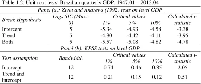
order to asses on unit root question, and verify whether the deterministic or stochastic trend is a better assumption for the Brazilian quarterly GDP time series. Table 1.2
shows the test results.
Table 1.2: Unit root tests, Brazilian quarterly GDP, 1947:01 – 2012:04 Panel (a): Zivot and Andrews (1992) tests on level GDP Break Hypothesis Lags SIC (Max.:
8)
Critical values Calculated t-statistic
1% 5% 10%
Intercept 5 -5.34 -4.93 -4.58 -3.38
Trend 5 -4.80 -4.42 -4.11 -3.95
Both 5 -5.57 -5.08 -4.82 -4.78
Panel (b): KPSS tests on level GDP
Test assumption Bandwidth Critical values Calculated t-statistic
1% 5% 10%
Intercept 12 0.74 0.46 0.35 2.05
Trend and
As we can see above, Panel (a) in Table 1.2 shows calculated t-statistics less than the
10% critical value for each one of the assumptions, that is, failing to reject the null of a unit root with a structural break. By its turn, Panel (b) displays KPSS tests rejecting the
null of stationarity in both assumptions. Consequently, all tests are confirming the existence of a unit root in the log-levels of the Brazilian GDP data, even when one takes account to the possibility of one structural change.
As the log-level of the Brazilian quarterly GDP is non-stationary around a stochastic trend, we can turn our attentions to the decomposition components, since the
HP-filter is able to remove up to four unit roots of a given series (see, e.g., Baxter and King, 1999; and Pedersen, 2001).
Figure 1.2, below, brings four series. First, part “a” shows the log-GDP time
series with CODACE recession dates illustrated in the shaded areas. Part “b” depicts our first average time series, namely, our results for the Brazilian GDP long-term trend
(solid line) and its two standard error bands (dashed lines). By visually inspecting Figure 1.2, one can clearly see a very smooth trend with a flatter slope after the 1980s. In fact, this reduction was remarkable: Brazilian long-term trend is now about 50%
times less steep than it used to be before the mentioned year.
According to Perron (1989), this type of smooth stochastic trend is
well-described as a unit root process with strong mean-reversion and fat-tailed distribution for the error sequences. As a result, most of shocks have a small, if any, long-term
Fig.1.2: Brazilian time series. (a) Log of Brazilian quarterly real GDP; (b) average trend series (solid line)
and two standard error bands (dashed lines); (c) average cycle series (solid line) and two standard errors bands (dashed lines); and, (d) average cycle series. Shaded areas are the CODACE recession dates.
Parts “b” and “c” also show that the trend and cycle components are less
accurately calculated during the periods of 1965-1970, and 1974-1980. These periods may be associated with many political and economic instabilities, such as the beginning of the Military Regime; a high and increasing inflation (in 1964 Brazilian General Price
Index - Internal Availability -reached a peak of 92% per year, for the whole 1947-1979 period); the extended slowdown in the GDP growth rate that Brazilian economy has
passed through during 1963-1967, due to a large package of restrictive fiscal and monetary policies, aiming to control the soaring prices; an even longer period of high
growth, over the 1968-1973 period, also referred as the Economic Miracle, in which the real GDP grew at a rate of 11% per year (Abreu, 1989); and, the break started around 1980. 1.6 2.0 2.4 2.8 3.2 3.6 4.0 4.4 4.8 5.2
50 55 60 65 70 75 80 85 90 95 00 05 10 (a) 1.6 2.0 2.4 2.8 3.2 3.6 4.0 4.4 4.8 5.2
50 55 60 65 70 75 80 85 90 95 00 05 10
-.20 -.15 -.10 -.05 .00 .05 .10 .15 .20
50 55 60 65 70 75 80 85 90 95 00 05 10
-.100 -.075 -.050 -.025 .000 .025 .050 .075 .100
50 55 60 65 70 75 80 85 90 95 00 05 10 (d)
(b)
Such sources of uncertainties would have affected the usual trend-cycle decomposition methods whenever it is assumed a particular specification for the
filtering procedure. However, as we argued before, the average component series should be more robust to them, since different decomposition outcomes can adapt faster to the
vast complexity of the real world economic time series.
In Figure 1.2, part “d”, we focus on the average cyclic series as well as on the CODACE recession dates (the Brazilian committee provides us the business cycle
chronology for the 1980-2009 period). Besides, one can notice a high degree of matching between both series. Still, in order to access an exact measure of their
correspondence, we need to transform our cyclic series in a binary indicator of the business cycle phases. For such, first, we find the turning point dates (peaks and troughs), and, second, we create our own dummy series, defining expansions as the
period from a previous trough to the most recent peak, and recessions as the period from a previous peak to the most recent trough.
In order to find the turning points, we employ a simple rule created by Wecker (1979), and also employed by Canova (1994) and Pagan (1997), among others, where a
peak is equal 1 when {Δyc,t> 0; Δyc,t+1< 0; Δyc,t+2 < 0}, where yc,t refers to the average
cyclic component. Conversely, a trough series is equal to 1 when {Δyc,t< 0; Δyc,t+1 > 0;
Δyc,t+2 > 0}. We also require that peaks and troughs alternate, so if two or more peaks
(troughs) are subsequent we select the one with a higher (smaller) value for yc. Thus, the
algorithm replicates a common view among media members and politicians that
Table 1.3 presents comparisons between our cyclic series and CODACE’s business cycle dates. This table also refers to the binary indicators for expansions and
recessions, S and tE S , respectively, derived from our decomposition after applying tR
Wecker’s (1979) rule. In a total of 120 quarters, our dummy indicator has a
correspondence rate of 86% ((79+24)/120) during expansions, and 88% ((44+61)/120) in recessions.
Table 1.3: Decomposition-CODACE comparisons, 1980:01 – 2009:04
Expansions Recessions
CODACE CODACE
E t
S 1 0 Total S tR 1 0 Total
1 79 8 87 1 44 11 55
0 9 24 33 0 4 61 65
Total 88 32 120 Total 48 72 120
Correspondence 86% Correspondence 88%
Moreover, while the errors in the course of expansions are quite similar, i.e., 8
cases in which our cycle series indicates a false upswing, and 9 cases in which it misses a real one; during recessions the average cyclic series misses only 4 in a total of 48
CODACE dates, i.e., a matching of 92%. Finally, it shall be noted that both series, S tR
and CODACE, are perfectly coordinated during the 1989:02-1992:01, 2002:01-2003:02 and 2008:03-2009:01 recessions.
In order to compare the performance of our method, we depict below, in Table 1.4, correspondence rates of other four different methods, using the same Wecker’s
unobservable components decomposition, considering that the cyclic component behaves as an AR(2), process (that is, UC(2) model).
As can be seen in Table 1.4, our averaged decomposition outperforms all the other methods, especially when it comes to expansions. Including, we have gotten
qualitative gains even when comparing with the classical HP-filter, the second best option. It is important to note that if one had means to check methods’ performance between 1965 and 1980, a period with large filtering instability, as Figure 1.2 shows, is
possible to think that our method could have obtained even better results.
Table 1.4: Comparative performance of decomposition methods
Filtering method Coincidence with CODACE in:
Expansions (%) Recessions (%)
Mean cycle 86 88
HP( =1600) 82 85
ARIMA(1,1,1)-BN 31 20
Baxter-King 75 76
UC(2) 73 73
1.4. Features of Brazilian cyclic component from 1947 to 2012
In order to examine features of the Brazilian business cycle, we divide the
sample into four distinct subsamples, namely, the years before the Military Regime, 1947-1963; the Military Regime itself, 1964-1984; the Democratic period before the Real Plan, 1985-1993; and the Real Plan period itself, 1994-2012.
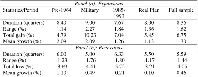
In Table 1.5, which brings patterns of the business cycle phases, the average duration, a measure of the phase length, is calculated using the formula
)
ˆ ˆ
1 /( 1
ˆi i i
In this case, parameters are obtained by the OLS regression Sti i iSti1, where i =
E, R, andS and tE S represent the same binary variables analyzed in Section 1.3. tR
By its turn, the average range during the business cycle phases, Âi, is estimated
as the slope of the linear regressions between ΔGDPt and S , and indicates the height of ti
expansions or the depth of recessions, in a given period of time. Having the mean duration and range, total gains and losses of the business cycle phases follow directly by
using the triangle approximation, CTi=0.5(Dˆi*Âi), where CTi refers to the cumulative
movements inside a cycle’s phase (aforementioned calculations follow Harding and
Pagan, 2002).
Expansions in Brazil last for approximately eight quarters, or two years, and recessions have a mean duration of six quarters, or 1.5 years. The three longest
expansions occurred from 1956:02 to 1961:02, related to the “Plano de Metas”, a
consistent and comprehensive plan of public investments; from 1967:01 to 1971:01 and
1971:04 to 1973:04, related to the Brazilian Economic Miracle period; and from 2003:02 to 2008:03, which was interrupted by the Great Recession.
On the other hand, the three longest recessions occurred from 1950:01 to 1953:02, related with unbalanced public accounts and a cambial crisis started around 1952; and the periods of 1981:01-1983:04, and 1989:02-1992:01, where political and
economic instabilities led to hyperinflation, and negative growth (Brazilian GDP reduced -4.25 in 1981, -2.93 in 1983, -0.06% in 1988, -4.35% in 1990, and -0.47% in
Table 1.5: Phase patterns, Brazilian business cycle Panel (a): Expansions Statistics/Period Pre-1964 Military
1985-1993
Real Plan Full sample
Duration (quarters) 8.40 9.00 7.67 8.00 8.36
Range (%) 1.14 2.27 1.84 1.36 1.62
Total gain (%) 4.79 10.23 7.04 5.45 6.75
Mean growth (%) 2.09 2.09 1.26 1.13 1.70
Panel (b): Recessions
Duration (quarters) 6.00 5.00 6.33 5.50 5.59
Range (%) -1.23 -1.76 -1.80 -1.17 -1.44
Total loss (%) -3.69 -4.41 -5.72 -3.21 -4.05
Mean growth (%) 1.10 0.49 -0.21 0.10 0.46
By closely inspecting Table 1.5, one can note that, while the business cycle
phases change across the subsamples, the duration of a full cycle is quite constant, around 3.5 years, i.e., 14 quarters. Another interesting fact is that the duration of expansions are longer than that of recessions, even during the 1980s. Additionally, total
gains are always higher than total losses, depicting a manifested asymmetry between the business cycle phases in the country. Besides, after the Real Plan, Brazilian economy
has had milder expansions and recessions (see total gain and loss, in Table 1.5), which shows some evidence of increased stability in the country since the mid-1990s.
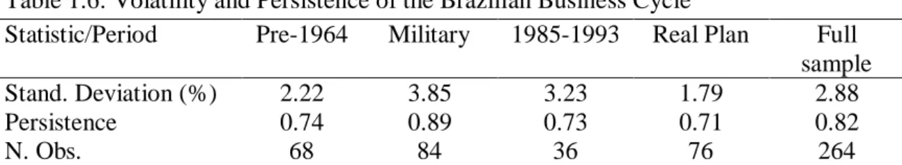
Persistence9, by its turn, has been quite stable in Brazil, usually oscillating around the 0.7-0.8 bands, as can be seen in Table 1.6. However, during some recessions, such as those occurred in 1989:02-1992:01, 1997:04-1999:01 and 2008:03-2009:01, the
cyclic series correlation has a tendency to reduce, probably due to a higher degree of uncertainty (as depicted by Figure 1.3, part “c”, below).
after 1994. In fact, the quarterly volatility after this year is less than half of that observed during the 1964-1984 period, and about 40% lower than its full sample value.
In order to make international comparisons, we can reproduce statistics calculated by Aguiar and Gopinath (2007) for a set of developed countries, who found standard
deviations in the order of 1.39% for Australia, 1.64% for Canada, 2.18% for Finland, 1.52% for Sweden, and 1.34% overall, between 1980 and 2003. Thus, after 1994, our results indicate that Brazilian instability may have been converging to a number
comparable to those estimated in some developed countries.
Table 1.6: Volatility and Persistence of the Brazilian Business Cycle
Statistic/Period Pre-1964 Military 1985-1993 Real Plan Full sample
Stand. Deviation (%) 2.22 3.85 3.23 1.79 2.88
Persistence 0.74 0.89 0.73 0.71 0.82
N. Obs. 68 84 36 76 264
Figure 1.3, below, provides additional information about Brazilian business cycles. In that figure, we estimate moving standard deviation, variance, and persistence of our cyclic series using a 14-quarter window, which is the same average duration of a
full cycle, besides the GDP 14-quarter mean growth-rate. These time series are depicted
in parts “a”, “b”, “c”, and “d”, respectively.
As one can see, parts “a” and “b” of Figure 1.3 confirm that Brazilian instability
has decreased since mid-1990s. Moreover, during periods of recessions, standard
deviation and variance tend to increase, but after the mentioned period, peaks of volatility are consistently lower than the previous one (the only exception is the last international crises peak). In this sense, all the evidence reported so far seems to support
authors for the U.S. economy (see, e.g., Kim and Nelson, 1999; McConnell and Perez-Quiros, 2000; and Stock and Watson, 2002).
Fig.1.3: Brazilian moving statistics: (a) standard deviation; (b) variance; (c) persistence; and, (d) GDP
growth rates. Note: moving window of 14 quarters, one full cycle period. Shaded areas represent CODACE recession dates.
According to Stock and Watson (2002), there are generally three main reasons for this phenomenon. The first one is related with structural changes that might have affected the economy; for example, the shift in output from goods to services (Moore
and Zarnowitz, 1986), improvements in the inventory management made possible by the advancements in information-technology (McConnell and Perez-Quiros, 2000), and
financial innovations that facilitates intertemporal smoothing of consumption and investment (Blanchard and Simon, 2001). The second reason would be improved monetary policy (e.g., Cogley and Sargent, 2005; Canova, 2009). And the third category
.00 .01 .02 .03 .04 .05
50 55 60 65 70 75 80 85 90 95 00 05 10
(a) .0000 .0005 .0010 .0015 .0020 .0025
50 55 60 65 70 75 80 85 90 95 00 05 10
(b) -1 0 1 2 3 4
50 55 60 65 70 75 80 85 90 95 00 05 10
(d) -0.2 0.0 0.2 0.4 0.6 0.8 1.0
50 55 60 65 70 75 80 85 90 95 00 05 10
is good luck, that is, a number of exogenous shocks that reduced U.S. volatility (Bernanke and Mihov 1998; Leeper and Zha 2003; Sims and Zha 2006).
Since the Real Plan implementation, Brazilian government has committed to foster a sustainable budget policy and the Central Bank’s monetary rules have
concentrated on price stability, especially after the adoption of the inflation targeting regime. Together, the more predictable monetary and fiscal policies and the
low-inflation scenario might be the reason why the current Brazilian macroeconomic
environment is less volatile. However, a consistent answer for this question is beyond the objectives of the present paper. Our focus is related to mapping process and raising
questions and characteristics which shall be explained by future investigations.
Additional information is found in Figure 1.3, part “d”. In the full sample, Brazilian economy has had 14 quarters of negative growth. The historical growth-rate
peak was found in 1973:04, which equals to 3.09% per quarter, while the lowest value occurred in 1983:03, equaling to –0.42% per quarter. Before the 1980s, the 14-quarter
growth rate of the GDP was swinging around 2% per quarter, a value closer to that believed as being the Brazilian natural growth-rate up to this year, which equals to 7%
per year, as pointed out in many sections of Abreu’s book (1989, p.222, for instance).
Since then, the Brazilian’s GDP long-term growth-rate seems to have converged to half
of this value, about 1% per quarter.
1.4.1. Robustness tests on the decreased volatility and structural change tests
other countries that had not yet been detected by previous papers. Specifically, we intend to examine if this finding is robust to changes in the volatility measure, and when
it has really happened.
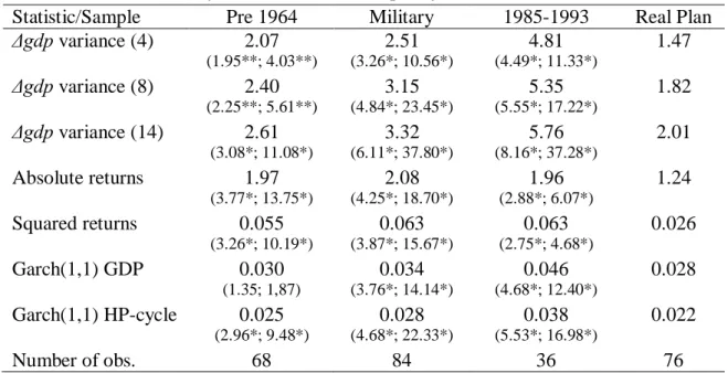
Table 1.7 brings a variety of proxies for the volatility in the country. The first
three series (“ gdp variance (i)”, i = 4, 8, 14) refer to the variance of the GDP log
growth-rate considering 4, 8 and 14 quarters moving windows, respectively. Next, two classical measures of instability are presented, i.e., the absolute and the squared returns.
Table 1.7 also shows the one step ahead forecasts of the conditional variance emerging from an ARIMA(7,1,0)-Garch(1,1) model for the log-GDP time series, and an
ARIMA(5,1,0)-Garch(1,1) model for the mean HP-cycle. Both specifications were chosen according to the Akaike (1987) information criteria, where, for the sake of simplicity, we assume normally distributed disturbances. Finally, we present, within
parenthesis, the classical Student’s t and Welch’s (1951) statistics for the null that the
estimated volatility in a certain period is equal to that found after 1994. Welch (1951)
test considers the possibility of different variances across subsamples10.
The first pattern seen in Table 1.7 is that volatility increased from 1947 to 1993 and then, after 1994, it fell to lower levels. On average, the instability of the 1994-2012
years is 28% lower than that observed during 1947-1963; 41% lower than that under the Military regime; and, 63% lower than the volatility of the 1985-1993 years. The major
difference across periods was measured by the variance of the growth rate within one year moving window, an approximation for the short-run volatility ( gdp variance, 4
order. Conversely, the minor differences were estimated by the Garch(1,1)-GDP proxy, wherein the instability after 1994 has decreased 7, 21, and 64%, relatively to the periods
in the same order as before. A second feature is that the period from 1985 to 1993, in which inflation levels were extremely high, was the most unstable in the Brazilian
history, for nearly all volatility measures11.
Table 1.7: More volatility statistics and mean equality tests
Statistic/Sample Pre 1964 Military 1985-1993 Real Plan
gdp variance (4) 2.07 2.51 4.81 1.47
(1.95**; 4.03**) (3.26*; 10.56*) (4.49*; 11.33*)
gdp variance (8) 2.40 3.15 5.35 1.82
(2.25**; 5.61**) (4.84*; 23.45*) (5.55*; 17.22*)
gdp variance (14) 2.61 3.32 5.76 2.01
(3.08*; 11.08*) (6.11*; 37.80*) (8.16*; 37.28*)
Absolute returns 1.97 2.08 1.96 1.24
(3.77*; 13.75*) (4.25*; 18.70*) (2.88*; 6.07*)
Squared returns 0.055 0.063 0.063 0.026
(3.26*; 10.19*) (3.87*; 15.67*) (2.75*; 4.68*)
Garch(1,1) GDP 0.030 0.034 0.046 0.028
(1.35; 1,87) (3.76*; 14.14*) (4.68*; 12.40*)
Garch(1,1) HP-cycle 0.025 0.028 0.038 0.022
(2.96*; 9.48*) (4.68*; 22.33*) (5.53*; 16.98*)
Number of obs. 68 84 36 76
Notes: *, **, *** denotes statistical significance at 1, 5 and 10% levels, respectively. Inside parentheses are t and Welch (1951) mean equality test statistics. All figures refer to the Brazilian quarterly data, 1947-2012, and are in percentages.
Throughout this paper, we have assumed a fairly logical division in the data set, beginning with pre-Military period, then the Military regime itself, passing through the
1980s and, finally, the Real Plan’s years. It seems to be a natural assumption, given the
recent political history of the country. Nonetheless, statistically, this type of a priori division of the sample makes the breakdate endogenous (correlated with the data), and
tests as those presented in Table 6 are likely to falsely indicate a break, when none in fact exists (Hansen, 2001).
11
In order to circumvent this difficulty, we apply three different classes of
methods, which are the Nyblom’s L test of structural changes with unknown breakdate
(Hansen, 1992), the Quandt (1960)-Andrews (1993) procedure, and the Hansen (2001) tests. The first one evaluates a structural change in all the parameters of a model,
without assuming a specific date, but it does not provide an estimated date of change. The Quandt (1960)-Andrews (1993) and Hansen (2001) methodologies, however, do estimate a breakpoint date, besides providing complementary pieces of information.
When computing Nyblom’s L test, we follow Hansen (1992) and McConnell and
Perez-Quiros (2000), assuming that the Brazilian GDP log-growth rates behave
according an AR(1) process with a drift. It is a simple yet powerful model, as showed by Hess and Iwata (1997). Proceeding in this way, we are able to test for breaks in the mean, in the autoregressive coefficient and in the variance of the time series, which are
associated, respectively, to structural changes in the trend, persistence and volatility of the GDP.
In order to calculate Nyblom’s L statistics for the null hypothesis of constancy in
the model’s parameters ( , ϕ, 2), first we need to run OLS estimation, and then define:
. 1 , ˆ ˆ , , , 1 , ˆ 2 2 m i e m i e x f t t it it (1.2)
Where, xit is equal to one, for the ’s case, and equal to gdpt-1 for the ϕ parameter’s
case; êt represents the OLS residuals; ˆ2 the OLS model’s variance; and m + 1 the total
of parameters estimated, in our case, m = 3. By OLS definition, equation (1.2) is
the OLS first order conditions (Hansen, 1992). Now, we define t1 ,
j ij
it f
S the
cumulative first order condition up to a given time t. Thus, by the first order condition, Sin = 0. Hansen (1992) provides two types of statistics, one for testing the stability of
each parameter individually, and other for testing the stability of all parameters jointly. For the single parameter case, test statistics are given by,
, 1 1 2 n t it i i S nV L (1.3) where, . 1 2 n t it i f V (1.4)
For the joint stability test, it is convenient to use matrix notation, that is,
n
t t t
c n L 1 1 ' , 1 S V S (1.5) where, . 1 ' n
t t t
V f f
(1.6)
first-order conditions. Under the null hypothesis, these cumulative sums will tend to wander around zero, but under the alternative, they will not, thus developing a nonzero
mean in parts of the sample, and leading to larger test statistics (Hansen, 1992).
Table 1.8 brings the output of Nyblom’s L test. In this table, we present five Panels; from “a” to “e”, in which Nyblom’s tests are applied to different samples. First, Panel (a) shows the method for the whole data set. In this case, the estimation shows a clear break in the trend, with a calculated statistics of 1.27 that can be compared to the
critical values of 0.47 (5%), or 0.35 (10%). Besides, we cannot find a significant break in the autoregressive parameter, and the variance presents a break only considering a
critical value of 10%.
However, we have seen before that the variance results during the pre-Military and the post-Real Plan periods are somehow similar, and this might be distorting the
tests. As presented in the table, if the sample is given in decades, the break in the variance becomes clearer, with the L statistic reaching a peak of 0.97 during the 1980s,
and 0.94 after the 1990s. Besides, as long as we move the sample as before, the structural change in the mean, , disappears after 1980, which indicates that the break may have occurred around this year.
Results from Table 1.8 for the autoregressive parameter are mixed, and they may not have suffered a major change during the period of the analysis of the sample, as
shown in Table 1.8 Panel (a), Table 1.6 and Figure 1.3.
Hansen (1992) tests are informative and have a solid statistical basis, but they
Quandt-Andrews), and the second one to Hansen (2001). Here we present the Quandt-Andrews test first, since Hansen (2001) utilizes some of its concepts.
Table 1.8: Nyblom’s L test for stability of Brazilian real GDP growth – 1947:01 to 2012:04
Specification: gdpt = + ϕ gdpt-1 + t
Panel (a): 1947:01 to 2012:04
Parameter Estimate Lc CV (5%; 10%)
0.0103 (0.00) 1.268 0.47; 0.35
ϕ 0.1525 (0.01) 0.274 0.47; 0.35
2
0.0003 0.363 0.47; 0.35
Joint Lc 1.7345 1.01; 0.85
Panel (b): 1960:01 to 2012:04
Parameter Estimate Lc CV (5%; 10%)
0.0087 (0.00) 0.7643 0.47; 0.35
ϕ 0.1837 (0.09) 0.3911 0.47; 0.35
2
0.0004 0.5634 0.47; 0.35
Joint Lc 1.5347 1.01; 0.85
Panel (c): 1970:01 to 2012:04
Parameter Estimate Lc CV (5%; 10%)
0.0078 (0.00) 0.6332 0.47; 0.35
ϕ 0.2073 (0.01) 0.5784 0.47; 0.35
2
0.0003 0.6917 0.47; 0.35
Joint Lc 1.7345 1.01; 0.85
Panel (d): 1980:01 to 2012:04
Parameter Estimate Lc CV (5%; 10%)
0.0056 (0.00) 0.1426 0.47; 0.35
ϕ 0.0764 (0.25) 0.1363 0.47; 0.35
2
0.0003 0.9688 0.47; 0.35
Joint Lc 1.1734 1.01; 0.85
Panel (e): 1990:01 to 2012:04
Parameter Estimate Lc CV (5%; 10%)
0.0073 (0.00) 0.1273 0.47; 0.35
ϕ -0.0651 (0.75) 0.3805 0.47; 0.35
2
0.0003 0.9422 0.47; 0.35
Joint Lc 1.2292 1.01; 0.85
Notes: P-values are within parenthesis. Lc is the statistic for a break point in each of the parameters listed
in the first column. CV is the critical value for both 5 and 10% of significance, according Hansen (1992).
Chow’s statistics for every point of the sample between two dates, say, t1 and t212.
Through this search procedure, the breakdate can be found either using the maximum of
the Chow’s statistics (the original Quandt’s test), or the exponential and average
statistics, for all Andrews (1993) and Andrews and Ploberger (1994) calculated tables of
critical values, while Hansen (1997) provided approximate asymptotic p-values. In this research work, we apply the maximum and the exponential statistics, standard in the literature, and presented below, in equations (1.7) and (1.8), respectively:
)). ( ( max 2 1 t F MaxF t t t
(1.7) . ) ( 2 1 exp 1 ln 2 1 t t t t F k ExpF (1.8)
When applying Quandt-Andrews tests, we assume two specifications, one for breaks in the AR(1) model, gdpt = + ϕ gdpt-1 + t, which tests for breaks in and ϕ,
and other for breaks in volatility, where the dependent variable is a variety of proxies for the Brazilian instability, most of them listed before, in Table 1.7; is a parameter
that refers to the average volatility, and υt is an error term. The positive point about this
approach it that it allows testing for breaks in a vast number of instability indicators.
Finally, Hasen’s (2001) test integrates both Hansen (1992) and Quandt-Andrews
methodologies in a single framework. Assuming, again, an AR(1) process for the Brazilian GDP log-growth rates, Hansen (2001) procedure estimates and tests the time
2
) by means of the maximum and exponential statistics. The results of Quandt-Andrews and Hansen (2001) tests are presented in Table 1.9.
Beginning with the break on the mean growth-rate of the process, , Table 1.9 shows that Quandt-Andrews method estimates it in the second quarter of 1980, while
Hansen (2001) estimates a break in the first quarter of the same year. Besides, MaxF and ExpF Wald statistics for both methods are highly significant. In this sense, based on the findings of the trend-cycle decomposition, and on these results, one can be quite
sure about the timing of the break on the trend: the first semester of 1980. The GDP’s log-growth rate was estimated at 1.8% per quarter, before 1980, and 0.7% after that
year, which is similar to the results found in Section 1.3. The evidence reported here agrees, therefore, with the Lost Decade view, which has imposed to the Brazilian economy a permanent slowdown in its rate of growth.
With respect to the autoregressive coefficient, Table 1.9 Panel (b) confirms our previous expectations, showing that at 10% of significance we cannot reject the null
hypothesis of constancy in the ϕ parameter. Specifically, MaxF statistic was calculated as 7.24, with a p-value of 14%, while ExpF was calculated as 1.37, with a p-value of 12%. By reviewing Tables 1.6 and 1.8 Panel (a), we are able to reach the same
conclusion.
Now, we shall turn attention to the volatility question. Additionally to the
proxies presented before, Panel (a) from Table 1.9 brings three moving variances of the cyclic series (HP-mean cycle series), for windows of four, eight and 14 quarters,
respectively, the “Moving var. cycle (i)”, with i = 4, 8, and 14. Almost all short-term