Portfolio Choice with a Correlated
Background Risk: Theory and Evidence
∗
Luc Arrondel
†and Hector Calvo Pardo
‡CNRS-DELTA§
September 2002
Abstract
We extend the static portfolio choice problem with a small back-ground risk to the case of small partially correlated backback-ground risks. We show that respecting the theories under which risk substitution ap-pears, except for the independence of background risk, it is perfectly rational for the individual to increase his optimal exposure to portfo-lio risk when risks are partially negatively correlated. Then, we test empirically the hypothesis of risk substitutability using INSEE data on French households. Wefind that households respond by increasing their stockholdings in response to the increase in future earnings un-certainty. This conclusion is in contradiction with results obtained in other countries.
So, in light of these results, our model provides an explanation to account for the lack of empirical consensus on cross-country tests of risk substitution theory that encompasses and criticises all of them.
∗This paper is strongly motivated by a common work with André Masson (Arrondel and Masson, 1996). The authors thank Rob Alessie, Jean-Marc Robin, Maximus Spadaro and two anymous referees for their comments on a previous version of the text. We acknowledge research support from CNRS and SEEUID. The second author acknowledges
financial support from the Bank of Spain.
†E-mail address: [email protected] ‡E-mail address: [email protected]
1
Introduction
There has been growing interest on the implications of incomplete markets for both theoretical and empirical questions. Especially, many puzzles in the economics andfinance literatures have motivated the development and appli-cation of the theory on portfolio choice with background risk with successful results.
More precisely, the development of portfolio choice theory with incom-plete markets has forced researchers to take into account the statistical prop-erties of the uninsurable component of individuals’ income risk in explaining the demand for risky assets. Because it is beyond the individual’s control, this income risk has been termed ’exogenous’ or ’background’ risk. Consider-ing different classes of risks, Pratt and Zeckhauser (1987) with ’properness’, Kimball (1993) with ’standardness’ and Gollier and Pratt (1996) with ’vul-nerability’, establish conditions on individuals preferences for substitutability between endogenous and exogenous risks. In these contexts, an investor will reduce his demand for risky assets if the risk on his income increases.
There are very recent empirical papers which study the impact of income uncertainty and precautionary motives on the structure of households’ port-folio. But these papers do not lead to the same conclusions. On Italian data, households facing uninsurable risk and future liquidity constraints will reduce their share of risky assets (Guiso et al., 1996) and increase coverage against the risks that can be avoided (Guiso and Jappelli, 1998). Vissing-Jorgensen (2002) alsofinds evidence that background risk reduces stock market partic-ipation in the United States. Hochguertel (1998) results for the Netherlands are inconclusive and those of Alessie et al. (2000) for the same country did not find a significant effect of income uncertainty on the demand for risky assets. But Arrondel and Masson (1996) obtained a different result with French data: if households are more exposed to risk (proxied by occupation sectors), they invest a greater proportion of their wealth in risky assets.1
These inconclusive empirical results forced us to carefully look at the hypotheses under which theoretical models predicted risk substitution. Pre-cisely, all the theoretical results were conditional on the independence be-tween the two risks (capital and income), implying no correlation. However,
1Arrondel and Masson (2002) obtain a similar conclusion with data of ”Patrimoine
recent but yet preliminary and incomplete research on this correlation shows that this hypothesis needs not be true.
In this paper we present an extension of the static portfolio model with undiversifiable income risk to take account of a non zero correlation. We identify conditions on the correlation under which the investor will ratio-nally respond by increasing his demand for risky assets to increased income uncertainty. As well, less stringent conditions under which risk substitution may obtain can be found conditional on the correlation. So, previous models are a particular case of our hypothesis. Then, we tested the hypothesis of risk substitution using recent data concerning risky investment behaviour in France. We found that French households respond by increasing their stock holdings in response to the increase in future earnings uncertainty. This conclusion being in contradiction with findings in other countries, could be explained by spatial differences in the correlation between risks as our first part theoretical extension suggests.
The paper is organized as follows: in section 2, we provide the theoreti-cal framework of portfolio choice under incomplete markets and present our extension of the model with a correlated background risk. We also lay down the main hypothesis to be tested. Section 3 presents salient data features and describes the measure of risk aversion and the households’ subjective perception of income risk measure. The empirical analysis uses the 1997 IN-SEE Survey on Wealth (”Patrimoine 97”) which combines data on financial assets with information on individual income risk assessments for a sample of 10,207 French households. In section 4, we examine portfolio choice to esti-mate the impact of changes in background risk on portfolio demands .Section 5 concludes.
2
Theory
Not enough attention has been paid to the statistical properties of back-ground risk both at the theoretical and empirical levels, particularly to the statistical relationship between background risk and excess financial return risk. However, from an empirical point of view, there are some exceptions.2
Heaton and Lucas (2000) perform a cross-sectional analysis of the subjec-tive correlation between these two risks. When non-diversifiable income risk
2For a list of different measures of the correlation between labor incomes and stock
is decomposed in different categories (wage, proprietary and housing) each of them has a different statistical correlation to financial returns risk: on average, wage income and returns to housing are negatively correlated with stock returns, whereas proprietary income is positively correlated.3
Davis and Willen (2000) perform an empirical study of the correlation in the vein of Heaton and Lucas (2000) but using a different decomposition criterion. They identify occupation-level components of individual income innovations, motivated by the results of Cocco et al. (2001) who found that the correlation between labor income innovations and equity return innova-tions rises with education. Their main conclusions coincide with those of the previous work: cross-sectional heterogeneity helps to explain observed heterogeneity in portfolio choice and the statistical properties of income in-novations with respect tofinancial return innovations are conditional on these heterogeneities.
Botazziet al. (1996) study the correlation offluctuations between human capital innovations and innovations on the return of assets for a cross-section of OECD countries. For instantaneous correlations, theyfind that wages and profits move in opposite directions for most OECD countries. However they do notfind a robust sign for correlations between human andfinancial capital innovations.
Motivated by these results, we extend the static model of portfolio choice to include a small partially correlated background risk. We are able to show that in the case of negative correlation between the labour income shocks and the excess financial return shocks, introducing an additive background risk to the standard portfolio choice problem would increase the proportion of stocks held by households even if we allow for risk substitution on the unhedgeable component of the background risk. Intuitively, the negative correlation can be interpreted as an uncontrollable implicit liability in risky assets that individuals tend to compensate by directly modifying their port-folio risk exposure in the sense of increasing it. Thus, we allow for risk substitution on the independent component of the background risk, but the hedging effect from the correlated component can dominate the substitution effect.
3But the subjective measure of the correlation depends on individuals’ characteristics
2.1
Portfolio Choice Models
In this section we review the standard static optimal portfolio composition approximation model for small risks and its extension to the presence of an independent small background risk. Then we review the theoretical condi-tions on the class of preferences or in the class of background risks considered, under which we observe substitution between risks. We extend the results of this literature to the case of a partially dependent small background risk. Finally we discuss how the sign and magnitude of the correlation conditions the theoretical predictions of the literature of risk substitution.
2.1.1 Complete Markets
Consider the problem4 of an agent that considers how to invest his current wealth w0 when there are only two assets available : a risky asset promising
to deliver tomorrow a random return er and a riskless asset promising the delivery of a sure returnr. The individual objective function is a continuous differentiable representation of his preferences that admit an expected utility form over final wealth wf. Denoting by α the amount of initial wealth that
is invested in the risky asset, byez ≡er−r the excess return of the risky asset over the riskless asset, and byw≡w0(1 +r)thefinal wealth had he invested
all his current wealth w0 in the riskless asset, we can write the solution α∗
to the individual optimization problem as :
α∗ ∈arg max
α Eu(w+αez) (1)
Define as V(α∗) = Eu(w+α∗ze) the value function of the agent evalu-ated at its optimal portfolio choice. Following Gollier (2001) and under the assumptions :
(i) The excess return riskez is small and alternates in sign, (ii)u(.)is differentiable,
(iii)Eez >0, (iv) lim
α→+∞V
0(α)<0(5), and
4Throughout the paper we will borrow the standard notation that is used in the theory
of choice under uncertainty. An excellent recent book by Gollier (2001) from which we borrow notation, surveys and clarifies old and recent developments on the theory of choice under uncertainty and its applications.
5Which is equivalent to requiring t→−∞lim u
0(t)
lim
t→+∞u
0(t) >
R
0zdF(z)
R
0zdF(z)
(v) The Taylor expansion is taken aroundk = 0using the parametrization
e
z =kEez+eε:Ez >e 0and Eeε= 0,
we can approximate the solution of the standard portfolio problem in the following way :
0<α∗ ' Eez
σ2
zAu(w)
<+∞
So that the individual invests a positively bounded amount of his total wealth in the risky asset which is larger the larger the excess return it promises, and smaller the higher the risk aversion or the higher the variance of it.6
2.1.2 Incomplete Markets
In this section we present the extension of the basic portfolio choice model to the presence of an uninsurable component of individual income called ’background risk’.7
If we consider that the individual second period income is non-diversifiable (labor market second period income, proprietary income, or illiquid housing investments), independent of excessfinancial return risk and we denote it by
e
y then the standard portfolio problem described above can be rewritten as :
b
α∈arg max
α Eu(w+αze+ey) (2)
As previously we can define the value function of the agent as W(αb) =
Eu(w+bαze+ey)when evaluated at his optimal choiceα.b Under the (adequately modified) assumptions that we used for the standard portfolio choice model, we can approximate for small background and endogenous risks, the solution to the previous problem as follows :
0<bα'−EezE{u 0[w+
e
y]}
E{eε2u00[w+ye]} <+∞
Which deserves some remarks :
lim
t→−∞u
0(t) = +∞or lim
t→+∞u
0(t) = 0or boundedness above or below of the domain of the
utility function.
6This optimal risky assets demand is similar to those of Arrow (1965) for a static
frame-work and Merton (1971) for a multiperiod model under specific assumptions (additively separable utility function across periods and lognormality of asset prices).
7The effect of uninsurable and unavoidable earnings risk on consumption and portfolio
(i) The denominator of this expression can be rewritten in the following way :
E{eε2u00[w+ e
y]}=E{eε2}Eu00[w+ e
y] +cov[eε2, u00] :
eε2 = (ze−Eze)2
So that E{eε2}=E{(ze−Eze)2
}=σ2
z.
Since we can show8that ifcov[eε2
, u00] = 0,wefind an analogous expression
to the approximate solution of the standard portfolio problem [1] where we will replace the index of absolute risk aversionAu(w)for the felicity function u(.), by an index of absolute risk aversion Av(w) for the felicity function
v(s) =Eu(s+ye), as defined by Kihlstrom et al. (1981)9 :
b
α' Eez
σ2
zAv(w)
So that the portfolio problem with background risk will be analogous to the standard portfolio problem except for the change in preferences. Questions on the magnitude or direction of the optimal portfolio composition change when a small background risk is introduced can be explained by differences in the absolute risk aversion parameter when the underlying utility function changes from u(.) to v(.).10
(ii) Observe that if we do not restrict the two risks to be statistically independent, it can happen that W0(
b
α)|bα=0 ≥ 0 and thus αb ≥ 0 even if
Ez <e 0.This is because now :
sign W0( b
α)|αb=0 =sign{Eez+
cov[z, ue 0]
Eu0 }
8Observe thatcov[f(eε), g(ey)] =E[f(eε)g(ye)]−E[f(eε)]E[g(ye)] where f(s) =s2, g(t) =
u00(w+t). From the independence between eε and ye we will have that E[f(eε)g(ey)] = E[f(eε)]E[g(ey)]if :
(i) f : (Eε,Ξε) → R+ borel measurable and bounded, since ∀ε ∈ Eε, f(ε) ≥ 0 and
M ax{f(ε), f(ε)}<+∞.
(ii) g : (Ey,Ξy) → R− borel measurable and bounded. Thus considering −g(t) =
−u00(w+t) > 0,∀t in a compact support bounds below the fuction −u00(w+t). It is
bounded above as well if we impose lim
t→+∞−u
0(t) = 0, which is a necessary condition to
obtain an interior solution to the portfolio problem.
(iii) We assume that botheεandyeare defined on the same probability space (Ω, A,P). These three conditions are sufficient to guarantee the independence between (Borel measurable) real functions of independent real random variables.
9It must be noted that the assumptions under which this approximation is true are the
same as for the standard portfolio problem, where we replace u(.) by the indirect utility functionv(.)of Kihlstromet al. (1981).
Since given that u00(.)<0,the cov[ez, u0]>0 is equivalent tocov[z,e ye]<0.
Meaning that if both risks are negatively correlated, it is rational for a risk averse individual to invest in the risky asset even if it generates a negative expected excess return, since the reason why he will invest in it is the partial insurance it provides against the exogenous risk. And conversely if cov[ez, u0] > 0 : it can be perfectly rational for the agent not to invest
in the risky asset even if it delivers a considerable positive expected excess return over the risk-free asset. The reason now is that investing in the risky asset increases considerably the global risk the individual suffers, through the positive covariance between the two risks. Not to invest is a way of reducing the global risk up to the level the individual wishes to be exposed optimally. It is obvious to say from the expression above that if cov[ez, u0] = 0, then for
the individual to be rational to invest in the risky asset even in the presence of background risk, the excess return must be positive just as in the standard portfolio problem. Thus,
(iii) Replacing function v(.) by function u(.) in the standard portfolio problem, we obtain parallel conditions at the boundary, necessary to the existence of an interior solution for the portfolio problem with a small back-ground risk.
Pratt and Zeckhauser (1987) were the first to capture the common wis-dom intuition that individuals should react by reducing their risky invest-ments whenever their income became riskier, and termed it ’risk substitutabil-ity’. Risk substitutability seeks conditions on the class of background risksye and/or on the class of preferences u(.), under which the optimal investment in risky assets whenfinal wealth is partly non-diversifiable,α,b is smaller than what the agent would optimally invest were this non-diversifiable component absent, α∗ :
α∗ ∈arg max
α Eu(w+αze)>bα∈arg maxα Eu(w+αez+ye)
According to our approximations of the optimal solutions in each of the two cases, we observe that it would be sufficient for α∗ > bα to have Av(w) > Au(w), for a small independent background risky.e For background risks not
necessarily small, given the global concavity of the problem, the condition for risk substitutability imposes a non-positive sign on the FOC of problem [2] when evaluated at the optimal solution of problem [1]:
Depending on the class of independent background risks under consideration, the different authors needed to impose different restrictions on individuals’ preferences for risk substitution behaviour to be observed.
Pratt and Zeckhauser (1987) established that introducing an independent background risk in the class of undesirable risks11, requires preferences to be ’proper’ in order to observe that the individual rationally reacts so as to substitute the increased exposure to the exogenous risk by reducing his exposure to the endogenous risk, i.e. decreasing his risky portfolio demand.
Kimball (1993) stated that if the felicity function of the individual sat-isfies the decreasing absolute risk aversion (DARA) and decreasing absolute prudence (DAP)12 restrictions, introducing an independent loss-aggravating background risk13 ye to the standard portfolio problem (1) should decrease the individual optimal holdings of the risky asset. Preferences satisfying the DARA and DAP restrictions are termed ’standard’ by Kimball14. This result is also true in a multi-period portfolio choice model.15
11A risk eyis undesirable at initial wealth wif and only ifEu(w+ey)≤u(w).This can
be restated in terms of the risk premiumρ:Eey ≤ρ.This set of risks are also known as expected-utility-decreasing risks. Intuitively, the agent is willing to pay more than their expected value to take a decision as if he were in a certain environment (according to a certain objective function).
12Kimball (1990) proposes to measure absolute prudence by the ratio p = −u000/u00.
Positive prudence implies precautionary saving and indicates the strength of precautionary motive: if people have decreasing prudence, precautionary saving declines as individual wealth rises. Intuitively, an individual behaves according to decreasing absolute prudence if, as he becomes richer, he is willing to pay a decreasing amount to make his optimal decision in the absence of uncertainty prevail under uncertainty.
13A riskyeis loss-aggravating when starting from initial wealthwif and only if it satisfies Eu0(w+ey)≥u0(w). Observe that this is equivalent toEye≤Ψ:Ψis the precautionary
premium as defined by Kimball (1990). The set of risks that satisfy this property for preferencesu(.)and initial wealthware called expected-marginal-utility-increasing risks. In intuitive terms, they are risks that make the agent willing to pay a smaller amount than its expected value in order to keep as optimal the decision prevailing before the risk introduced. Finally observe that if preferences are DARA, every undesirable risk is loss-aggravating.
14Kimball (1993) introduces also the concept of temperance (measured by the ratio t = −u0000/u000) which describes a desire to reduce total exposure to risk. Under the
condition of ”standardness”, temperance is greater than prudence which is also greater than absolute risk aversion under DARA (t > p > A).
15Some recent theoretical papers examine the joint consumption-portfolio choice
Finally Gollier and Pratt (1996)16 consider the most restrictive class of independent background risks (unfair risks17) and obtain the least restric-tive class of preferences under which the individual behaviour displays risk substitutability. Gollier and Pratt show that preferences must satisfy the condition of ’risk vulnerability’.18
Then observing that if preferences are DARA, every undesirable risk is loss-aggravating, Gollier and Pratt (1996) summarize the relationship be-tween the preference class restrictions as:
Standardness⇒Properness⇒Risk vulnerability⇒DARA
2.2
A Correlated Small Background Risk
In this section we extend the basic portfolio problem to allow for a small partially correlated background risk, borrowing from Elmendorf and
Kim-composition decision. Under ”standarness”, increase in background risk reduces demand for risky securities. Increase in saving is observed at the same time under more stricter conditions on preferences (under CRRA for example).
Koo (1995), extending Merton’s (1971) multi-period consumption-portfolio choice model to labor income uncertainty and liquidity constraints, shows numerically that if economic agents have constant relative risk aversion (CRRA), an increase in the variance of per-manent income shocks leads to a reduction in both optimal allocation to stocks and the consumption-labor income ratio.
More recently, Viceira (1999) considers a similar multi-period model for which he derives an approximate analytical solution. He finds ”that an mean-preserving increase in the variance of labor income growth reduces the investor’s willingness to hold the risky asset and increases her willingness to save” (if investor’s preference are described by CRRA instantaneous utility function and that labor income risk is independent of stock market risk). Moreover, he shows that consumer primarily reacts by extending precautionary saving and secondarily by reducing his risky portfolio (see also Campbell and Viceira, 2002, and Letendre and Smith, 2001).
16These two authors made two major contributions in this paper beyond its own original
scientific contribution. First, they synthesized and clarified the relation between previous papers on restrictions on preferences that captured the intuitively appealing notion of ’risk substitutability’. Second, they generalized them in the sense of extending their results to the more intuitive class of unfair risks, evidentiating the trade-offbetween restricting the class of preferences and restricting the class of background risks.
17A risk ey is unfair if and only if Eye≤ 0. This can be restated in terms of the risk
premium ρ:Eye≤0≤ρ. Observe that undesirable risks have noa priori restriction on the sign of their expectation, and thus include unfair risks as a particular class.
18Preferences are ’risk vulnerable’ if absolute risk aversion,A,is decreasing and convex.
ball (2000) its stylized specification. The crucial point is that the sign and magnitude of the correlation may exacerbate or counterbalance the opti-mal portfolio response to the introduction of a background risk, even under the assumptions on preferences or risks that guarantee risk substitutability (except independence). Intuitively, if we suppose that there is a negative correlation between the endogenous and the exogenous risk, introducing it in the agent’s program would generate an additional motive for holding the endogenous risk: insurance against the adverse realizations of the exogenous risk.
2.2.1 A Partially Correlated Small Background Risk.
We want to study the individual static portfolio decision problem when the two risks are statistically correlated. To do this we adopt the methodology of Elmendorf and Kimball (2000) to the simpler problem defined above although
e
y=y+e²+βze=eh+βez.So that allowing for β 6= 0 we allow for a non-zero correlation between a part of the undiversifiable labour income riskye−ehand the endogenous financial excess return risk ez. The program (2) of the agent is modified accordingly, to become:
bθ ∈arg max
θ Eu[w+θez+eh]
So that the optimal portfolio composition that satisfies the FOC which is necessary and sufficient will be:
bθ=αb+β
We are going to derive approximations of the solution for small correla-tions β and risks z,e eh by using a first order Taylor expansion on the FOC. We will use the indirect utility function of Kihlstrom et al. (1981) over the independent component ehof background risk ey to rewrite program (2) as :
bθ ∈arg max
θ Ev[w+θze] (3)
So that the FOC evaluated at the optimumα∗ of program (1) becomes of an indeterminate sign:
Proposition 1 : If we introduce a small partially correlated background risk into the standard portfolio problem, the optimal portfolio composition response depends, under the standard assumptions for risk substitutability, on the sign and magnitude of the small correlation between risks19.
Proof. Consider the FOC of the agent’s problem (3) and take afirst order Taylor expansion on the marginal indirect utility:
v0[w+αz+βz] =v0[w+αz] + (βz)v00[w+αz] +o(βz),∀z
Where o(βz) is a quantity that represents higher order terms ofβz that will tend to zero faster than βz asβz → 0. This approximation is then valid for bothβ andz small. We obtain the following expression after premultiplying byzboth sides of the approximation, taking expectations and evaluating the FOC approximation at the optimum of the standard portfolio problem (1):
Ez{zve 0[w+α∗ez+βze]} ≈ Ez{ezv0[w+α∗ze]}+βE
z{[ze]
2
v00[w+α∗ez]}
≈ Ez,h{ezu0[w+α∗ze+eh]}+βEz,h{[ez]2
u00[w+α∗ze+eh]}
Where the approximate equality follows from substituting the indirect utility v(.) by its direct utility representationu(.). Then the first term on the RHS corresponds to the effect of introducing an independent background risk on the optimal portfolio composition of the standard portfolio problem under the assumption of independence between the endogenous and the exogenous risk. But now, there is a second term the sign of which depends on the sign of the correlation β :
β < 0 =⇒Ez{ezv0[w+α∗ze+βez]}Q0 =⇒bθQα∗ (4) β ≥ 0 =⇒Ez{ezv0[w+α∗ze+βez]}≤0 =⇒bθ≤α∗
The importance of this proposition is to show that even if we impose conditions on preferences and on the independent component of background risks to observe risk substitution, we might not observe it if the correlation
19Te reader is referred to the appendix for a more intuitive and extensive interpretation
with the dependent component of the background risk is negative and suf-ficiently large. On the contrary, if both risks are positively correlated it is possible that we observe risk substitution under less stringent conditions on preferences or the class of background risks considered. Observe also that if the correlation is null, there is no correlated component of the background risk and the standard restrictions on preferences and background risks predict when risk substitution is to be obtained. Finally observe that the proposition does not deal with a proper ’increase in risk’20. Instead we have adopted the more comfortable assumption of introducing an additive background risk as it is standard in this type of literature.
2.2.2 A partially Negatively Correlated Background Risk.
Since we are interested in observing conditions under which individual agents rationally react to the introduction of partially non-diversifiable income risk by tilting up the fraction of initial wealth invested in stocks, we will just consider the case of negative correlation in this section. As the approximate solution (4) shows, in the case of positive correlation risk substitution is aggravated.
Proposition 2 : A decreasing absolute risk averse individual will tend to increase his optimal exposure to financial risks when a partially negatively correlated risk is introduced additively into his optimization program, provided the undiversifiable uncorrelated part of the exogenous risk is loss-aggravating.
Proof. The FOC of 2 is : Ez,h{zue 0[w+bθ e
z+eh]}= 0 ⇐⇒Ez{ezv0[w+bθ e
z]}= 0
by definition of the indirect utility function v(x) = Ehu[x+eh], and by the
independence between ez and eh. The FOC of 1 is : Ezu0[w + α∗ez] = 0.
Subtracting both expressions : Ez ³
e
z{v0[w+bθze]−u0[w+α∗ze]}´= 0. If for any possible realization of the random variable z we have that v0[w+bθz]−
u0[w + α∗z] = 0, the necessary and sufficient condition will be satisfied.
If eh is loss-aggravating we have that Ehu0[w+eh] ≥ u0[w] or equivalently
that v0[w]≥u0[w]. Thus for the sufficient condition to be true, we need that
20A step towards this direction has been undertaken by Eeckhoudtet al. (1996) which
w+bθz ≥w+α∗z,∀z or equivalently thatbθ≥α∗.Now sincebθ≡αb+β :β <0 we have that bα≡bθ−β >α∗
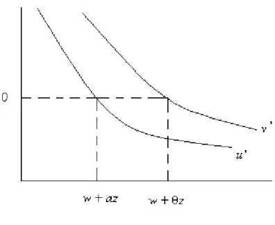
The intuition can be grasped infigure 1.
Figure 1: Intuition of the proof of Proposition 2
The following proposition extends the results of the first proposition on the effects of introducing a partially negatively correlated labor income risk (background risk) to the class of loss aggravating risks in which initial wealth is random.
Proposition 3 We can extend the previous proposition to the background risk ey being in the class defined as :
Eu0(w+α∗ez+ye)≥Eu0(w+α∗ze) (5) And the conclusion now will be thatα∗ <α∗−β ≤αb :β <0.Thus the optimal portfolio composition αb in the presence of the partially negatively correlated background risk ey will be higher than in the absence of any exogenous risk, and still bigger than the increase that would correspond to fully hedge the part of labor income risk that can be diversified using the financial markets.
Proof. The FOC of (2) is : Ez,h{ezu0[w+bθ e
z+eh]}= 0⇐⇒Ez{zve 0[w+bθ e
z]}= 0 by definition of the indirect utility function v(x) =Ehu[x+eh], and by the
independence between ez and eh. The FOC of (1) is : Ezu0[w+α∗ez] = 0.
Subtracting both expressions : Ez ³
e
z{v0[w+bθ e
z]−u0[w+α∗ e
z]}´= 0. If for any possible realization of the random variable z we have that
v0[w+bθz]
−u0[w+α∗z] = 0 (6)
the necessary and sufficient condition will be satisfied. If ey is in the class of loss-aggravating risks satisfying (5) we have thatEv0(w+θ∗ze)≥Eu0(w+α∗
e
z)
using the definition of the indirect utility function, withθ∗ ≡α∗+β :β <0. A sufficient condition guaranteeing that ye is in the class (5) is, taking the following definitionsωe ≡w+α∗ez,eε≡βez,
∀ω,ε:v0(ω+ε)≥u0(ω)
And particularly it must be true that :
∀ω :v0(ω+ minε)≥u0(ω)
Noting that we adopt the convention of signminε<0so thateε≡βezimplies that if β < 0 then minε ≡ min[βz] = β[maxz] < 0. Conversely, if β > 0
must alternate in sign for the portfolio problem to have a bounded solution. This observation will be used below.
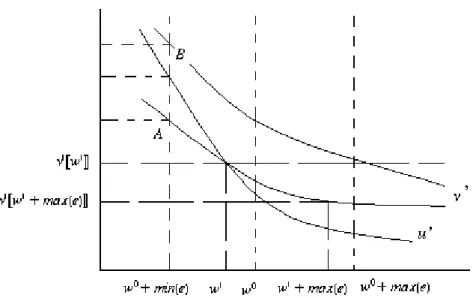
As depicted in figure 2, and using the fact that v00(.), u00(.) < 0 by risk
aversion, two situations are possible at any particular ω0:
Situation A is not possible since if u0(ω
0 + minε) > v0(ω0 + minε) ≥
u0(ω
0) then there must exist a ω1 < ω0 : v0(ω1) = u0(ω1) implying that
v0(ω
1+ maxε) < u0(ω1) by v00(.)< 0. A contradiction. Then only situation
B is possible imposing that:
v0(ω
0+ minε)≥u0(ω0 + minε),∀ω0,ε (7)
Now we will use condition [6] conveniently rewritten in terms ofω,εas follows for all possible values of z:
v0[w+ b
αz+βz+α∗z−α∗z]≡v0[ω+ε+ ( b
α−α∗)z] =u0[ω]
and plugging the last equality in the condition [7] :
v0(ω
0+ minε)≥v0
·
ω0+ [minε] + [minε] + (αb−α∗)
1
β [minε]
¸
By risk aversion, i.e. v00(.)<0, the previous inequality implies that :
[minε] + (αb−α∗)1
β [minε] =
1
β [minε] [β+ (bα−α
∗)] = [maxz] (bθ−α∗)≥0
or thatbθ−α∗ ≥0sincemaxz >0by convention. Thereforeαb≥α∗−β >α∗ for β <0.
3
The Data and the Risk Variables
We mostly rely here on the ”Patrimoine 97” household survey and on a specific part of the questionnaire devoted to the risk variable (either exposure or attitudes).
3.1
The ”Patrimoine 97” French Household Survey
A nationally representative sample of more than 10,000 households was drawn and a comprehensive interview survey of their wealth was conducted by the INSEE. It is an abridged version of the questionnaire from the earlier survey on ”Financial Assets 1992”. In particular it provides:
- detailed information on the socio-economic and demographic situation of the household (education, occupational group, marital status, information concerning the children...), as well as on the biographical and professional evolutions of each spouse (youth, career, unemployment or other interrup-tions of professional activity) ;
- detailed data on household’s income, on the amount and the composition of its wealth (including liabilities and professional assets) ;
- brief information on the inter-generational transfers received and be-queathed (financial helping out, gifts and inheritance) and more generally on the ”history of its wealth”.
More specifically, a part of the questionnaire tries to give us a general idea of individuals’ degree of exposure and aversion to risk, as subjectively per-ceived and assessed by them. It consists of a recto-verso questionnaire which was distributed to the interviewees at the end of thefirst interview. This page submitted to the whole sample of 10,207 households must be filled in indi-vidually by the interviewee and his/her spouse (if applicable) and returned by post to INSEE. Only 4,633 individuals answered to this questionnaire (corresponding to 2,954 households).
The content is slightly different for employed persons than for unemployed or non working persons. More specifically, it asks the former to assess their short and long-term risks of unemployment, as well as the likely change in their future income over the next 5 years. In addition, a simple two-stage lottery game enables us to divide the individuals into four groups according to their degree of relative risk aversion following the methodology of Barsky et al. (1997).
the amounts invested in 1997. The fraction of households with direct stock-holding is about 15 percent. More precisely, around 12 percent of households have listed shares, 1.4 percent have non-listed shares and 3.1 percent own employers’ shares. The proportion of households with indirect stockholding -mainly through mutual funds- is around 13.5 percent. It follows that the upper bound of (direct or indirect) stockownership in France is estimated to be around 23 percent of the population. The average amount invested in (direct) stocks is about 3,800 euros (25,000 euros among direct stockholders) and households invest on average 6,700 euros in stocks or in mutual funds (29,000 euros among owners).
A descriptive analysis (Arrondel and Masson, 2002) shows that stock-holding exhibits a humped-shaped pattern according to age, with a peak of 28 percent in the 50-59 age bracket and increases very sharply with the level of (financial) wealth, concerning 85 percent of the households in the top centile. Stockholders are better educated, more often self-employed or employees in the private sector. Moreover, the frequency of stockownership is higher for male-headed or two income recipient households, and also when parents themselves own(ed) stocks.
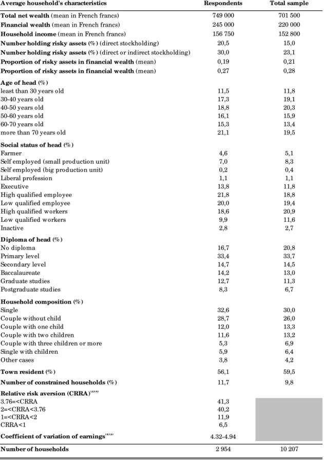
Table 2 reports descriptive statistics for the whole sample of 10,207 house-holds and for the sample of 2,954 respondents. There are only small dif-ferences between the two samples: the respondents seem to be older and more educated; they are more often white-collar workers and single and have less children; they are a little more wealthy (+ 6.7 percent for net wealth, +8.8% for financial wealth) and earn a little more money at work (+ 2.6 percent). A Logit model which estimates the differences between the two samples confirms these descriptive effects of wealth, social status, education and household composition.
These differences in socio-economic characteristics explain why the sam-ple of respondents own more often risky assets: the probability of owning risky assets is higher among the respondents than in the total sample (+5.5 percentage points for direct stockholding and +7 percentage points for di-rect or indidi-rect stockholding). But the average proportion offinancial wealth invested in risky assets is similar.21
21But, for the moment, we used the sample of respondents without taking into account
3.2
Measuring Relative Risk Aversion
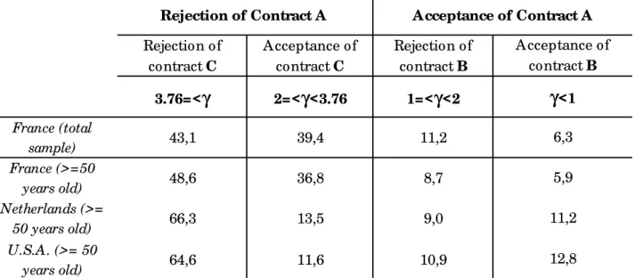
To obtain a measure of risk aversion, we asked individuals about their will-ingness to gamble on lifetime income (see the appendix) according to the methodology of Barsky et al. (1997). The ”game” resides in determining se-quentially whether the interviewee would accept to give up his present income and to accept other contracts, in the form of lotteries: he has one chance in two to double his income, and one chance in two for it to be reduced by one third (contract A), by one half (contract B), and by one fifth (contract C). This allows us to obtain a range measure of relative risk aversion under the assumption that preferences are strictly risk averse and utility is of the CRRA type. The degree of relative risk aversion is less than 1 if the individ-ual successively accepts contracts A and B ; between 1 and 2 if he accepts A but refuses B ; between 2 and 3.76 if he refuses A but accepts C ; and finally more than 3.76 if he refuses both A and C. Among the 4,633 respondents to the questionnaire, 3,483 individuals participated in the lottery.
Table 2 gives the fraction of all respondents who fall into the four risk aversion groups. Thefirst line gives the frequencies among the whole sample of respondents. The second line displays the frequencies amongfifty-year-old or more individuals. These results could be compared to those of Barsky et al. (1997) and those of Kapteyn and Teppa (2002) among the same age group (second and third line). As for the U.S. (76%) and the Netherlands (79.8%), most of the French respondents (85.4 percent) are in the category of high relative risk aversion (they refuse contract A). The main difference between France and the two other countries resides in the distribution between those who accept or refuse the contract C. In France, 57 percent of individuals who rejected contract A refuse contract C and 43 percent accepted this contract. However in the U.S. only 15 percent accept contract C and only 17 per cent do so in the Netherlands. Moreover, in France, only 6 percent accept contract B whereas in the U.S., as in the Netherlands, the acceptance rate is more than twice this rate (12.8 percent in US and 11.2 in Netherlands). In the U.S. and in the Netherlands there are more individuals with low relative risk aversion (inferior to 1).
risk aversion. You become more risk averse when you are older; a woman22; when your parents hadfinancial difficulties during your youth; when parents do not hold risky assets; and when people are educated. Finally and like in Barskyet al. (1997), wefind that risk tolerance decreases with income until the middle of the distribution, and then increases23.
We examine also the extent to which measured risk aversion predicts risky behavior (Arrondelet al.,2002): propensity to take risk infinancial decisions, participation in horse-betting type of games (horses race bets, national lotter-ies, slot machines, casino) and choice of occupational status (self-employed). Wefind that the risk aversion measure predicts all these risky behaviors, even after controlling for the economic and demographic variables: less risk averse individuals are those who are more willing to take risk in financial decisions, or to participate in national lotteries. Rather, doing racetrack bets or play-ing with a slot machine are related to intermediate risk averse individuals. Being self-employed (non farmer) is also influenced by CRRA: individuals who choose contract A are more often self-employed than the others.
3.3
The Self-Reported Measure of Future Income Risk
To construct a proxy for the subjective variance of households’ income (see the appendix), the methodology we followed is inspired in the survey car-ried out by the Bank of Italy, ” Survey of Household Income and Wealth ” (SHIW), for 1989 (Guiso et al., 1992). It asks households to distribute 100 points between different scenarios regarding the evolution of income - We as-sume that the household income variance can be proxied by the respondent’s estimated variance or, when there were two respondents in the household, by the head of the household variance evaluation24. So doing we obtain a measure of income uncertainty for 2,334 households. The average expected growth of future income is around 1.5%25.
22This gender-specific risk behaviour is also obtained by Barskyet al. (1997) but not
by Kaptein and Teppa (2002).
23The relationship between CRRA and wealth is ambiguous because the causality should
be the inverse (a more prudent consumer should save more). In Arrondel (2002), estimation of wealth equations shows no relation between asset holdings and CRRA.
24Assume thatfive years ahead expected real income isy
t+5=yt(1 + ¯x), the formula of the expected variance of household income isvar(yt+5)≡σ2y=σ2xyt2, whereytis current real income,x¯is the expected growth rate of real income andσ2
xits variance.
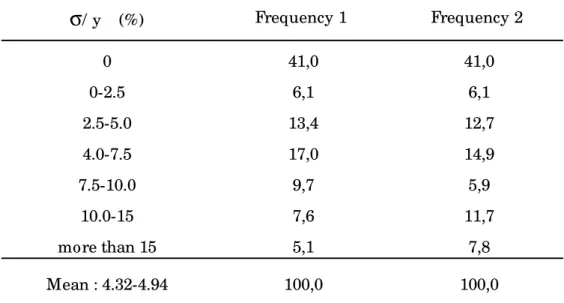
Table 3 displays the frequency distribution of the ratio between the sub-jective standard deviation and current income (σ/y). Two measures of risk are calculated depending of the value hold for upper and lower bounds (re-spectively 35 and 50%). More than forty percent of those surveyed hold point expectations about five year ahead expected real income. For almost half of them (46 percent) the standard error is between 0 and 10 percent (resp. 40%). Only 5 percent (resp. 8 percent) display a measure of uncertainty exceeding 15 percent. For the whole sample, the mean of the standard error of income shocks is about 4.3 percent (resp. 4.9) of the level of real income. The subjective income variance reported by French households is strikingly low when compared with the value usually assumed in the literature on pre-cautionary saving, reporting a value of the standard error of income shocks between 10 and 20 percent of the earnings’ level (for example 15 percent for next year expected earnings in the U.S. as reported in Deaton (1992). In the SHIW survey on 1989 Italian data, Guisoet al. (1992) obtain also a very low earnings variance for next year expected income; the standard error of earn-ings’ shocks being evaluated at 1.15 percent of current real earnearn-ings’ level. These authors put forward several reasons to explain the gap between the different measures: the nature of the data (self reported measure of earnings uncertainty and standard error of earnings uncertainty obtained from panel data); the possibility that Americans face more earnings uncertainty than Italians; overestimation of the true ”uncertainty” in econometric regressions or measurement error in cross section data.
A Tobit regression26 of (σ/y) on the sample characteristics shows that less risk averse households tend to report a higher variance. This result confirms that attitude towards risk affects job choice, with more risk averse households choosing safer occupations. We show that self-employed (except farmers) anticipate a higher income risk for the next five years. In other respects, it confirms that old households report a lower variance than young households corroborating that income profiles show decreasing risk along the life cycle. Households whose head is currently unemployed anticipate a higher risk on their future income like those who had or have health problems.
4
Empirical Analysis of Portfolio Choice
In this section, we use data from survey ”Patrimoine 1997” to study the impact of background risk and borrowing constraints on the demand for risky assets in France. The current analysis compares closely to that of Guisoet al. (1996) mainly in two respects: we assess income uncertainty from subjective information and we dispose of a similar measure of borrowing constraints.
4.1
Econometric Speci
fi
cations
We posit the following relation for the share of risky assets infinancial wealth: A
F =g(σ
2
, cl,γ, X) +e (8)
where A ≥ 0 is the demand for risky assets and F is total financial wealth. cl is the probability of being liquidity constrained in the future (see the appendix), σ2
is the subjective earnings variance, γ is coefficient of relative risk aversion and X is a vector of variables which influence the demand for risky investments. eis an error term. In specification (8) income risk is assumed to be exogenous as in recent models of portfolio choice.
The set of explanatory variables X has been chosen according to the theoretical models. In portfolio choice models where capital markets are imperfect (transaction costs, holding costs, imperfect information) portfolios are incomplete (King and Leape, 1998). So portfolio choice depends on household’s income and wealth (tofinance transaction and information costs) and on the stock offinancial information (proxied by age, education, parents’ wealth composition). We take into account other sources of future exogenous risk, especially on family (we control only by marital status and number of children at home or away from home). Finally, we introduce the nature of (present or past) professional activity (employee vs. self-employed).
less diversified portfolio than the old: the young are more likely to be liquidity constrained and so less willing to take risk when choosing their portfolio.
A simple OLS regression of (8) leads to inconsistent estimates due to the fact that a significant proportion of households does not own risky assets. In the same way, OLS regressions of (8) on the restricted sample of investors who hold risky assets is subject to selection bias (Heckman, 1976). So, I model the demand for risky assets as a two-stage decision process (King and Leape, 1998) where the first step is a Probit model to account for the probability of ownership and the second step consists in estimating conditional demand of risky assets (by introducing the opposite of Mill’s ratio in the set of regressors to correct selectivity bias). In other words, households choose first whether or not to hold risky assets, then they decide how to allocate total financial wealth between safe and risky securities. As there are only two categories of assets used in regressions, it is also possible to handle the selection bias by estimating a simple Tobit model on the share of risky assets where the lower limit is zero. However, Tobit estimation constrains to depend on the same set of variables, the determinants of whether to hold risky assets or not and if so how much.
In the two-stages procedure, we use different sets of explanatory variables to explain the discrete and the continuous choice. We assume that informa-tion costs explain essentially the decision to hold or not risky assets (Arrondel and Masson, 1990). Therefore we introduce education and the presence of risky assets in parents’ wealth only in the Probit model27. Moreover, this hypothesis guarantees that the opposite of Mill’s ratio is not co-linear with other explanatory variables of conditional demand.28
Tables 5 (a and b) and 6 (a and b) display results issued of the two econometric techniques. Column 1 and 2 of the tables show results of two-step estimation; column 3 displays results of Tobit estimation.
27Moreover, gains or loose in stock exchange investments have been introduced only in
the demand equation.
28For more details about estimation of household portfolio models, see Miniaci and
4.2
Demand for Risky Assets in France
4.2.1 Direct stockholding
Demand for risky assets, A, is firstly proxied by direct stockholding invest-ments. Columns 1 and 2 of Table 5a report two-step estimation results (discrete and continuous choice) using this definition of risky assets. The age variables indicate that the probability of risky assets ownership is the lowest for young households and increases through the life cycle to reach a maxi-mum at the age of 46: increases in probability of owning risky assets could be explained by information costs but the reduction in risky investments after 46 is more complex to interpret29.
The effect offinancial and total net wealth in the Probit model (and the effect of inheritance) is positive and is consistent with the presence of fixed transaction costs and a DARA utility function. An increase in the amount of financial net wealth from the 10th percentile (around 1,000 euros) to the 90th percentile (around 100,000 euros) increases the probability of being a stockholder by 17.1 percentage points, when holding the other variables in the regression constant at their means. The stock of information inherited from parents proxied by the ownership of the same assets in parents’ wealth increases also the probability of risky assets ownership (see also the positive effect of the head of household’s education, significant at 10%). Households whose parents owned stocks are about 10.6 percentage points more likely to hold stocks directly, again keeping the other regression variables constant at their means. Self-employed own less equities than other households. Single persons (except divorced), married couples or unmarried couples for less than 5 years invest more often in risky assets than other types of households.
The effect of individual measures of risk aversion has the expected sign in Probit but coefficients only distinguish great risk averters (CRRA= 3.76) from other risk averse households30. Households who are classified in the group of high risk averters were,ceteris paribus,about 6.7 percentage points less likely to hold stocks directly (relatively to the group of low risk averters). The coefficient of the proxy for liquidity constraints is negative in the Probit equation: households who anticipate to be liquidity constrained in the future
29Arrondel and Masson (1990) suggest that the decrease in the probability of owning
risky assets could be interpreted by deferred consumption needs (a life cycle motivation): to consume their wealth during retirement, old households prefer to hold liquid investments.
30However, the negative relation between risk aversion and demand for risky assets is
invest less in risky assets. Moving a household from the 10th to the 90th percentile of probability to be deterred from applying for credit in the future decreases the probability of being a stockholder by 7.6 percentage points, keeping the all other regressors fixed at their means.
Concerning human resources, we first note a positive mean-effect of non financial income on the probability of stock market participation. Moving a household from the 10th to the 90th percentile of labor income increases the probability of being a stockholder by 9.4 percentage points, keeping the all other regressors fixed at their means.
The coefficient of the expected variance of income31 in the Probit equation is negative and significantly different from zero: households whose future income is less risky are also those who invest less in risky assets. In other words, income risk and endogenous risk do not appear to be substitutes. Households who have no risk on their labor income were, ceteris paribus, about 3.6 percentage points less likely to hold stocks directly than households who are in the highest risky income decile.
There are few variables which are statistically significant in the condi-tional asset demand equation (column 2): large Stock Exchange gains in the past increase the amount invested in equities; entrust of financial advisors for managing portfolio increases the share of stocks in financial wealth. So, it appears that conditional demands for stocks are mainly explained by the variables which proxy price fluctuations on the capital market. We find a negative effect of income risk on conditional demands for risky assets but the coefficient is not significantly different from 0.32
To compare our results with Guisoet al. (1996) conclusions favoring the substitutability hypothesis (the coefficient of the expected variance of income is significantly negative), we run a Tobit model on the share of risky assets in financial wealth (column 3): the coefficient of income variance is always positive but it is only significant at 13% level.
Because retired people have no risk on their non financial income, we
31The value of subjective income variance introduced in the regressions corresponds to a
upper and a lower bound of 50% for the evolution of income. However, the results obtained are qualitatively the same with other future values.
32These results, combined with the previous ones concerning stock market participation
perform the same regression as the previous ones but only on the sample of households with an active head (Table 5b). The non financial income volatility effect is always negative on the probability of stock participation. It is negative in the Tobit model for the share invested in stocks. Active households who have no risk on their labor income were, ceteris paribus, about 5.2 percentage points less likely to hold stocks directly than active households who are in the highest risky income decile.
4.2.2 Robustness and miscellaneous results
Since only a small fraction of households report positive amounts of risky assets, we have also explored the sensitivity of the results to a broader defi ni-tion of risky assets: direct or indirect stockholding (Table 6a for total sample, Table 6b for an active head of household). For most variables, the estimates are similar to those obtained with the narrow definition. Notably, the coeffi -cient of income variance in the discrete choice hypothesis is always positive and statistically significant33; in the continuous choice, this coefficient is not significantly different from 0. In Tobit regressions, the coefficient is positive and significantly different from 0.
However, the previous estimates can be misleading (Lusardi, 1997). Some of the zero values in the self-reported measure of earnings variance may be artificial and may constitute a non negligible component of measurement error. Additionally, there could be an endogeneity bias, since more risk averse households might have chosen simultaneously safer jobs and less risky
33Households who have no risk on their labor income were, ceteris paribus, about 6
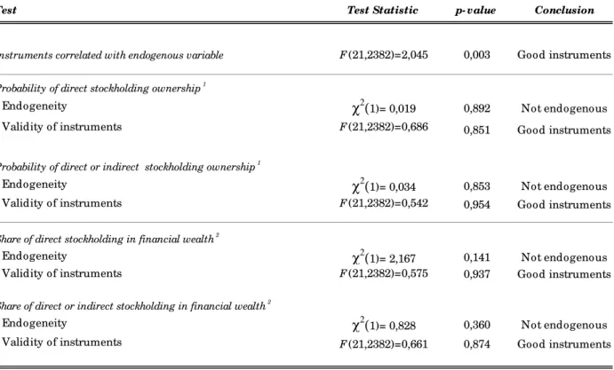
portfolios34. In these cases, the coefficient of earnings variance is biased35. We rigorously tested endogeneity by estimating an instrumental variables model in which the first stage regression predicts income risk using an OLS model, and the main equation predicts the probability of stock ownership using a linear probability model, or the share of stock in financial wealth using an OLS model. At the level of the household’s head, the instruments are the subjective probability of unemployment, the existence of previous health problems and a dummy for becoming independent; at the level of par-ents, they are proxies for resources, social status and portfolio composition. The results of specification tests concerning this econometric procedure are reported in Table 7.
We tested whether income risk is endogenous by including in the main equations both actual income risk and the error term from thefirst stage re-gression (see Robin, 2000). In the case of the probability of stockholding, the null hypothesis of exogeneity was not rejected. Therefore, the single equation models is preferred as long as the instruments are valid. The instruments are jointly statistically significant in thefirst regression (partial F-statistics were 2.045). Moreover, we did not reject the null hypothesis that the instruments can be excluded from the main equations. For the conditional risky assets demands, the conclusions are the same. In consequence, we can consider that the positive effect of income risk on risky assets portfolio is empirically
34Drèze and Modigliani (1966) claimed that individuals choose endogenously their job
also as a function of their risk preferences, given that they addressed a lifetime decision theoretic model. Since the choice of a job is endogenous and future wages are uncertain, we can interpret job choice as the investment in a risky asset, the return on which are future uncertain wages. Eeckhoudt and Gollier (2002) have recently studied this problem. Ifu(.)
shows DARA, DAP and P>2A then a household who chooses simultaneously his job and portfolio will be less exposed to portfolio risk than a household whose job is exogenous. The intuition of this result is clear: for the individual characterized by these preferences, both income and portfolio risks are substitutes in the sense that a risk averse individual who chooses simultaneously his portfolio risk and his occupation depending on his attitude towards risk will behave more conservatively than he otherwise would, had been his labour income completely diversifiable.
35For instance, Friedman (1957, p. 74-75) found some self-employed save less than other
robust.36
5
Conclusion
In this work we have tried to clarify the empirical lack of consensus on the cross-country different attempts to test risk substitution by means of an ex-tension of the static portfolio choice model with a partially correlated small background risk. We argued that a non-zero correlation, even if small, can counterbalance the theoretical prediction of risk substitution behaviour. For the case of a negative correlation, we have shown that it might be perfectly rational to increase individual exposure to financial risk in response to in-creased earnings uncertainty. Risk substitution is always present but the ’hedging effect’ dominates the risk substitution effect. Conversely, if the cor-relation is positive, risk substitution can be derived under less restrictive assumptions.
In any case, the purpose of the theoretical part was to show that the em-pirical analysis performed subsequently for the case of France is not at odds with results available for other countries (substitutability in Italy and US., no correlation in Netherlands), once aggregate correlations are considered and not necessarily controlled for. So, the strikingly different conclusions can be reconciled. Not being available an empirically satisfactory measure of aggregate correlation between the empirical measures for earnings and excess financial return risks, definite conclusions on the empirical relevance of risk substitution theory should be postponed until then.37
However, other possible explanations can account for the empirically de-tected effect, like the role of labor supply flexibility, the endogeneity of job choice, the strength of the welfare state benefits etc.
36If we consider that portfolio choice is made simultaneously to consumption choice,
wealth has to be consider also as an endogenous variable in the model. We have verified that taking account of the endogeneity of this variable do not invalidate the positive relation between risky assets demand and income risk.
37The paper of Vissing-Jorgensen (2002) is a good example of an empirical study which
Appendix
Intuition of Proposition 1.
To better grasp the intuition, we will proceed in two steps. In the first we will assume that the background risk is perfectly correlated with the endogenous risk, and we will interpret the optimal portfolio response to its introduction. The second step corresponds to the proof of Proposition 1. The interpretation of the results in that proposition is made in accordance with the results of step one.
Consider the truncated problem that obtains when the uncorrelated risk component eh is absent. This preliminary step can be interpreted as impos-ing an exogenous restriction on the amount of total wealth that must be invested/shorted in the financial market providing an excess return over the riskless asset ofβz.e Then the individual will adjust his initial risky position in the absence of this constraint, to counterbalance the effect of this restriction. The program would be:
θ∈arg max
θ Eu[w+θez]
The first order necessary and sufficient condition becomes :
Ez{zue 0[w+θez]}=Ez{zue 0[w+αze+βez]}= 0 (9)
If it is evaluated at the solution of [1] we can observe that by continuity of u(.), the sign of the expression is related with the sign of the correlation β :
signEz{ezu0[w+α∗ez+βez]}=−(signβ)
To see why, observe that for a small correlation β and/or a small riskz,e we can approximate the marginal utility component in [ 9] as :
u0[w+α∗z+βz]≈u0[w+α∗z] + (βz)u00[w+α∗z],∀z
Premultiplying by z on both sides and taking expectations, we can observe that the first term on the RHS coincides with the optimality condition of problem [1], so that it is null. The second term on the RHS coincides with the SOC of [1] times the correlation factor, and by concavity of u(.) will always be negative if the correlation is positive, and conversely :
So that we can conclude that :
β < 0 =⇒Ez{zue 0[w+α∗ze+βez]}>0 =⇒bα>α∗ β ≥ 0 =⇒Ez{zue 0[w+α∗ze+βez]}≤0 =⇒bα≤α∗
This shows that just considering the correlated part of background risk
e
y there will be a direct effect on the optimal portfolio composition α∗ that will depend on the sign of the correlation. Intuitively, this component cor-responds to a ’hedging effect’ if the correlation is negative, or to a ’portfolio composition constraint’ if the correlation is positive.
The Measure of Relative Risk Aversion
Suppose that you have a job which guarantees for life your household’s current income R. Other companies offer you various contracts which have one chance out of two (50%) to provide you with a higher income and one chance out of two (50%) to provide you with a lower income.
Are you prepared to acceptContract Awhich has 50% chances to double your income R and 50% chances that your income will be reduced by one third?
For those who answer YES : the Contract A is no longer available. You are offeredContract B instead which has 50% chances to double your income R and 50% chances that it will be reduced by one half. Are you prepared to accept?
For those who answer NO : you have refusedContract A. You are offered Contract C. which has 50% chances to double your income R and 50% chances that it will be reduced by 20%. Are you prepared to accept?
The Measure of Earnings Uncertainty
Within the next 5 years, your total household revenue (the rise in prices excluded) :
-... will have increased by more than 25% -... will have increased by 10 to 25% -... will have increased by less than 10% -... will be constant
-... will have decreased by less than 10% -... will have decreased by 10 to 25% -... will have decreased by more than 25%