Stochastic Models
for Assets Allocation under the Framework
of Prospect and Cumulative Prospect Theory
S. P. Sidorov,
Member, IAENG,
A. Homchenko, and V. Barabash
Abstract—This paper examines the problem of choosing the optimal portfolio for an investor with asymmetric attitude to gains and losses described in the prospect theory of A. Tversky and D. Kahneman. We consider the portfolio optimization problem for an investor who follows the assumptions of the prospect theory and the cumulative prospect theory under conditions on the stochastic behavior both of the portfolio price and the discount factor.
Index Terms—optimal portfolio selection; prospect theory; geometric brownian motion
I. INTRODUCTION
One of the classic problems of the portfolio investment theory is the following one: for a given set of assets with the known prices and distribution function of returns, to find an optimal portfolio. Portfolio is a set of assets with weights, the sum of which is equal to 1 (the budget constraint).
The classical theory of portfolio investment considers an investor with a concave utility function u. Let xT be the
(random) price of the portfolio at timet=T, and wbe the wealth of the investor at time t = 0. Then the problem of finding the optimal portfolio can be represented as follows:
E0(u(xT))→max (1)
under the constraint
E0(mxT) =w, (2)
whereE0(u(xT))is the expected value (at the timet= 0) of
utilityu(xT), the maximum is taken over all state of nature
at timeT,mis a discount factor.
In this paper we consider the problem of finding the optimal portfolio for an investor with asymmetric attitudes to gains and losses described in the prospect theory of A. Tver-sky and D. Kahneman [1]. Their paper contains a number of examples and demonstrations showing that under the conditions of laboratory experiments people systematically violate the predictions of expected utility theory. Moreover, they proposed a new theory — the prospect theory which can explain the behavior of people in decision-making under risk in those experiments in which the traditional theory of ex-pected utility failed. Cumulative prospect theory (CPT) was proposed in [2] and is the further development of prospect theory. The difference between this version and the original version of prospect theory is that cumulative probabilities are
Manuscript received February 19, 2015; revised March 4, 2015. This work was supported in the Russian Fund for Basic Research under Grant 14-01-00140.
S. P. Sidorov, A. Homchenko and V. Barabash are with Saratov State University, Saratov, Russian Federation. e-mail: [email protected]
transformed, rather than the probabilities themselves. Modern economic literature considers the cumulative prospect theory as one of the best models explaining the behavior of the players, the investors in the experiment and in decision-making under risk.
The paper [3] shows that the prospect theory can resolve a number of decision making paradoxes, but the author notes that it is not a ready-made model for economic applications. Nevertheless, recent years show increasing interest in the problems lying in the intersection of prospect theory and portfolio optimization theory. It should be noted, that due to the computational difficulties connected to the complexity of the numerical evaluation of the CPT-utility, there are not so many works devoted to the portfolio optimization problem under the framework of both prospect theory [4], [5] and cumulative prospect theory [6], [7], [8], [9], [10]. While the papers contain some numerical results, only simple cases (2-3 artificially created assets) of the portfolio selection problem are considered. Besides, most of the papers are based on the assumption that testing data are normally distributed. How-ever, it is well known that many asset allocation problems involve non-normally distributed returns since commodities typically have fat tails and are skewed.
The paper [5] tries to select the portfolio with the highest prospect theory utility amongst the other portfolios in the mean variance efficient frontier. Developing this idea, the work [6] shows that an analytical solution of the problem is mostly equivalent to maximising the CPT-utility function along the mean-variance efficient frontier.
First, we briefly present the main ideas of this theory, and then proceed to the problem of finding the function for the assessment of the prospects under some assumptions on the stochastic behavior of the discount factormand the portfolio price.
II. EU-, PT-ANDCPT-INVESTORS
A. Expected Utility Theory
The most popular approach to the problem of portfolio choice under risk and uncertainty is the expected utility hypothesis. For an introduction to utility theory, see [11].
Bernoulli [12] and later Von Neumann and Morgenstern [13] suggested a theory for choosing an outcome from a set of risky or uncertain outcomes by comparing the expected utility values defined on final asset position. It later came to be known as Expected Utility Theory (EUT). It has been used as a reference model to find the optimal solution in many areas of economics.
outcomes.xrefers to the element ofX. Let G={X, F, P} is probability space over X and let U : X → R denote a utility function such that the value of U(x)is a measure of the decision makers preference derived from the outcomex:
xy ⇔ U(x)≥U(y),
where x y means the outcome x is preferred at least as much as the outcome y. Thus, the relationship between wealth and the utility of consuming this wealth is described by a utility function, U(·). In general, each investor will have a different U(·). In expected utility theory, decision makers attitudes towards uncertainty are wholly modeled by the value of utility functions defined on final asset positions. Let fξ(x) be the probability density function of a random
variableξ.
Definition 1. The expected utility (EU) of the gameGis the expected value of the utility functions of possible outcomes weighted by the corresponding probabilities:
UEU(G) =
Z
X
U(x)fξ(x)dx.
The expected utility hypothesis states that the individual (EU-investor) will make decisions following the principle of maximizing the value of his expected utility.
An important property of an expected utility function is that it is unique up to affine transformations. That is, ifU(·)
describes the preferences of an investor, then so doesU∗(·) = c1U(·) +c2, where c1>0.
The range of reasonable utility functions should be re-stricted by economic reasoning. The expected utility function has the following properties:
1) positive marginal utility, i.e. U′(x)>0 for allx. 2) risk aversion; a necessary and sufficient condition for
risk aversion is that the expected utility function is concave, i.e.U′′(x)<0 for allx.
The most exploited type of utility functions is the power utility function defined by
U(x) = x 1−γ
1−γ,
whereγ ∈(0,1). Marginal utility is U′(x) =x−γ >0 for
allx >0. We have U′′(x) =−γx−γ−1<0 for allx >0.
B. Prospect Theory
Prospect theory (PT) has three essential distinctions from Expected Utility Theory:
• investor makes investment decisions based on deviation of his/her final wealth from a reference point and not according to his/her final wealth, i.e. PT-investor concerned with deviation of his/her final wealth from a reference level, whereas Expected Utility maximizing investor takes into account only the final value of his/her wealth.
• utility function is S-shaped with turning point in the origin, i.e. investor reacts asymmetrical towards gains and losses; moreover, he/she dislikes losses with a factor of λ >1as compared to his/hers liking of gains. • investor evaluates gains and losses not according to the
real probability distribution per ce but on the basis of the transformation of this real probability distribution, so
x v(x)
-4 -3 -2 -1 1 2 3 4
-7 -6 -5 -4 -3 -2 -1 1 2 3 4
λ= 2.25,α=β= 0.88
λ= 2.25,α=β= 0.5
λ= 2,α= 0.25,β= 0.75
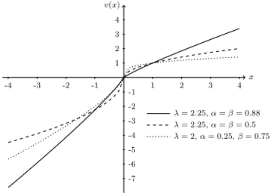
Figure 1. The plot of the value functionu(x)for differentα, β, λ
that investor’s estimates of probability are transformed in the way that small probability (close to 0) is over-valued and high probability (close to 1) is underover-valued. CPT includes three important parts:
• a value function over outcomes,v(·); • a weighting function over probabilities,ω(·);
• PT-utility as unconditional expectation of the value functionv under probability distortionω.
Definition 2. The value function derives utility from gains and losses and is defined as follows [2]:
v(x) = (
xα, if x≥0,
−λ(−x)β, if x <0. (3)
The fig 1. plots the value function for different values of α, β, λ. Note that the value function is convex over losses if 0 ≤ β ≤ 1 and it is strictly convex if 0 < β < 1. Moreover, the value function reflects loss aversion when λ > 1. It follows from the fact that individual investors are more sensitive to losses than to gains. D. Kahneman and A. Tversky estimated [1] the parameters of the value function α = β = 0.88, λ = 2.25 based on experiments with gamblers.
Definition 3. Letfξ(x)be the probability density function of
a random variableξ. The PT-probability weighting function
w: [0,1]→[0,1]is defined by
w(fξ(x)) =
(fξ(x))δ
((fξ(x))δ+ (1−fξ(x))δ)1/δ
, δ≤1 (4)
It is easy to verify that
1) w: [0,1]→[0,1]is differentiable on [0,1]; 2) w(0) = 0,w(1) = 1;
3) ifδ >0.28thenw is increasing on [0,1]; 4) ifδ= 1thenw(fξ(x)) =fξ(x).
In the following we will assume that0.28< δ≤1
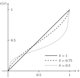
Fig. 2 presents the plots of the probability weighting function for different values ofδ.
Definition 4. The PT-utility of a gamble Gwith stochastic returnξis defined as [1]
UP T(G) =
Z ∞
−∞
v(x)w(fξ(x))dx, (5)
x w(x)
0.5 1
0.5 1
δ= 1
δ= 0.75
δ= 0.5
Figure 2. The plot of the probability weighting functionw(x)for different
δ
C. Cumulative Prospect Theory
We will consider the development of the prospect theory, Cumulative Prospect Theory, published in 1992 [2]. The description of CPT includes three important parts:
• a value function over outcomes, v(·);
• a weighting function over cumulative probabilities, w(·);
• CPT-utility as unconditional expectation of the value functionv under probability distortion w.
Definition 5. LetFξ(x)be cumulative distribution function
(cdf) of a random variable ξ. The probability weighting functionw: [0,1]→[0,1]is defined by
w(Fξ(x)) =
(Fξ(x))δ
((Fξ(x))δ+ (1−Fξ(x))δ)1/δ
, δ≤1 (6)
Definition 6. The CPT-utility of a gambleGwith stochastic returnξ is defined as [3]
UCP T(G) =
Z 0
−∞
v(x)dw(Fξ(x))−
Z ∞
0
v(x)dw(1−Fξ(x)), (7)
whereFξ(x)is cumulative distribution function ofξ.
If we apply integration by part, then CPT-utility of G defined in (7) can be rewritten as
UCP T(G) =
Z ∞
0
w(1−Fξ(x))dv(x)−
Z 0
−∞
w(Fξ(x))dv(x). (8)
III. SIMPLE STOCHASTIC MODEL
In this section we will suppose that the financial market consists of one risk-free and one risky assets. We examine the natural problem of how an investor optimizes her portfolio holding in a risky asset under PT and CPT with one risk-free asset and one risky asset with some assumption on the stochastic behavior of the discount factor and the risky asset price. The main goal is to compare solutions of this problem under PT and CPT assumptions with solution of the problem under Expected Utility Theory.
We will assume that the priceS of risky asset follows the standard lognormal diffusion process given by the stochastic differential equation known as Geometric Brownian Motion:
dS
S =µdt+σdz, (9)
whereµis a drift,σis a standard deviation,dz=ǫ√dt, the random variableǫis a standard normal,ǫ∼N(0,1).
We will assume that there is also a money market security that pays the real interest raterdt (risk-free asset):
dB
B =rdt. (10)
Following [14] we will assume that the discount factor Λ
follows the process dΛ
Λ =−rdt−
µ−r
σ dz, (11)
whereS is the price of the risky asset,ris risk-free rate. It is well-known [14] that the solution of (9) is
lnST = lnS0+
µ−σ
2
2
T+σ√T ǫ, (12) whereS0is the price of the risky asset at the moment 0,ST
is the asset price on the dateT. The solutions of (11) is
ln ΛT = ln Λ0− r+1 2
µ−r σ
2!
T−µ−r σ
√
T ε, (13)
whereε ∼N(0,1), and S0 is the price of the portfolio at
t= 0. It follows from (13) that mT =mT(ǫ) =
ΛT
Λ =
exp "
− r+1 2
µ−r σ
2!
T−µ−r σ
√ T ε
#
. (14)
LetW0denote the investor’s wealth at the timet= 0. Let
V denote the amount of money invested in the risky asset. ThenW0−V is the wealth invested in the risk-free asset. It
follows from (12) that the investor wealth WT on the date t=T is given by
WT = (W0−V)erT +V e(µ− σ2
2 )T+σ
√
T ǫ. (15)
Then the discounted value of the investor’s wealth is
f
WT =mTWT. (16)
Lemma 1. Leta∈R. Then
1
√
2π
Z
R
eaǫ−12ǫ2
dǫ=e12a2.
Proof:We have
1
√
2π
Z
R
eaǫ−12ǫ2
dǫ=√1
2π
Z
R
e−12(ǫ2
−2aǫ+a2)+1 2a
2
dǫ
=e12a2√1
2π
Z
R
The expected value at the momentt= 0of the discounted value of the investor’s wealth at the momentt=T is equal to
E0(fWT) = √1 2π
Z
R
e−
r+1 2(
µ−r σ )
2
T−µ−r σ
√
T ε
×
((W0−V)erT +V e(µ− σ2
2 )T+σ
√
T ǫ) e−12ǫ2
dǫ=
= (W0−V)e−
1 2(
µ−r σ ) 2 T 1 √ 2π Z R
e−µ−r σ
√
T ε−12ǫ2
dǫ+
+V e−
r+1 2(
µ−r σ )
2
T+(µ−σ22)T
× 1 √ 2π Z R
e−µ−r σ
√
T ε+σ√T ǫ−12ǫ2
dǫ=W0.
In the next subsections we examine the problem of finding the optimal portfolio (1)-(2) for three different types of investors: EU-investor with a power utility function, PT-investor, CPT-investor.
A. EU-investor with a power utility function
Suppose that EU-investor is maximizing the expected value of a power utility function. Then
UEU(V) := 1
√
2π
Z
R
WT1−γ
1−γe −12ǫ2
dǫ, (17)
whereWT is defined in (15).
Denote
f(V) := ((W0−V)e
rT +V e(µ−σ22)T+σ
√
T ǫ)1−γ
1−γ . (18)
The second order Taylor expansion of functionf(V) about 0 is
˜
f(V) =f(0) +f′(0) 1! V +
f′′(0)
2! V
2. (19)
Let us denote
˜
UEU(V) := √1 2π
Z
R ˜
f(V)e−12ǫ2
dǫ, (20)
We will examine the problem for the maximization of
e
UEU(V)overV, ˜
UEU(V)→ max
V∈[0,∞). (21)
Theorem 2. Letµ≥r. Then there is a unique solutionV∗
of the problem (21)defined by
V∗= W0 γ
−1 +e(µ−r)T
1−2e(µ−r)T +e2(µ−r)T+σ2T, V∗≈ W0
γ µ−r
σ2 .
(22)
Proof: We have f′(V) = ((W
0−V)erT +V e(µ− σ2
2)T+σ
√
T ǫ)−γ× (−erT+e(µ−σ22)T+σ√T ǫ) (23)
and
f′′(V) =−γ((W
0−V)erT +V e(µ− σ2
2 )T+σ
√
T ǫ)−γ−1× (−erT+e(µ−σ22)T+σ√T ǫ)2. (24)
Substituting (23) and (24) into (19) and (17) we get
e
UEU(V) = √1 2π
Z
R
(W0erT)1−γ 1−γ e
−12ǫ2dǫ+
V(W0erT)−γ
√
2π
Z
R
(−erT +e(µ−σ22)T+σ
√
T ǫ)e−12ǫ2dǫ−
V2(W
0erT)−γ−1
γ√2π
Z
R
(−erT +e(µ−σ22)T+σ√T ǫ)2e−12ǫ2
dǫ
(25) ThenUe′
EU(V) = 0 is equivalent to V = 1
γW0e rTA
B, (26)
where A = √1
2π
R R(−e
rT +e(µ−σ22)T+σ√T ǫ)e−12ǫ2
dǫ and B = √1
2π
R R(−e
rT + e(µ−σ22)T+σ
√
T ǫ)2e−12ǫ2dǫ. Using
Lemma 1 we have A=−√1
2πe rT
Z
R
e−12ǫ2
dǫ+
e(µ−σ22)T 1
√ 2π Z R eσ √ T ǫ e−12ǫ2
dǫ=
=−erT +e(µ−σ22)T+σ2
2T =−erT +eµT. (27)
and
B=e2rT√1
2π
Z
R
e−12ǫ2
dǫ− −2erT+(µ−σ22)T√1
2π
Z
R
eσ√T ǫe−12ǫ2
dǫ+
e2(µ−σ22)T√1
2π
Z
R
e2σ√T ǫe−12ǫ2dǫ=
=e2rT −2erT+(µ−σ22)T+σ2
2T +e2(µ−
σ2
2)T+2σ2T =
e2rT −2erT+µT +e2µT+σ2T. (28) It follows from (26), (27), (28) that
V∗= 1 γW0
erT(−erT +eµT)
e2rT −2erT+µT +e2µT+σ2T = 1
γW0
−1 +e(µ−r)T
1−2e(µ−r)T+e2(µ−r)T+σ2T.
Sinceex≈1 +xfor a smallxwe get V∗≈ 1
γW0 µ−r
σ2 .
Note that Ue′′
EU(V)≤0 for allV and therefore V∗ defined
by (22) is the solution of the problem (21).
B. PT-investor
For both PT-investor and CPT-investor we will assume that reference level of wealth at the time momentt=T isX =
W0erT, i.e. X is the amount of wealth the investor would
have received on the datet=T after investingW0 with the
continuously compounding rater. Then the deviation from reference pointX on the datet=T is equal to
DT(V) =WT−X =V ·(e(µ− σ2
2 )T+σ
√
T ǫ
−erT). (29) The allocation problem for PT-investor can be stated as follows:
UP T(DT(V))→ max
Let ǫ∗ be such that e(µ−σ2/2)T+σ√T ǫ∗
= erT i.e. ǫ∗ = −(µ−r−σ2/2)T
σ√T , or ǫ∗=
−µ−σ r+σ 2
√
T . (31)
Note that if V 6= 0 then D(V) ≥0 if the random ǫ ≥ǫ∗, andD(V)<0 otherwise.
Denote A1=
Z +∞
0
(eσ√T x−1)αw(f(x+ǫ∗))dx,
A2=
Z +∞
0
(1−e−σ√T x)βw(f(
−x+ǫ∗))dx, where
f(ǫ) = √1
2πe −12ǫ2
dt (32)
is the normal density function.
Theorem 3. Ifα < βthen there exists a unique solutionV∗
of the allocation problem (30),
V∗=e−rT
1
λ α β
A1
A2
1
β−α
. (33)
Proof: It follows from definition 4 that PT-utility of decisionV can be written as follows:
UP T(V) =
Vα
Z +∞
ǫ∗
(e(µ−σ22)T+σ√T ǫ
−erT)αw(f(ǫ))dǫ−
−Vβλ
Z ǫ∗
−∞
(erT −e(µ−σ22)T+σ
√
T ǫ)βw(f(ǫ))dǫ.
(34) Changing variables byǫ=x+ǫ∗ andǫ=−x+ǫ∗ in the first and the second integrals respectively, we get
UP T(V) =
VαeαrT
Z +∞
0
(eσ√T x−1)αw(f(x+ǫ∗))dx− −λ·VβeβrT
Z +∞
0
(1−e−σ√T x)βw(f(
−x+ǫ∗))dx. The allocation problem (30) can be rewritten as
VαeαrTA1−λ·VβeβrTA2→ max V∈[0,+∞).
We have U′
P T(V) =αVα−1eαrTA1−λβVβ−1eβrTA2= 0
at pointV∗=e−rT1 λ α β
A1
A2
1
β−α
. Moreover, U′′
P T(V∗) =
−α(α−1)Vα−2eαrTA
1+β(β−1)Vβ−2eβrTA2<0
if and only if α < β.
While the reference point X = W0erT depends on the
initial wealth W0, the deviation from the reference point
D(V) does not depend on W0. Therefore, as it is shown
in (33) the optimal amount to invest in the risky asset V∗ does not depend on W0.
Corollary 1. Letα < β. Then dVdλ∗ <0 and ifλ→ ∞then
V∗→0.
The corollary shows that the weight of risky asset in the portfolio is decreasing with increasing loss aversion.
C. CPT-investor
The allocation problem for CPT-investor can be stated as follows:
UCP T(DT(V))→ max
V∈[0,∞), (35)
whereDT(V)is defined in (29).
Letǫ∗ be defined in (31). Denote F1=−
Z +∞
0
(eσ√T x−1)αdw(1−Φ(x+ǫ∗)),
F2=
Z +∞
0
(1−e−σ√T x)β
dw(Φ(−x+ǫ∗)), where
Φ(ǫ) = √1
2π
Z ǫ
−∞ e−12t2
dt (36)
is the normal cumulative distribution function.
Theorem 4. Ifα < βthen there exists a unique solutionV∗
of the allocation problem(35),
V∗=e−rT
1
λ α β
F1
F2
1
β−α
.
Proof: It follows from definition 6 that CPT-utility of decisionV can be written as follows:
UCP T(V) =
−Vα
Z +∞
ǫ∗
(e(µ−σ22)T+σ
√
T ǫ
−erT)αdw(1−Φ(ǫ))−
−Vβλ
Z ǫ∗
−∞
(erT −e(µ−σ22)T+σ√T ǫ)β
dw(Φ(ǫ)), (37) whereΦ(ǫ)is the normal cumulative distribution function.
Changing variables byǫ=x+ǫ∗andǫ=−x+ǫ∗ in the first and the second integrals respectively, we get
UCP T(V) =
−VαeαrT
Z +∞
0 (eσ
√
T x
−1)αdw(1−Φ(x+ǫ∗))− −λ·VβeβrT
Z +∞
0
(1−e−σ√T x)β
dw(Φ(−x+ǫ∗)). The allocation problem (35) can be rewritten as
VαeαrTF1−λ·VβeβrTF2→ max V∈[0,+∞).
We have U′
CP T(V) =αVα−1eαrTF1−λβVβ−1eβrTF2= 0
at pointV∗=e−rT1 λ α β
F1
F2
1
β−α
. Moreover, U′′
CP T(V∗) =
−α(α−1)Vα−2
eαrTF1−β(β−1)Vβ−2eβrTF2<0
if and only ifα < β.
Corollary 2. Letα < β. Then dVdλ∗ <0and ifλ→ ∞then
V∗→0;
The corollary shows that the weight of risky asset in the portfolio is decreasing with increasing loss aversion.
0.025 0.05 0.075 0.1
1 2 3
µ, drift
δ= 1, PT and CPT investors
δ= 0.75, PT investor
δ= 0.75, CPT investor
δ= 0.5, PT investor
δ= 0.5, CPT investor
Figure 3. The dependence ofµonV for PT- and CPT- investors and differentδ
IV. COMPARATIVEANALYSIS OFEU-, PT-AND
CPT-INVESTORS
The problem solution for the EU-investor is similar to the solution of classical Merton portfolio choice problem where returns are assumed to be normally distributed, and the investor has the Constant Relative Risk Aversion utility (CRRA utility) [15]. This optimal portfolio has two main components: µ−r
σ2 is a measure of the investments in the
risky asset (defined as the Sharpe ratio divided by the standard deviation σ), and λis a measure of the curvature of the CRRA investor’s utility function. Therefore, the PT-and CPT-optimal portfolios have 2 components that play approximately the same roles as the ones represented in the EU-solution: the value of λ1αβA1
A2
1
β−α
(or λ1αβF1
F2
1
β−α
for CPT-investor) can be seen as a risk-reward measure and the parameters α and β are related to the curvature of the value function on the positive and negative domains, respectively [9]. However, these two frameworks (as PT-and CPT- investors have the same basis) have significant differences based on the specific features of the mentioned components. Furthermore, taking into consideration all the components included in the final solutions it can be stated that the main difference between PT- (CPT-)investor and EU-investor is that the former is dependent on the EU-investor’s wealth W0 at the time t = 0 but is not influenced by the
time factorT. Vice versa is correct for the latter.
Figure 3 presents the dependance of µ on V for PT-and CPT- investors PT-and different δ. We can see that V is increasing with increase of µ. The choices of optimalV for PT- and CPT-investors coincide in case δ = 1. The CPT-investor is more cautious than the PT-CPT-investor, as his choice of the optimal value of V is always less than the optimal choice ofV for the PT-investor in case δ <1.
Figure 4 presents the dependance ofσonV both for PT-and CPT- investors for different values ofδ. We can see that V is decreasing with increase ofσ. The choices of optimal V for PT- and CPT-investors coincide in caseδ= 1. Again, we can conclude that the CPT-investor is more cautious than the PT-investor, as his choice of the optimal value of V is always less than the optimal choice ofV for the PT-investor in caseδ <1.
0.05 0.1 0.15 0.2
0 1 2 3
σ, volatility
δ= 1, PT and CPT investors
δ= 0.75, PT investor
δ= 0.75, CPT investor
δ= 0.5, PT investor
δ= 0.5, CPT investor
Figure 4. The dependtnce ofσ on V for PT- and CPT- investors and differentδ
V. CONCLUSION
The paper deals with the problem of optimal portfolio choice for PT- and CPT- investors described in [10]. We have considered a simple stochastic model with one risk-free asset and one risky asset that follows geometrical Brownian motion stochastic equation. It turned out that if the parameters α, β of the value function u(·) satisfy the inequality α < β then there exists a non-trivial optimal choice for the weights of the assets. It is consistent with the findings of [9].
REFERENCES
[1] D. Kahneman and A. Tversky, “Prospect theory: An analysis of decision under risk,”Econometrica, vol. 62, pp. 1291–1326, 1979. [2] A. Tversky and D. Kahneman, “Advances in prospect theory:
Cumu-lative representation of uncertainty,”Journal of Risk and Uncertainty, vol. 5, pp. 297–323, 1992.
[3] N. C. Barberis, “Thirty years of prospect theory in economics: A review and assessment,”Journal of Economic Perspectives, vol. 27, no. 1, pp. 173–196, 2013.
[4] F. J. Gomes, “Portfolio choice and trading volume with loss-averse investors,”Journal of Business, vol. 78, pp. 675–706, 2005. [5] H. Levy and M. Levy, “Prospect theory and mean-variance analysis,”
The Review of Financial Studies, vol. 17, pp. 1015–1041, 2004. [6] T. A. Pirvu and K. Schulze, “Multi-stock portfolio optimization under
prospect theory,”Mathematics and Financial Economics, vol. 6, no. 4, pp. 337–362, 2012.
[7] V. Zakamouline and S. Koekebakker, “A generalisation of the mean-variance analysis,” European Financial Managements, vol. 15, pp. 934–970, 2009.
[8] X. D. He and X. Y. Zhou, “Portfolio choice under cumulative prospect theory: An analytical treatment,”Management Science, vol. 57, pp. 315–331, 2011.
[9] C. Bernard and M. Ghossoub, “Static portfolio choice under cumula-tive prospect theory,”Mathematics and Financial Economics, vol. 2, pp. 277–306, 2010.
[10] N. C. Barberis and M. Huang, “Stocks as lotteries: The implications of probability weighting for security prices,”American Economic Review, vol. 98, pp. 2066–2100, 2008.
[11] L. Eeckhoudt, C. Gollier, and H. Schlesinger,Economic and financial decisions under risk. Princeton: Princeton University Press, 2005. [12] D. Bernoulli, “Exposition of a new theory on the measurement of risk,”
Econometrica, vol. 22, p. 2336, 1954.
[13] J. von Neumann and O. Morgenstern,Theory of Games and Economic Behavio. Princeton and Oxford: Princeton University Press, 1944. [14] J. H. Cochrane, Asset Pricing. Princeton and Oxford: Princeton
University Press, 2005.