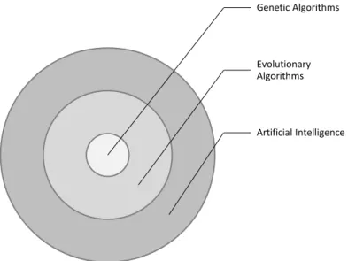
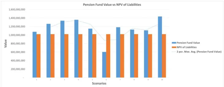
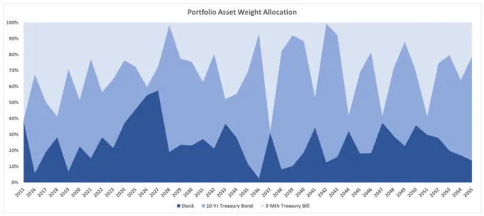
GENETIC ALGORITHMS APPLIED TO ASSET LIABILITY MANAGEMENT

Os autores concluiram que a flexão de cúspide gerada pela contração de polimerização, e a integridade de união não apresentaram diferança entre os

The acoustic beam generated by a circular plane piston was measured and compared to the results obtained by the exact and discrete solutions.. Both exact

To determine whether a variable in the sketch query may be referring to a group of contiguous regions, we analyse the solutions generated during the initial

The two points considered at the alternate sides, of the tangents through the diameter of the circle, and then the line joining these points divides the circle

By examining the impact on growth (enhancement or suppression) we generated ‘‘cross-species’’ genetic interaction profiles. We compared these profiles to the published

Todorov, pero más interesa trabajar sobre las diferencias entre conceptos fundamentales de la poética griega como el de mímesis y el de narrativa (en este sentido, J .L. B RAnDãO

Regarding the use of advanced modulation formats, it is proposed testing the NRZ channels used in the proposed architecture (at 1.25 Gbps and 2.5 Gbps) along with the

A idade revelou ser um fator preditivo (p=0,004) da capacidade funcional dos doentes aos 3 meses, verificando-se que a maior percentagem dos doentes com idade superior a 85