www.hydrol-earth-syst-sci.net/15/533/2011/ doi:10.5194/hess-15-533-2011
© Author(s) 2011. CC Attribution 3.0 License.
Earth System
Sciences
Past terrestrial water storage (1980–2008) in the Amazon Basin
reconstructed from GRACE and in situ river gauging data
M. Becker1, B. Meyssignac1, L. Xavier1,2, A. Cazenave1, R. Alkama3, and B. Decharme3 1LEGOS/GOHS, UMR 5566/CNES/CNRS/UPS/IRD, Toulouse, France
2COPPE/UFRJ, Rio de Janeiro, Brazil
3M´et´eo-France, CNRS, GAME, CNRM/GMGEC/UDC, Toulouse, France
Received: 28 September 2010 – Published in Hydrol. Earth Syst. Sci. Discuss.: 15 October 2010 Revised: 13 January 2011 – Accepted: 27 January 2011 – Published: 9 February 2011
Abstract.Terrestrial water storage (TWS) composed of sur-face waters, soil moisture, groundwater and snow where ap-propriate, is a key element of global and continental water cycle. Since 2002, the Gravity Recovery and Climate Exper-iment (GRACE) space gravimetry mission provides a new tool to measure large-scale TWS variations. However, for the past few decades, direct estimate of TWS variability is ac-cessible from hydrological modeling only. Here we propose a novel approach that combines GRACE-based TWS spatial patterns with multi-decadal-long in situ river level records, to reconstruct past 2-D TWS over a river basin. Results are presented for the Amazon Basin for the period 1980–2008, focusing on the interannual time scale. Results are compared with past TWS estimated by the global hydrological model ISBA-TRIP. Correlations between reconstructed past inter-annual TWS variability and known climate forcing modes over the region (e.g., El Ni˜no-Southern Oscillation and Pa-cific Decadal Oscillation) are also estimated. This method offers new perspective for improving our knowledge of past interannual TWS in world river basins where natural cli-mate variability (as opposed to direct anthropogenic forcing) drives TWS variations.
1 Introduction
Terrestrial water storage (hereafter noted as TWS) is an im-portant component of the global and continental water cy-cle. TWS refers to the total amount of water integrated over depth, stored in a catchment area. It is comprised of sur-face waters, soil moisture and underground waters. In some
Correspondence to:M. Becker ([email protected])
regions, TWS also includes snow. Variation of TWS with timet is linked to accumulated precipitation (P), evapotran-spiration (ET), surface and subsurface runoff (R) within a given area or basin, through the water balance, written as:
d(TWS)
dt = P −ET −R (1)
Quantification of TWS variability and change is difficult be-cause limited ground water level and soil moisture observa-tions are available, and often are simply inadequate or inexis-tent (e.g., Rodell and Famiglietti, 1999; Shiklomanov et al., 2002; Alsdorf et al., 2007; Liu and Yang, 2010; Liu et al., 2009) at basin or smaller scales.
TWS. Only hydrological model outputs can be used for that purpose.
We have developed a novel method to reconstruct 2-dimensional (i.e., gridded) TWS over the past decades (since 1980). The method is similar to that classically used to re-construct past atmospheric or oceanic fields such as marine sea level pressure (Kaplan et al., 2000), sea surface tempera-ture (Smith and Reynolds, 2003) and sea level (Chambers et al., 2002; Church et al., 2004; Llovel et al., 2009; Calafat and Gomis, 2009). The method developed in the present study combines spatial information on TWS from GRACE (over 2003–2008) with multi-decade-long (over 1980–2008) but sparse river level time series based on in situ gauges. The past reconstructed TWS grids cover the 1980–2008 period. The method is applied to the Amazon Basin and is focussed on interannual variability.
Compared to classical reconstructions applied to atmo-spheric or oceanic data sets which combine grids and sparse records of the same physical quantity (e.g., surface atmo-spheric pressure or sea level), here this is not the case as we combine gridded TWS from GRACE with in situ river level records. River level is a component of the total TWS, related in a nonlinear way to inundation extent and thus sur-face water volumes. However, in the Amazon Basin, previ-ous studies (e.g., Xavier et al., 2010; Vaz de Almeida, 2009) have shown that at seasonal and interannual time scales, river water level fluctuations can locally be correlated to TWS (as observed by GRACE). Such a correlation suggests that, at these time scales, TWS (including underground waters) and surface waters co-vary in a similar way. In the present study, we take advantage of this correlation at the interannual time scale and compute a scaling factor between river level and GRACE-based TWS over the GRACE time span (since 2002). This allows us to construct virtual multi-decade long TWS time series at the gauging sites for further combination of 2-D TWS grids from GRACE (of limited time duration) with sparse but long virtual TWS time series (based on the re-scaled river level time series). The final products are grid-ded (i.e., 2-D) time series of past TWS.
2 Data
2.1 In situ river level data
In this study, we use water level data from the in-situ gauging stations instead of river discharge data because it is one of the TWS components, unlike discharge. Since direct measure-ments of discharge in river channels can be time-consuming and costly, flow is commonly estimated indirectly by means of a curve relating stage (river level) to discharge (Clarke, 1999). Hence, uncertainties of stage measurements and rat-ing curve method increase the final uncertainty. Usrat-ing river level data is thus more straightforward (but note that our re-construction method would also work with discharge data).
Fig. 1. Amazon River watershed with its main sub-basins. Loca-tion of the in situ river stages is indicated by dots. The red dots are the stations used in the reconstruction over 1980–2008 and cor-respond to a correlation coefficient≥0.7 with GRACE TWS and in-situ level data over 2003–2008. The stations with a correlation coefficient in the range (0.5–0.7) are in green dots and in grey dots for a correlation coefficient<0.5.
We considered 58 in situ gauge sites with almost contin-uous water level time series over 1980–2008. The data are available from the Brazilian water agency ANA – Agˆencia Nacional de ´Aguas- network (www.ana.gov.br). The loca-tion of the 58 sites is shown in Fig. 1. The river level time series are located on the Amazon River and on some of its tributaries. They cover the period from January 1980 to De-cember 2008 and are given at monthly interval. Only time series with gaps smaller than 2 consecutive years are con-sidered (see Table 1). These gaps are then filled by linear interpolation. This dataset is subjected to outlier analysis in order to identify and remove extreme values that may lead to an incorrect interpretation of the data. In the present study, outliers are detected using the Rosner’s test (Rosner, 1975). As we focus here on interannual to multidecadal time scales, we removed the seasonal cycles from in-situ river level data. The seasonal cycles in these data was removed by fitting si-nusoids with periods of 12 and 6 months, before filling the gaps.
2.2 GRACE TWS data
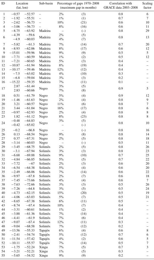
Table 1. Characteristics of the in-situ river level stations: location (latitude, longitude), name of the sub-basin, percentage of gaps in the record over 1980–2008 and maximum of consecutive months missing in the record (in the brackets, “–” means that no month is missing). Correlation GRACE-based TWS data over 2003-2008 (SL>99%) and corresponding scaling factor. We average three pairs of in situ stations (ID: 6, 17 and 24) because these stations are in the same 1◦×1◦GRACE pixel.
ID Location Sub-basin Percentage of gaps 1970–2008 Correlation with Scaling (lat, lon) (maximum gap in months) GRACE data 2003–2008 factor
1 −0.57 −52.57 – 2% (3) 0.8 6
2 −1.92 −55.51 – 1% (1) 0.7 7
3 −2.62 −56.73 – 10% (21) 0.6 10
4 −3.06 −56.73 – 8% (16) 0.6 11
5 −8.75 −63.92 Madeira – (–) 0.8 29
6 −4.39 −59.6 Madeira 2% (5) 0.8 13
−4.9 −60.03 4% (7)
7 −5.82 −61.3 Madeira 7% (14) 0.7 20
8 −8.93 −62.06 Madeira 8% (17) 0.6 12
9 −15.01 −59.96 Madeira 9% (9) 0.5 5
10 −7.71 −60.59 Madeira 1% (2) 0.5 12
11 −7.21 −60.65 Madeira 5% (3) 0.4 –
12 −10.87 −61.94 Madeira 8% (19) 0.4 –
13 −10.17 −59.46 Madeira 12% (12) 0.4 –
14 −7.5 −63.02 Madeira 4% (10) 0.3 –
15 −6.8 −59.04 Madeira 3% (3) 0.2 –
16 −15.22 −59.35 Madeira 7% (11) 0.1 –
17 2.872.83 −−61.4460.66 Negro 3%7% (5)(8) 0.9 5
18 0.51 −61.79 Negro 5% (4) 0.9 12
19 −1.46 −61.63 Negro 2% (4) 0.8 9
20 3.21 −60.57 Negro 11% (6) 0.8 7
21 3.44 −61.04 Negro 16% (17) 0.8 6
22 −0.97 −62.93 Negro 2% (4) 0.8 8
23 1.82 −61.12 Negro 8% (23) 0.8 8
24 −−0.420.48 −−65.0264.83 Negro 3%– (5)(–) 0.8 10
25 −0.2 −66.8 Negro – (–) 0.8 16
26 0.13 −68.54 Negro 9% (8) 0.8 14
27 0.37 −67.31 Negro 2% (5) 0.8 18
28 −3.14 −60.03 Negro – (–) 0.5 11
29 −3.45 −68.75 Solim˜os 2% (5) 0.8 26
30 −3.1 −67.94 Solim˜os 3% (3) 0.8 23
31 −6.68 −69.88 Solim˜os 9% (10) 0.7 25
32 −4.84 −66.85 Solim˜os 5% (5) 0.7 22
33 −7.72 −67 Solim˜os 2% (3) 0.6 20
34 −6.54 −64.38 Solim˜os 5% (4) 0.6 20
35 −2.49 −66.06 Solim˜os 7% (14) 0.6 22
36 −9.97 −67.8 Solim˜os 2% (7) 0.6 18
37 −7.45 −73.66 Solim˜os 4% (4) 0.6 7
38 −7.63 −72.66 Solim˜os 3% (3) 0.5 26
39 −7.26 −64.8 Solim˜os 3% (5) 0.5 24
40 −4.73 −62.15 Solim˜os 15% (20) 0.5 19
41 −4.06 −63.03 Solim˜os 5% (7) 0.5 21
42 −8.65 −67.38 Solim˜os 6% (11) 0.5 –
43 −8.74 −67.4 Solim˜os 10% (7) 0.4 –
44 −3.31 −60.61 Solim˜os 1% (2) 0.4 –
45 −3.88 −61.36 Solim˜os 7% (14) 0.4 –
46 −4.41 −61.9 Solim˜os 7% (6) 0.4 –
47 −9.07 −67.4 Solim˜os 12% (11) 0.3 –
48 −9.04 −68.58 Solim˜os 7% (12) 0.2 –
49 −13.56 −55.33 Tapaj´os 6% (4) 0.6 8
50 −2.41 −54.74 Tapaj´os 5% (12) 0.7 6
51 −11.54 −57.42 Tapaj´os 4% (2) 0.6 5
52 −10.11 −55.57 Tapaj´os 7% (14) 0.5 7
53 −1.75 −52.24 Xingu 7% (5) 0.7 3
54 −3.21 −52.21 Xingu 1% (5) 0.3 –
Laser Retro Reflector. The GRACE Science Data System uses measured inter-satellite range and range rate data, along with ancillary data, to estimate monthly (or sometimes sub-monthly) time series of global Earth’s gravity fields (Bettad-pur, 2007; Flechtner, 2007).
Time variable GRACE global gravity solutions are pro-vided by three GRACE data processing centers of the Sci-ence Data System (SDS): Center for Space Research (CSR) at the University of Texas at Austin, the Geoforschungszen-trum (GFZ) in Potsdam, and the NASA Jet Propulsion Lab-oratory (JPL). The GRACE solutions are distributed by NASA PODAAC (http://podaac.jpl.nasa.gov/grace/). Other groups external to SDS also provide GRACE solutions, e.g., the Goddard Space Flight Center (NASA; Rowlands et al., 2002), the Delft Institute of Earth Observation and Space Systems (DEOS; Klees et al., 2008), the Groupe de Recherche de Geodesie Spatiale (GRGS; Lemoine et al., 2007), among others. The GRACE monthly (or sub monthly) solutions are generally expressed in the form of spherical harmonic coefficients of the geoid height, up to some max-imum degree (typically between 60 and 100, corresponding to wavelengths of∼400 to 700 km). Gridded time series are also available, in general expressed in terms of EWH. Since the beginning of the mission, different GRACE solutions re-leases have been made available by the SDS groups, with im-proved quality from release to release. Here we use GRACE products (release 2) computed by the Groupe de Recherche de Geodesie Spatiale – GRGS (Bruisma et al., 2009). These are monthly EWH solutions provided as 1◦×
1◦
global grids from January 2003 through December 2008. As we focus here on interannual to multidecadal time scales, we removed the seasonal cycle from the gridded GRACE EWH by fitting sinusoids with periods of 12 and 6 months at each grid mesh. We selected GRACE-based EWH data over the Amazon Basin. For small basins, it is necessary to correct for a leak-age factor (due to gravitational signal from outside the con-sidered basin; Chambers, 2006). However over the Amazon Basin, the leakage correction is ∼5% of the seasonal sig-nal (Chen et al., 2007; Ramillien et al., 2008; Xavier et al., 2010). To confirm this result, we estimated the leakage er-ror on the Amazon Basin following Klees et al. (2007) and Longuevergne et al. (2009). Outputs from the Global Land Data Assimilation System (GLDAS-NOAH) (Rodell et al., 2004) has been considered as an a-priori information to com-pute the leakage error over the period 2003–2008. We obtain a leakage error of about 5% of the seasonal cycle, as in pre-vious studies, and around 3% of the interannual signal. As we focus here on the interannual variability, we conclude that the leakage error is negligible.
Figure 2 shows the first three leading modes of the Empir-ical Orthogonal Function (EOF) decomposition (Preisendor-fer, 1988) of gridded TWS based on GRGS GRACE data over 2003-2008. The EOF mode 1 is dominated by a strong positive signal affecting the Negro subbasin and a small area in the southern part of the basin. The EOF mode 2 suggests
Fig. 2. EOF analysis of TWS from GRACE data over 2003– 2008. Spatial patterns of the EOF decomposition of TWS. The three modes are arranged from top to bottom. The principal components are given in the right.
that the Amazon Basin is divided into two main hydrological zones (west and east). The EOF mode 3 shows the mid-2005 drought that affected the centre and the western part of the basin (Chen et al., 2009). These EOF results are very similar to those obtained by Xavier et al. (2010), who made an EOF decomposition of TWS from the CSR GRACE solutions fil-tered by Chambers (2006).
3 Relationship between GRACE-based TWS and in situ river levels
River, and in the Madeira and Negro sub basins, in particular at interannual time scale.
We computed the regression function between in situ river level and GRACE-based EWH time series (annual cycle re-moved), averaging all in situ river level records available in each 1◦
×1◦
GRACE pixel (in order to not weight over pix-els that contain more than one in situ station). The actual GRACE resolution is closer to∼300 km (e.g., Schmidt et al., 2008) but tests made by averaging the in situ data in grid mesh of 3◦×
3◦
did not show significant difference in the reconstruction results. Computing the regression slope be-tween the two data sets is equivalent to computing the ra-tio (called scaling factor) between the standard deviara-tions of both river level and GRACE EWH time series (after remov-ing their mean). The correlations and the scalremov-ing factors for each of 55 in-situ river level stations are gathered in Table 1 (see Fig. 1 for their location). Figure 3 shows in situ water level and GRACE EWH for a subset of 16 sites, chosen for their wide distribution across the basin (note that when 3 sites are located inside a single 1◦
1◦
GRACE mesh, only mean lo-cation and mean river level time series are shown in Fig. 3; in these plots, river level time series are expressed in EWH us-ing the computed scalus-ing factor over span 2003–2008). From Table 1 and Fig. 3, we observe significant correlation on in-terannual time scale between the two data sets (river level and total TWS) at a given location. We also checked that the time series of the EOF decomposition of both GRACE and gauges are consistent over the GRACE period (not shown here).
Using the scaling factor computed over the validation period 2003–2008, TWS virtual records were then recon-structed backward in time (back to 1980) from the river level time series. In the reconstruction we only use in situ river lev-els that do verify a correlation higher than 0.7 with the clos-est GRACE data point. Only 23 sites verify the correlation among a total of 55. This may result from a different hydro-dynamic behaviour between total water storage and surface waters (possibly because of the presence of seasonal flood-plains; Alsdorf et al., 2000; or confluence with a tributary). In situ virtual TWS records used to reconstruct the past 2-D TWS fields will have in common that they are dominated by their surface water component variability. For the Negro sub-basin Frappart et al. (2008) confirmed that the surface water component is not negligible in the interannual TWS, which is almost equally partitioned between surface water and the combination of soil moisture and groundwater. We cannot exclude that in other regions of the Amazon Basin, the rela-tionship does not hold. At first sight, this could bias the re-construction process. Actually this is not the case, as we will see below (see method in Sect. 4) since the functions (EOFs) used to interpolate the virtual records in the reconstruction process are statistical modes of the total TWS variability that intrinsically take into account the co-variability of the dif-ferent layers of the soil at difdif-ferent places (the method op-timally interpolates virtual TWS records that are all domi-nated by their surface waters). In other (not correlated) areas,
reconstructed spatial patterns will be based on the statistical information contained in GRACE TWS grids (provided that these patterns are stationary; see discussion below).
4 Method
The method used to reconstruct past (over 1980–2008) TWS in 2-dimension over the Amazon Basin is based on the re-duced optimal interpolation described by Kaplan et al. (2000) and used by Church et al. (2004) to reconstruct past sea level. This method has 2 steps. In the first step an EOF decomposi-tion (Preisendorfer, 1988; Toumazou and Cretaux, 2001) of the GRACE-based TWS grids is done. This decomposition allows to separate the GRACE signal (here represented by a matrixH, withmlines for each spatial point and n columns for each date) into spatial modes (EOFs) and their related temporal amplitude as follow:,
H(x,y,t ) = U (x,y) α(t ). (2) In this equationU (x,y)stands for the spatial modes andα(t )
for their amplitude over the GRACE period. Assuming that the spatial modesU (x,y)are stationary in time, we deduce that the reconstructed TWS field of the Amazon Basin over the long period 1980–2008 (called hereHR(x,y,t )) has an EOF as follow:
HR(x,y,t ) = U (x,y) αR(t ). (3) whereαR(t )represents the new amplitudes of the EOFs over 1980–2008.
The second step consists of computing the new amplitudes
αR(t )over the whole period 1980–2008 thanks to the in situ virtual TWS records. It is done through a least squares op-timal procedure that minimizes the difference between the reconstructed field and the in situ virtual TWS records at the in situ gauge locations.
In the first step, the EOF modes and amplitudes of the GRACE data set matrixHare computed through a singular value decomposition approach, such that:
H = USVT (4)
whereU (x,y)still stands for the EOF spatial modes, Sis a diagonal matrix containing the singular values ofH and
V represents the temporal eigen modes. At this stage the amplitude α(t ) of the EOF modes can be simply written asα(t )=SVT. Conceptually, each EOFk (k-th column of
is dominated by its surface water component, then for each EOFk, the signalUk(xs, ys)will also be dominated by the surface water. But at the same time, for other points(xj, yj) where this is not the case, thenUk(xj, yj)will carry vari-ability from other layers. TheUk(x,y)modes intrinsically take into account the co-variability of the different layers of the soil at different locations.
The low-order EOFs (eigenvectors of the largest singular values) explain most of the variance and contain the largest spatial scales of the signal. The higher-order EOFs contain smaller spatial scale patterns and are increasingly affected by noise. Besides, their amplitude is decreasingly well re-solved by the least squares procedure because the sparseness of the set of in situ gauges does not allow to resolve too small scale patterns. Consequently, to be efficient, the TWS recon-struction over the Amazon Basin uses only a subset of theM
lowest-order EOFs (the best fit between maximum variance explained and minimum noise perturbation led us to choose
M= 3, which accounts for 79% of the total variance of the GRACE data).
Consequently; the data matrixHcan be written as HM =UM(x, y)α(t ) (5) whereα(t )=SMVT
M is the matrix of the amplitude of theM lowest EOFs. Following Kaplan et al. (2000), in the second step, we compute, at each time step over the time span of the in situ records, the amplitudesαR(t )by minimizing the cost function:
S(α) =
PUM α−H0 T
R−1PUMα −H0
(6) +αT 3−1α
In Eq. (6)H0is the in situ observed TWS,Pis a projection matrix equal to 1 when and where in situ records are available and 0 otherwise and3is a diagonal matrix of theMlargest eigenvalues of the covariance matrix. Ris the error covari-ance matrix accounting for the data error covaricovari-ance matrix (instrumental error) and the error due to the truncation of the set of EOFs to only the firstM EOFs. The second term on the right hand side of the function is a constraint on the EOF spectrum of the solution. It prevents the least squares pro-cedure to be contaminated by high-frequency noise (it filters out non significant solutions that display too much variance at grid points without nearby observations). The least squares procedure is then applied to the virtual in situ TWS records (H0) deduced from the in situ water level records. It provides the reconstructed amplitudeαRof the EOFs.
Since virtual TWS records are all relative to their own lo-cal datum that are not cross-referenced over the basin, this solution may be polluted by spatial variability of the in situ TWS reference surface not necessarily consistent with the GRACE TWS reference surface. To cope with this prob-lem we solved Eq. (3) for changes in TWS between adja-cent steps following Church et al. (2004). Once changes in
amplitude have been obtained at each time step, the ampli-tudes themselves have been recovered integrating backward in time. The integration constants are chosen to equal the re-constructed EOF amplitudes mean to the GRACE EOF am-plitude mean over the GRACE measurement period, ensuring consistency between both sets of EOFs. Finally the recon-structed field of TWS over the Amazonian Basin is obtained by multiplying the first three EOFs with their reconstructed amplitude:
HR = UM(x, y) αR(t ) (7)
5 Stationarity of the spatial patterns
Since the spatial structure of EOFs is sensitive to noise in the observational dataset, we use the longest GRACE dataset available. The GRACE record used in this study spans only 6 years between January 2003 and December 2008 (this is somewhat less but not significantly different from the 9 years of TOPEX/Poseidon altimetry data used by Church et al., 2004, to reconstruct past 50 years sea level). However, as full coverage of the Amazon Basin’s TWS is only available for the GRACE period, there is no other way to determine TWS spatial patterns. As an alternative, EOFs could have been computed from long hydrological model outputs. But while hydrological models agree rather well in terms of TWS spatial average, they much differ when looking at the spatial patterns.
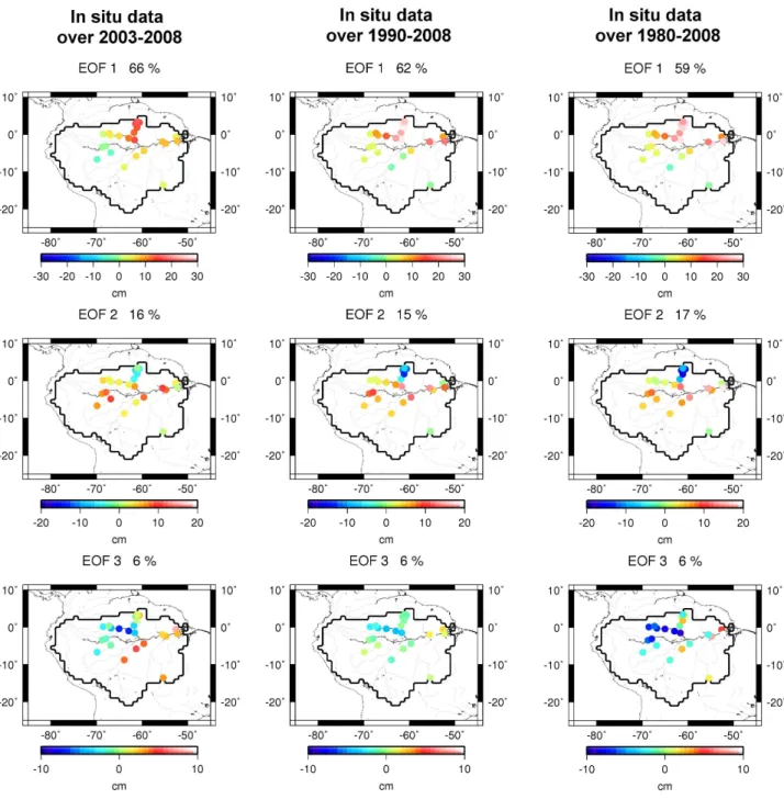
One possible drawback of using GRACE to compute spa-tial EOFs is linked to the question of (non) stationarity in time of the spatial patterns. Here, we assume that the EOF spatial patterns of the GRACE TWS capture most of the in-terannual/decadal variability. To test this stationary assump-tion (inherent to the method used here), we consider a dataset composed of 23 in situ gauges (black dots in Fig. 4, see be-low), spanning over the period 1980–2008. We computed the river level EOFs over three interval subsets (2003–2008, 1990–2008 and 1980–2008). Corresponding first 3 leading modes (>80% of the total variance) are shown in Fig. 4. Very little difference is noticed between the three cases. It is strik-ing to see how the EOFs are similar despite the different time span over which they have been computed.
Fig. 4.Spatial patterns of the third EOFs computed from in situ gauges. The black dots correspond to the 23 in situ gauges (the same 23 used in the reconstruction) used for the EOF analysis over 2003–2008 (left panel), 1990–2008 (middle panel) and over 1980–2008 (right panel).
We conclude that surface water patterns (hence TWS fields, because of the reported correlation) and precipitation pat-terns are quasi stationary with time (at least as far as the early 1980s). Thus the basic assumption of our reconstruc-tion method (stareconstruc-tionarity of the spatial EOFs) holds.
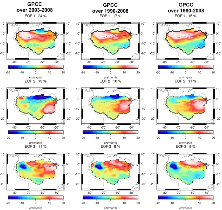
Fig. 5.Spatial patterns of the third EOFs computed from GPCC. EOF analysis over 2003–2008 (left panel), 1990–2008 (middle panel) and over 1980–2008 (right panel).
6.1 Reconstructed TWSR averaged over the Amazon Basin
Figure 6 shows past TWSR (1980–2008) averaged over the Amazon Basin (a 5-month smoothing was applied to the time series; TWSR holds for reconstructed TWS). For com-parison, we also show the reconstructed TWSR (with same smoothing) over 1990–2008. For the latter case, a larger number (36) of in situ stations well correlated (r >0.7) with GRACE TWS were available. Hence a larger number of vir-tual TWS time series could be used. Comparing the two re-constructions shows very little difference, suggesting that the
number of virtual stations is not critical, provided that they are well distributed across the basin (see Fig. 1). In Fig. 6 is also shown GRACE-based mean TWS, which superimposes well with the reconstructed curves.
Fig. 6.Basin-averaged of the TWSR. The basin-averaged of the TWSR over 1980–2008 is the black line. The basin-averaged of the TWSR over 1990–2008 is the red line. The TWS GRACE data is superimposed in dot line over 2003–2008. We filtered out the high frequencies using a simple 5-month running mean.ris the correlation coefficient (with a significance level higher than 99%).
Fig. 7.Basin-averaged of the TWSR comparison with ISBA-TRIP. The basin-averaged of the TWSR is the black line and its error bars are in grey. The error in TWSR computed here is the sum of the error due to the least squares method and the error of the in situ records. This signal accounts for 60% of the total reconstructed signal variance. ISBA-TRIP is in red line. The El Ni˜no events are represented by arrows. We filtered out the high frequencies (>1 yr−1) using a simple 12-month running mean. ris the correlation coefficient (with a significance level higher than 99%).
soil depth. Several surface water storage compartments as dams, lakes, or groundwater storage are not simulated in the ISBA-TRIP model. The soil water content varies with surface infiltration, soil evaporation, plant transpiration and deep drainage. The infiltration rate is computed as the dif-ference between the through-fall rate and the surface runoff. The through-fall rate is the sum of rainfall not intercepted by the canopy, dripping from the interception reservoir and snowmelt from the snow pack. ISBA also uses a compre-hensive parameterization of sub-grid hydrology to account for the heterogeneity of precipitation, topography and vege-tation within each grid cell (Decharme and Douville, 2007). TRIP -Total Runoff Integrating Pathways- was developed by Oki and Sud (1998). It is a simple runoff routine model used to convert the daily runoff simulated by 1◦
by 1◦
resolution. The ISBA-TRIP version used in this study is driven by pre-scribed atmospheric forcing using monthly precipitation data from the Global Precipitation Climatology Center (GPCC) Full Data Product V4 (Alkama et al., 2010; Decharme et al., 2010). The temporal resolution of this data set in 1 month.
in ISBA-TRIP could explain the small differences that re-main between the two curves. We observe TWS minima during ENSO events (indicated by arrows in Fig. 7), as ex-pected from previously reported correlation between ENSO and rainfall and in situ discharge data over the Amazon Basin (Marengo, 2004; Molinier et al., 2009; Ronchail et al., 2002). The lack of trend in both curves (reconstruction and ISBA-TRIP model) suggests no net gain or loss in total water stor-age over the Amazonian Basin between 1980 and 2008.
In Fig. 7, the grey zone represents uncertainty in TWSR. This uncertainty is based on the sum of errors due to the least-squares inversion (as presented in Sect. 4) and errors of the in situ records. This latter error is estimated from a bootstrap method for standard errors of the in situ water lev-els for each month (significant at the 95% level). Actually, the reconstruction method includes additional uncertainties. For example, the scaling factor between in situ river level and GRACE-based TWS may introduce some uncertainty. Indeed, river level may be more closely tied to the surface wetness condition than to groundwater (or TWS). Another source of error possibly be due to precipitation events in up-stream areas, may affect downup-stream water levels with some time delay due to water transport. GRACE measurements have also their own uncertainty. As a matter of fact, GRACE-based TWS is not a point measurement (as it is the case for river level) but represents an average over a much larger re-gion (of about 300 km size). All these uncertainties will af-fect the precision of the reconstruction but they are very dif-ficult to estimate. They have been neglected here. Thus the grey zone likely underestimates of the actual uncertainty. 6.2 Spatial patterns of TWSR
We have analysed the spatial patterns of the 2-D TWSR fields over 1980–2008 and 1990–2008, through an EOF decompo-sition approach. Results are shown in Fig. 8. The spatially constant mode (EOF0, around 60% of the total variance for each TWSR) which represents the interannual variability of the mean TWSR over the Amazon Basin from 1980–2008 is that shown in Figs. 6 and 7.
Figure 8 shows the first three EOF modes of the TWSR fields over the two time spans (1990–2008 and 1980–2008). Recall that the 1990–2008 reconstruction is based on a larger set of in situ station than the 1980–2008 one (36 versus 23). Looking at the spatial pattern maps and at the temporal curves, we note quite good agreement between the two re-constructions (1990–2008 and 1980–2008), as previously noticed for the mean TWSR. On EOF1 (26% and 25% of the total variance) temporal curve, we have superimposed the Southern Oscillation Index (SOI; mean sea-level pressure difference between Tahiti and Darwin), a proxy of ENSO. Correlation between SOI and TWS mode 1 is high (r= 0.7 with a SL>99%). In the north-eastern region, including the Negro sub-basin, and in the Madeira basin, where EOF1 ex-hibits a strong positive anomaly in the spatial map, minima
in local TWS correspond to negative SOI (warm phase of ENSO). In contrast, a negative correlation can be observed locally between SOI and TWS mode 1 in the Tapajos and the Xingu sub-basins. Studies have shown that precipitation over the northeastern part of the Amazon Basin is largely controlled by ENSO (Zeng, 1999; Marengo, 1992; Espinoza et al., 2009). Thus, a positive correlation between mean TWS and SOI is expected, as our result indeed shows.
Studies provided diagnostic evidence of ENSO low fre-quency modulation (McCabe and Dettinger, 1999; Gutzler et al., 2002), in particular by the Pacific Decadal Oscilla-tion (PDO) (Mantua et al., 1997). The PDO index is de-fined as the leading principal component of the North Pacific monthly sea surface temperature variability. The PDO is a long-lived El Ni˜no–like pattern of Pacific climate variability. In the cool (warm) phases of PDO, the central and northwest Pacific sea surface temperature (SST) is warm (cold) and the SST at the coast of the North America is of cold (warm) SST. In Fig. 8, is displayed the EOF2 temporal curve of TWS with the PDO index superimposed. Correlation between PDO and TWS EOF2 is significant (r=−0.5 with a SL >99%). In the whole eastern Amazon Basin, where the spatial EOF2 mode shows a negative pattern, local TWSR temporal vari-ability is negatively correlated to the PDO index, while in the Negro and the Solim˜oes sub-basins a positive correlation is observed.
The spatial pattern and temporal curve of the EOF3 in Fig. 8 reflect the recurrent droughts that affect the centre of the Amazon Basin, in particular the main river. These are indicated by arrows on the temporal curve. The well publi-cized 2005 drought is clearly visible. It has been reported to be one of the most intense droughts of the past 100 years in the Amazon Basin (Marengo et al., 2008; Zeng et al., 2008; Chen et al., 2009), but the TWSR mode 3 seems to indicate that the 1980 and 1998 droughts had even stronger impact in terms of basin total water storage depletion. Drought events in 1983 and 1998 occurred during El Ni˜no years, unlike in 1980, 1992, 1995 and 2005.
7 Conclusions
Fig. 8. EOF analysis of TWSR. The left panel shows the EOF analysis for the TWSR over 1990–2008. The locations of the 36 in situ stations used for the reconstruction are indicated by black dots. The right panel shows the EOF analysis for the TWSR over 1980–2008. The locations of the 23 in situ stations used for the reconstruction are indicated by black dots. The middle panel shows the EOFs’ time series computed on the TWSR over 1990–2008 in red line and in black line over 1980–2008, and superimposed(a)the scaled SOI index (dash line) and the El Ni˜no events (arrows),(b)the inverse scaled PDO index (dash line) and(c)the drought events (arrows). We filter out the high frequencies (>1 yr−1) using a simple 12-month running mean.
The observed timing and regional distribution of the TWSR over the Amazonian Basin during∼30 years shows no long-term trend and confirms the dominant influence of ENSO and PDO. In addition, recurrent drought events af-fecting the centre of the basin are also well reproduced. The approach developed in this study offers interesting perspec-tive for improving our knowledge of past TWS in many river basins over the world where climate variability is the main driver of TWS change. However, it will be less easily ap-plicable in river basins which have been strongly affected by anthropogenic forcing over the GRACE period, such as in northern India. Indeed, in these basins, GRACE measure-ment may be impacted by the recent ground water mining used for crop irrigation (Rodell et al., 2009; Tiwari et al.,
Acknowledgements. M. Becker and R. Alkama were supported by the CYMENT project of the RTRA “Sciences et Technologies pour l’A´eronautique et l’Espace” STAE. L. Xavier has been supported by a grant of Brazilian agency CAPES (Coordenac¸˜ao de Aperfeic¸oamento de Pessoal de N´ıvel Superior).
Edited by: J. Liu
The publication of this article is financed by CNRS-INSU.
References
Alkama, R., Decharme, B., Douville, H., Becker, M., Cazenave, A., Sheffield, J., Voldoire, A., Tyteca, S., and Le Moigne, P.: Global evaluation of the ISBA-TRIP continental hydrologic sys-tem, Part 1: a two-fold constraint using GRACE terrestrial water storage estimates and in situ river discharges, J. Hydrometeorol., 11, 583 - 600, 2010.
Alsdorf, D. E., Melack, J. M., Dunne, T., Mertes, L. A. K., Hess, L. L., and Smith, L. C.: Interferometric radar measurements of water level changes on the Amazon floodplain, Nature, 404, 174– 177, 2000.
Alsdorf, D. E., Rodriguez, E., and Lettenmaier, D. P.: Measuring surface water from space, Rev. Geophys., 45, 1–24, 2007. Bettadpur, S.: CSR Level-2 Processing Standards Document for
Product Release 04, GRACE 327-742, The GRACE Project, Center for Space Research, University of Texas at Austin, 2007. Bruinsma, S., Lemoine, J.-M., Biancale, R., and Vales, N.: CNES/GRGS 10-day gravity field models (release 2) and their evaluation, Adv. Space Res., 45, 587–601, 2009.
Calafat, F. M. and Gomis, D.: Reconstruction of Mediterranean sea level fields for the period 1945–2000, Global Planet. Change, 66, 225–235, 2009.
Chambers, D. P.: Evaluation of new GRACE time-variable grav-ity data over the ocean, Geophys. Res. Lett., 33, L17603, doi:10.1029/2006GL027296, 2006.
Chambers, D. P., Mehlhaff, C. A., Urban, T. J., Fujii, D., and Nerem, R.: S. Low-frequency variations in global mean sea level: 1950–2000, J. Geophys. Res., 107, 3026, 2002.
Chen, J. L., Wilson, C. R., Famiglietti, J. S., and Rodell, M.: Atten-uation Effects on Seasonal Basin-Scale Water Storage Change From GRACE Time-Variable Gravity, J. Geodesy, 81(4), 237– 245, doi:10.1007/s00190-006-0104-2, 2007.
Chen, J. L., Wilson, C. R., Tapley, B. D., Yang, Z. L., and Niu, G. Y.: 2005 drought event in the Amazon River basin as measured by GRACE and estimated by climate models, J. Geophys. Res., 114, B05404, doi:10.1029/2008JB006056, 2009.
Church, J. A., White, N. J., Coleman, R., Lambeck, K., and Mitro-vica, J. X.: Estimates of the regional distribution of sea level rise over the 1950–2000 period, J. Climate, 17, 2609–2625, 2004.
Clarke, R. T.: Uncertainty in the estimation of mean annual flood due to rating-curve in definition, J. Hydrol., 22(1–4), 185–190, doi:10.1016/S0022-1694(99)00097-9, 1999.
Decharme, B. and Douville, H.: Global validation of the ISBA sub-grid hydrology, Clim. Dynam., 29, 21–37, 2007.
Decharme, B., Alkama, R., Douville, H., Becker, M., and Cazenave, A.: Global Evaluation of the ISBA-TRIP Continental Hydrolog-ical System, Part II: Uncertainties in River Routing Simulation Related to Flow Velocity and Groundwater Storage, J. Hydrom-eteorol., 11, 601–617, 2010.
D¨oll, P., Kaspar, F., and Lehner, B.: A global hydrological model for deriving water availability indicators: model tuning and vali-dation, J. Hydrol., 270, 105–134, 2003.
Espinoza Villar, J. C., Ronchail, J., Guyot, J. L., Cochonneau, G., Naziano, F., Lavado, W., De Oliveira, E., Pombosa, R., and Vauchel, P.: Spatio-temporal rainfall variability in the Amazon basin countries (Brazil, Peru, Bolivia, Colombia, and Ecuador), Int. J. Climatol., 29(11), 1574–1594, 2009.
Flechtner, F.: GFZ Level-2 Processing Standards Document for Product Release 04, GRACE, Department 1: Geodesy and Remote Sensing, GeoForschungszentrum Potsdam, Flechtner, 2007.
Frappart, F., Papa, F., Famiglietti, J. S., Prigent, C., Rossow, W. B., and Seyler, F.: Interannual variations of river water storage from a multiple satellite approach: A case study for the Rio Negro River basin, J. Geophys. Res., 113, D21104, doi:10.1029/2007JD009438, 2008.
Gutzler, D. S., Kann, D. M., and Thornbrugh, C.: Modulation of ENSO-based long-lead outlooks of southwestern US winter pre-cipitation by the Pacific Decadal Oscillation, Weather Forecast., 17, 1163–1172, 2002.
Kaplan, A., Kushnir, Y., and Cane, M. A.: Reduced space optimal interpolation of historical marine sea level pressure: 1854–1992, J. Climate, 13, 2987–3002, 2000.
Klees, R., Zapreeva, E. A., Winsemius, H. C., and Savenije, H. H. G.: The bias in GRACE estimates of continental wa-ter storage variations, Hydrol. Earth Syst. Sci., 11, 1227–1241, doi:10.5194/hess-11-1227-2007, 2007.
Klees, R., Liu, X., Wittwer, T., Gunter, B. C., Revtova, E. A., Tenze, R., Ditmar, P., Winsemius, H. C., and Savenije, H. H. G.: A com-parison of global and regional GRACE models for land hydrol-ogy, Surv. Geophys., 29, 335–359, 2008.
Lemoine, J. M., Bruinsma, S., Loyer, S., Biancale, R., Marty, J. C., Perosanz, F., and Balmino, G.: Temporal gravity field models in-ferred from GRACE data, Adv. Space Res., 39(10), 1620–1629, 2007.
Liu, J. and Yang H.: Spatially explicit assessment of global con-sumptive water uses in cropland: green and blue water, J. Hy-drol., 384, 187–197, 2010.
Liu, J., Zehnder, A. J. B., and Yang, H.: Global consump-tive water use for crop production: The importance of green water and virtual water, Water Resour. Res., 45, W05428, doi:10.1029/2007WR006051, 2009.
Longuevergne, L., Scanlon, B. R., and Wilson, C. R.: GRACE Hy-drological estimates for small basins: Evaluating processing ap-proaches on the High Plains Aquifer, USA, Water Resour. Res., 46, W11517, doi:10.1029/2009WR008564, 2010.
Mantua, N. J., Hare, S. R., Zhang, Y., Wallace, J. M., and Francis, R. C.: A Pacific interdecadal climate oscillation with impacts on salmon production, B. Am. Meteorol. Soc., 78, 1069–1079, 1997.
Marengo, J. A.: Interannual variability of surface climate in the Amazon basin, Int. J. Climatol., 12, 853–863, 1992.
Marengo, J. A.: Interdecadal variability and trends of rainfall across the Amazon basin, Theor. Appl. Climatol., 78, 79–96, 2004. Marengo, J. A., Nobre, C. A., Tomasella, J., Oyama, M. D.,
Sam-paio de Oliveira, G., de Oliveira, R., Camargo, H., Alves, L. M., and Brown, I. F.: The drought of Amazonia in 2005, J. Climate, 21, 495–516, 2008.
Masuda, K., Hashimoto, Y., Matsuyama, H., and Oki, T.: Seasonal cycle of water storage in major river basins of the world, Geo-phys. Res. Lett., 28, 3215–3218, 2001.
McCabe, G. J. and Dettinger, M. D.: Decadal variations in the strength of ENSO teleconnections with precipitation in the west-ern United States, Int. J. Climatol., 19, 1399–1410, 1999. Milly, P. C. D. and Shmakin, A. B.: Global modeling of land water
and energy balances, Part I: The Land Dynamics (LaD) model, J. Hydrometeorol., 3, 283–299, 2002.
Molinier, M., Ronchail, J., Guyot, J. L., Cochonneau, G., Guimaraes, V., and de Oliveira, E.: Hydrological variability in the Amazon drainage basin and African tropical basins, Hydrol. Process., 23, 3245–3252, 2009.
Noilhan, J. and Planton, S.: A simple parameterization of land sur-face processes for meteorological models, Mon. Weather Rev., 117, 536–549, 1989.
Oki, T. and Sud, Y.: Design of the global river channel network for Total Runoff Integrating Pathways (TRIP), Earth Interact., 2, 1–36, 1998.
Preisendorfer, R. W.: Principal Component Analysis in Meteorol-ogy and Oceanography, New York, 1–455, 1988.
Ramillien, G., Bouhours, S., Lombard, A., Cazenave, A., Flecht-ner, F., and Schmidt, R.: Land water storage contribution to sea level from GRACE geoid data over 2003–2006, Global Planet. Change, 60, 381–392, doi:10.1016/j.gloplacha.2007.04.002, 2008.
Rodell, M. and Famiglietti, J. S.: Detectability of variations in con-tinental water storage from satellite observations of the time de-pendent gravity field, Water Resour. Res. 35, 2705–2724, 1999. Rodell, M., Houser, P. R., Jambor, U., Gottschalck, J., Mitchell,
K., Meng, C. J., Arsenault, K., Cosgrove, B., Radakovich, J., and Bosilovich, M.: The global land data assimilation system, B. Am. Meteorol. Soc., 85, 381–394, 2004.
Rodell, M., Velicogna, I., and Famiglietti, J. S.: Satellite-based esti-mates of groundwater depletion in India, Nature, 460, 999–1002, 2009.
Ronchail, J., Cochonneau, G., Moloinier, M., Guyot, J. L., Goretti de Miranda Chaves, A., Guimaraes, V., and De Oliveira, E.: In-terannual rainfall variability in the Amazon basin and sea-surface temperatures in the equatorial Pacific and the tropical Atlantic Oceans, Int. J. Climatol., 22, 1663–1686, 2002.
Rosner, B.: On the detection of many outliers, Technometrics, 17, 221–227, 1975.
Rowlands, D. D., Ray, R. D., Chinn, D. S., and Lemoine, F. G.: Short-arc analysis of intersatellite tracking data in a gravity map-ping mission, J. Geodesy, 76, 307–316, 2002.
Rudolf, B.: The Global Precipitation Climatology Centre, WMO Bull., 44, 77–78, 1995.
Schmidt, R., Flechtner, F., Meyer, U., Neumayer, K. H., Dahle, Ch., Konig, R., and Kushe, J.: Hydrological signals observed by the GRACE satellites, Surv. Geophys., 29, 319–334, 2008. Shiklomanov, A. I., Lammers, R. B., and Vorosmarty, C. J.:
Widespread decline in hydrological monitoring threatens, Pan-Arctic research, EOS Transact. AGU, 83, 13–16, 2002. Smith, T. M. and Reynolds, R. W.: Extended reconstruction of
global sea surface temperatures based on COADS data (1854– 1997), J. Climate, 16, 1495–1510, 2003.
Tapley, B. D., Bettadpur, S., Watkins, M., and Reigber, C.: The gravity recovery and climate experiment: Mission overview and early results, Geophys. Res. Lett., 31, L09607, doi:10.1029/2004GL019920, 2004.
Tiwari, V. M., Wahr, J., and Swenson, S.: Dwindling groundwater resources in northern India, from satellite gravity observations, Geophys. Res. Lett., 36, L18401, doi:10.1029/2009GL039401, 2009.
Toumazou, V. and Cretaux, J. F.: Using a Lanczos eigensolver in the computation of Empirical Orthogonal Functions, Mon. Weather Rev., 129, 1243–1250, 2001.
Vaz De Almeida, F. : Study of the temporal variations of the ter-restrial gravitational field from the GRACE mission data: Appli-cation in the Amazonian basin, Ph.D. thesis, University of S˜ao Paulo, Brazil, 2009.
Wahr, J., Swenson, S., Zlotnicki, V., and Velicogna, I.: Time-variable gravity from GRACE: First results, Geophys. Res. Lett., 31, L11501, doi:10.1029/2004GL019779, 2004.
Xavier, L., Becker, M., Cazenave, A., Longuevergne, L., Llovel, W., and Rotunno Filho, O. C.: Interannual variability in wa-ter storage over 2003–2008 in the Amazon Basin from GRACE space gravimetry, in situ river level and precipitation data, Re-mote Sens. Environ., 114, 1629–1637, 2010.
Zeng, N.: Seasonal cycle and interannual variability in the Ama-zon hydrologic cycle, J. Geophys. Res.-Atmos., 104, 9097–9106, 1999.