Submitted 3 August 2015 Accepted 5 November 2015 Published25 November 2015 Corresponding author
Nuno Fachada, [email protected]
Academic editor
Feng Gu
Additional Information and Declarations can be found on page 24
DOI10.7717/peerj-cs.36 Copyright
2015 Fachada et al.
Distributed under
Creative Commons CC-BY 4.0 OPEN ACCESS
Towards a standard model for research in
agent-based modeling and simulation
Nuno Fachada1, Vitor V. Lopes2, Rui C. Martins3and Agostinho C. Rosa1
1Institute for Systems and Robotics, LARSyS, Instituto Superior T´ecnico, Universidade de Lisboa,
Lisboa, Portugal
2Universidad de las Fuerzas Armadas-ESPE, Sangolqu´ı, Ecuador
3Life and Health Sciences Research Institute, School of Health Sciences, University of Minho,
Braga, Portugal
ABSTRACT
Agent-based modeling (ABM) is a bottom-up modeling approach, where each entity of the system being modeled is uniquely represented as an independent decision-making agent. ABMs are very sensitive to implementation details. Thus, it is very easy to inadvertently introduce changes which modify model dynamics. Such problems usually arise due to the lack of transparency in model descriptions, which constrains how models are assessed, implemented and replicated. In this paper, we present PPHPC, a model which aims to serve as a standard in agent based modeling research, namely, but not limited to, conceptual model specification, statistical analysis of simulation output, model comparison and parallelization studies. This paper focuses on the first two aspects (conceptual model specification and statistical analysis of simulation output), also providing a canonical implementation of PPHPC. The paper serves as a complete reference to the presented model, and can be used as a tutorial for simulation practitioners who wish to improve the way they communicate their ABMs.
Subjects Agents and Multi-Agent Systems, Scientific Computing and Simulation, Theory and Formal Methods
Keywords Agent-based modeling, Standard model, Statistical analysis of simulation output, ODD
INTRODUCTION
Spatial agent-based models (SABMs) are a subset of ABMs in which a spatial topology defines how agents interact (Shook, Wang & Tang, 2013). For example, an agent may be limited to interact with agents located within a specific radius, or may only move to a near physical or geographical location (Macal & North, 2010). SABMs have been extensively used to study a range of phenomena in the biological and social sciences (Isaac, 2011; Shook, Wang & Tang, 2013).
ABMs are very sensitive to implementation details: the impact that seemingly unimportant aspects such as data structures, algorithms, discrete time representation, floating point arithmetic or order of events can have on results is tremendous (Wilensky & Rand, 2007;Merlone, Sonnessa & Terna, 2008). As such, it is very easy to inadvertently introduce changes which will alter model dynamics. These type of issues usually derive from a lack of transparency in model descriptions, which constrains how models are assessed and implemented (M¨uller et al., 2014). Conceptual models should be well specified and adequately described in order to be properly implemented and replicated (Edmonds & Hales, 2003;Wilensky & Rand, 2007).
The ODD protocol (Overview, Design concepts, Details) is currently one of the most widely used templates for making model descriptions more understandable and complete, providing a comprehensive checklist that covers virtually all the key features that can define a model (Grimm et al., 2010). It allows modelers to communicate their models using a natural language description within a prescriptive and hierarchical structure, aiding in model design and fostering in-depth model comprehension (M¨uller et al., 2014). It is the recommended approach for documenting models in the CoMSES Net Computational Model Library (Rollins et al., 2014). However,M¨uller et al. (2014)argue that no single model description standard can completely and throughly characterize a model by itself, suggesting that besides a structured natural language description such as ODD, the availability of a model’s source code should be part of a minimum standard for model communication. Furthermore, the ODD protocol does not deal with models from a results or simulation output perspective, which means that an additional section for statistical analysis of results is often required. In practice, however, the situation is very different. While many ABMs have been published and simulation output analysis is a
widely discussed subject matter (Sargent, 1976;Kelton, 1997;Law, 2007;Nakayama, 2008; Law, 2015), comprehensive inquiries concerning the output of ABM simulations are hard to find in the scientific literature.
In this paper, we present PPHPC (Predator-Prey for High-Performance Computing), a conceptual model which captures important characteristics of SABMs, such as agent movement and local agent interactions. It aims to serve as a standard in agent based modeling research, and was designed with several goals in mind:
1. Provide a basis for a tutorial on complete model specification and thorough simulation output analysis.
3. Compare different implementations from a performance point of view, using different
frameworks, programming languages, hardware and/or parallelization strategies, while maintaining statistical equivalence among implementations (Fachada et al., 2015b). 4. Test the influence of different pseudo-random number generators (PRNGs) on the
statistical accuracy of simulation output.
This paper aims to fulfill the first of these goals, and is organized as follows. First, in ‘Background,’ we review several paradigmatic ABMs, as well as model description and analysis. Next, the ‘Methodology’ section is divided into five subsections, in which we: (a) formalize the conceptual model using the ODD protocol; (b) describe the canonical PPHPC realization implemented with the NetLogo ABM toolkit (Wilensky, 1999); (c) discuss how to select output focal measures; (d) explain how to collect and prepare data for statistical analysis; and, (e) propose how to analyze focal measures from a statistical point-of-view. In ‘Results’, statistical analysis of output of the NetLogo implementation is performed. A discussion on how these results can be utilized in additional investigations is undertaken in ‘Discussion’. ‘Conclusions’ provides a global outline of what was accomplished in this paper.
BACKGROUND
Several ABMs have been used for the purpose of modeling tutorials and/or model analysis and replication. Probably, the most well known standard ABM is the “StupidModel,” which consists of a series of 16 pseudo-models of increasing complexity, ranging from simple moving agents to a full predator-prey-like model. It was developed byRailsback, Lytinen & Grimm (2005)as a teaching tool and template for real applications, as it includes a set of features commonly used in ABMs of real systems. It has been used to address a number of questions, including the comparison of ABM platforms (Railsback, Lytinen & Jackson, 2006;Lytinen & Railsback, 2012), model parallelization (Lysenko & D’Souza, 2008;Tang & Wang, 2009), analysis of toolkit feasibility (Standish, 2008) and/or creating models as compositions of micro-behaviors (Kahn, 2007). The “StupidModel” series has been criticized for having some atypical elements and ambiguities (Lytinen & Railsback, 2012), reasons which leadIsaac (2011)to propose a reformulation to address these and other issues. However, its multiple versions and user-interface/visualization goals limit the series appeal as a pure computational model for the goals described in the introduction.
& Hales, 2003;Wilensky & Rand, 2007). This might not come as a surprise, as most models are not implemented with replication in mind.
Many models are not adequately analyzed with respect to their output data, often due to improper design of simulation experiments. Consequently, authors of such models can be at risk of making incorrect inferences about the system being studied (Law, 2007). A number of papers and books have been published concerning the challenges, pitfalls and opportunities of using simulation models and adequately analyzing simulation output data. In one of the earliest articles on the subject,Sargent (1976)demonstrates how to obtain point estimates and confidence intervals for steady state means of simulation output data using a number of different methodologies. Later,Law (1983)presented
a state-of-the-art survey on statistical analyses for simulation output data, addressing issues such as start-up bias and determination of estimator accuracy. This survey was updated several times over the years, e.g.,Law (2007), where Law discusses the duration of transient periods before steady state settles, as well as the number of replications required for achieving a specific level of estimator confidence. InKelton (1997), the author describes methods to help design the runs for simulation models and interpreting their output using statistical methods, also dealing with related problems such as model comparison, variance reduction or sensitivity estimation. A comprehensive exposition of these and other important topics of simulation research is presented in the several editions of “Simulation Modeling and Analysis” by Law and Kelton, and its latest edition (Law, 2015) is used as a starting point for the analysis described in ‘Methodology’ and conducted in ‘Results.’
METHODOLOGY
Overview, design concepts and details of PPHPC
Here we describe the PPHPC model using the ODD protocol (Grimm et al., 2010). Time-dependent state variables are represented with uppercase letters, while constant state variables and parameters are denoted by lowercase letters. TheU(a,b)expression equates to a random integer within the closed interval[a,b]taken from the uniform distribution.
Purpose
The purpose of PPHPC is to serve as a standard model for studying and evaluating SABM implementation strategies. It is a realization of a predator-prey dynamic system, and captures important characteristics of SABMs, such as agent movement and local agent interactions. The model can be implemented using substantially different approaches
that ensure statistically equivalent qualitative results. Implementations may differ in
Table 1 Model state variables by entity.Where applicable, thesandwdesignations correspond to prey (sheep) and predator (wolf) agent types, respectively.
Entity State variable Symbol Range
Type t s,w
Energy E 1,2,...
Horizontal position in grid X 0,1,...,xenv−1
Vertical position in grid Y 0,1,...,yenv−1
Energy gain from food gs,gw 0,1,...
Energy loss per turn ls,lw 0,1,...
Reproduction threshold rTs,rwT 1,2,...
Agents
Reproduction probability rPs,rPw 0,1,...,100 Horizontal position in grid x 0,1,...,xenv−1
Vertical position in grid y 0,1,...,yenv−1
Grid cells
Countdown C 0,1,...,cr
Horizontal size xenv 1,2,...
Vertical size yenv 1,2,...
Environment
Restart cr 1,2,...
Entities, state variables, scales
The PPHPC model is composed of three entity classes:agents,grid cellsandenvironment. Each of these entity classes is defined by a set of state variables, as shown inTable 1. All state variables explicitly assume integer values to avoid issues with the handling of floating-point arithmetic on different programming languages and/or processor architectures.
Thetstate variable defines theagent type, eithers(sheep, i.e. prey) orw(wolf, i.e. predator). The only behavioral difference between the two types is in the feeding pattern:
while prey consume passive cell-bound food, predators consume prey. Other than that, prey and predators may have different values for other state variables, as denoted by the
superscriptssandw. Agents have an energy state variable,E, which increases bygsorgw
when feeding, decreases bylsorlwwhen moving, and decreases by half when reproducing. When energy reaches zero, the agent is removed from the simulation. Agents with energy higher thanrsTorrTwmay reproduce with probability given byrPs orrPw. The grid position state variables,XandY, indicate which cell the agent is located in. There is no conceptual limit on the number of agents that can exist during the course of a simulation run.
Instances of thegrid cellentity class can be thought of the place or neighborhood where agents act, namely where they try to feed and reproduce. Agents can only interact with other agents and resources located in the same grid cell. Grid cells have a fixed grid position,(x,y), and contain only one resource, cell-bound food (grass), which can be consumed by prey, and is represented by the countdown state variableC. TheCstate variable specifies the number of iterations left for the cell-bound food to become available. Food becomes available whenC=0, and when a prey consumes it,Cis set tocr.
The set of all grid cells forms theenvironmententity, a toroidal square grid where the simulation takes place. The environment is defined by its size,(xenv,yenv), and by the restart
Spatial extent is represented by the aforementioned square grid, of size(xenv,yenv),
wherexenvandyenv are positive integers. Temporal extent is represented by a positive
integerm, which represents the number of discrete simulation steps or iterations. Spatial and temporal scales are merely virtual, i.e. they do not represent any real measure.
Process overview and scheduling
Algorithm 1 describes the simulation schedule and its associated processes. Execution starts with an initialization process,Init(), where a predetermined number of agents are randomly placed in the simulation environment. Cell-bound food is also initialized at this stage.
After initialization, and to get the simulation state at iteration zero, outputs are gathered by theGetStats()process. The scheduler then enters the main simulation loop, where each iteration is sub-divided into four steps: (1) agent movement ; (2) food growth in grid cells; (3) agent actions ; and, (4) gathering of simulation outputs. State variables
Algorithm 1Main simulation algorithm.forloops can be processed inany orderor in
random order. In terms of expected dynamic behavior, the former means the order is not relevant, while the latter specifies loop iterations should be explicitly shuffled.
1: I() 2: GS() 3: i←1
4: fori<=mdo
5: for eachagentdo ◃Any order
6: M() 7: end for
8: for eachgrid celldo ◃Any order
9: GF() 10: end for
11: for eachagentdo ◃Random order
12: A() 13: end for 14: GS() 15: i←i+1 16: end for
are asynchronously updated, i.e. they are assigned a new value as soon as this value is calculated by a process (e.g., when an agent gains energy by feeding).
Design concepts
model can provide valuable information on how to better implement SABMs on different
computing architectures, namely parallel ones. In particular, they may shown the impact of different parallelization strategies on simulation performance.
Emergence. The model is characterized by oscillations in the population of both prey and predator, as well as in the available quantity of cell-bound food. Typically, a peak of predator population occurs slightly after a peak in prey population size, while quantity of cell-bound food is approximately in “phase opposition” with the prey’s population size.
Sensing. Agents can sense the presence of food in the grid cell in which they are currently located. This means different thing for prey and predators. Prey agents can read the local
grid cellCstate variable, which if zero, means there is food available. Predator agents can determine the presence of prey agents.
Interaction. Agents interact with sources of food present in the grid cell they are located in.
Stochasticity. The following processes are random: (a) initialization of specific state variables; (b) agent movement; (c) the order in which agents act; and, (d) agent reproduction.
Observation. The following vector is collected in theGetStats()process, whereirefers to the current iteration:
Oi=(Psi,Piw,Pci,E s i,E
w i ,Ci)
Psi andPwi refer to the total prey and predator population counts, respectively, whilePic
holds the quantity of available cell-bound food.EsiandEwi contain the mean energy of prey and predator populations. Finally,Cirefers to the mean value of theCstate variable in all
grid cells.
Initialization
The initialization process begins by instantiating theenvironmententity, a toroidal square grid, and filling it withxenv×yenvgrid cells. The initial value of the countdown state
variable in each grid cell,C0, is set according to Eq. (1),
C0=
U(1,cr), ifc0=0
0, ifc0=1,
withc0=U(0,1). (1)
In other words, cell-bound food is initially available with 50% probability. If not available, the countdown state variable is set to a random value between 1 andcr.
The initial value of the state variables for each agent is determined according to Eqs. (2) and(3).
E0=U(1,2g), withg∈ {gs,gw} (2)
Submodels
As stated inProcess overview and scheduling, each iteration of the main simulation loop is sub-divided into four steps, described in the following paragraphs.
Move(). In step 1, agentsMove(), in any order, within a Von Neumann neighborhood, i.e. up, down, left, right or stay in the same cell, with equal probability. Agents loselsorlw
units of energy when they move, even if they stay in the same cell; if energy reaches zero, the agent dies and is removed from the simulation.
GrowFood(). In step 2, during theGrowFood()process, each grid cell checks ifC=0 (meaning there is food available). IfC>0 it is decremented by one unit.Equation (4) summarizes this process.
Ci=max(Ci−1−1,0). (4)
Act(). In step 3, agentsAct()in explicitly random order, i.e. the agent list should be shuffled before the agents have a chance to act. TheAct()process is composed of two
sub-actions:TryEat()andTryReproduce(). TheAct()process is atomic, i.e. once called, bothTryEat()andTryReproduce()must be performed; this implies that prey agents may be killed by predators before or after they have a chance of callingAct(), but not during the call.
TryEat(). Agents can only interact with sources of food present in the grid cell they are located in. Predator agents can kill and consume prey agents, removing them from the simulation. Prey agents can consume cell-bound food, resetting the local grid cellCstate variable tocr. A predator can consume one prey per iteration, and a prey can only be
con-sumed by one predator. Agents who act first claim the food resources available in the local grid cell. Feeding is automatic: if the resource is there and no other agent has yet claimed it, the agent will consume it. Moreover, only one prey can consume the local cell-bound food if available (i.e. ifC=0). When an agent successfully feeds, its energyEis incremented by
gsorgw, depending on whether the agent is a prey or a predator, respectively.
TryReproduce(). If the agent’s energy,E, is above its species reproduction threshold,
rsTorrTw, then reproduction will occur with probability given by the species reproduction probability,rsPorrwP, as shown in Algorithm 2. When an agent successfully reproduces, its energy is divided (using integer division) with its offspring. The offspring is placed in the
same grid cell as his parent, but can only take part in the simulation in the next iteration. More specifically, newly born agents cannotAct(), nor be acted upon. The latter implies that newly born prey cannot be consumed by predators in the current iteration. Agents immediately update their energy if they successfully feed and/or reproduce.
Algorithm 2Agent reproduction.
functionTR()
ifE>rTthen
ifU(0,99) <rPthen
Echild←E/2 ◃Integer division
E←E−Echild
NA(t,Echild,X,Y)
end if end if end function
Table 2 Size-related and dynamics-related model parameters.
Type Parameter Symbol
Environment size xenv,yenv
Initial agent count Ps0,Pw0
Size
Number of iterations m
Energy gain from food gs,gw
Energy loss per turn ls,lw
Reproduction threshold rTs,rwT
Reproduction probability rPs,rPw
Dynamics
Cell food restart cr
Table 3 A selection of initial model sizes.
Size xenv×yenv Ps0 Pw0
100 100×100 400 200
200 200×200 1,600 800
400 400×400 6,400 3,200
800 800×800 25,600 12,800
1,600 1,600×1,600 102,400 51,200
. .
. ... ... ...
Concerning size-related parameters, more specifically, the grid size, we propose a base value of 100×100, associated with 400 prey and 200 predators. Different grid sizes should
have proportionally assigned agent population sizes, as shown inTable 3. In other words, there are no changes in the agent density nor the ratio between prey and predators.
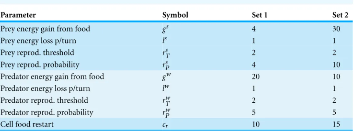
Table 4 Dynamics-related parameter sets.
Parameter Symbol Set 1 Set 2
Prey energy gain from food gs 4 30
Prey energy loss p/turn ls 1 1
Prey reprod. threshold rTs 2 2
Prey reprod. probability rPs 4 10
Predator energy gain from food gw 20 10
Predator energy loss p/turn lw 1 1
Predator reprod. threshold rTw 2 2
Predator reprod. probability rPw 5 5
Cell food restart cr 10 15
of parameters can be experimented with this model, these two sets are the basis for testing and comparing PPHPC implementations. We will refer to a combination of model size and parameter set as “size@set,” e.g., 400@1 for model size 400, parameter set 1.
While simulations of the PPHPC model are essentially non-terminating,1the number 1A non-terminating simulation is one for
which there is no natural event to specify the length of a run (Law, 2015).
of iterations,m, is set to 4,000, as it allows to analyze steady-state behavior for all the parameter combinations discussed here.
A NetLogo implementation
NetLogo is a well-documented programming language and modeling environment for ABMs, focused on both research and education. It is written in Scala and Java and runs on the Java Virtual Machine (JVM). It uses a hybrid interpreter and compiler that partially compiles ABM code to JVM bytecode (Sondahl, Tisue & Wilensky, 2006). It comes with powerful built-in procedures and is relatively easy to learn, making ABMs more accessible to researchers without programming experience (Martin et al., 2012). Advantages of having a NetLogo version include real-time visualization of simulation, pseudo-code like model descriptions, simplicity in changing and testing different model
aspects and parameters, and command-line access for batch runs and cycling through different parameter sets, even allowing for multithreaded simultaneous execution of
multiple runs. A NetLogo reference implementation is also particularly important as a point of comparison with other ABM platforms (Isaac, 2011).
The NetLogo implementation of PPHPC,Fig. 1, is based on NetLogo’s ownWolf Sheep Predationmodel (Wilensky, 1997), considerably modified to follow the ODD discussed in the previous section. Most NetLogo models will have at least asetupprocedure, to set up the initial state of the simulation, and agoprocedure to make the model run continuously (Wilensky, 2014). TheInit()andGetStats()processes (lines 1 and 2 of algorithm 1) are defined in thesetupprocedure, while the main simulation loop is implemented in thego
procedure. The latter has an almost one-to-one relation with its pseudo-code counterpart in Algorithm 1. By default, NetLogo shuffles agents before issuing them orders, which fits
Figure 1 NetLogo implementation of the PPHPC model.
Selection of focal measures
In order to analyze the output of a simulation model from a statistical point-of-view, we should first select a set of focal measures (FMs) which summarize each output.Wilensky & Rand (2007)use this approach in the context of statistical comparison of replicated models. Typically, FMs consist of long-term or steady-state means. However, being limited to analyze average system behavior can lead to incorrect conclusions (Law, 2015). Consequently, other measures such as proportions or extreme values can be used to assess model behavior. In any case, the selection of FMs is an empirical exercise and is always dependent of the model under study. A few initial runs are usually required in order to perform this selection.
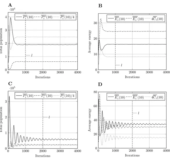
Figure 2 Typical model output for model size 400.Other model sizes have outputs which are similar, apart from a vertical scaling factor.Pirefers to total population,Eito mean energy andCito mean value of the countdown state variable,C. Superscriptsrelates to prey,wto predators, andcto cell-bound food.
Pci andCiare scaled for presentation purposes. (A) Population, param. set 1. (B) Energy, param. set 1. (C) Population, param. set 2. (D) Energy, param. set 2.
Table 5 Statistical summaries for each outputX.Xiis the value ofXat iterationi,mdenotes the last iteration, andlcorresponds to the iteration separating the transient and steady-state stages.
Statistic Description
max0≤i≤mXi Maximum value.
arg max0≤i≤mXi Iteration where maximum value occurs.
min0≤i≤mXi Minimum value.
arg min0≤i≤mXi Iteration where minimum value occurs.
Xss=m
i=l+1Xi/(m−l) Steady-state mean.
Sss=
m
i=l+1(Xi−Xss)2
Table 6 Values of a generic simulation output (under ‘Iterations’) fornreplications ofmiterations each (plus iteration 0, i.e. the initial state), and the respective FMs (under ‘Focal measures’).Values along columns are IID.
Rep. Iterations Focal measures
1 X10 X11 ... X1,m−1 X1,m maxX1 arg maxX1 minX1 arg minX1 Xss1 Sss1
2 X20 X21 ... X2,m−1 X2,m maxX2 arg maxX2 minX2 arg minX2 Xss2 Sss2
. .
. ... ... ... ... ... ... ... ... ... ...
n Xn0 Xn1 ... Xn,m−1 Xn,m maxXn arg maxXn minXn arg minXn Xssn Sssn
Collecting and preparing data for statistical analysis
LetXj0,Xj1,Xj2,...,Xjmbe an output from thejthsimulation run (rows under ‘Iterations’
inTable 6). TheXji’s are random variables that will, in general, be neither independent
nor identically distributed (Law, 2015), and as such, are not adequate to be used directly in many formulas from classical statistics (which are discussed in the next section). On the other hand, letX1i,X2i,...,Xnibe the observations of an output at iterationiforn
runs (columns under ‘Iterations’ inTable 6), where each run begins with the same initial conditions but uses a different stream of random numbers as a source of stochasticity. The Xji’s will now be independent and identically distributed (IID) random variables, to which
classical statistical analysis can be applied. However, individual values of the outputXat some iterationiare not representative ofXas a whole. Thus, we use the selected FMs as representative summaries of an output, as shown inTable 6, under ‘Focal measures.’ Taken column-wise, the observations of the FMs are IID (because they are obtained from IID replications), constituting asampleprone to statistical analysis.
Regarding steady-state measures,XssandSss, care must be taken with initialization bias, which may cause substantial overestimation or underestimation of the long-term performance (Sanchez, 1999). Such problems can be avoided by discarding data obtained during the initial transient period, before the system reaches steady-state conditions. The simplest way of achieving this is to use a fixed truncation point,l, for all runs with the same initial conditions, selected such that: (a) it systematically occurs after the transient state; and, (b) it is associated with a round and clear value, which is easier to communicate (Sanchez, 1999).Law (2015)suggests the use of Welch’s procedure (Welch, 1981) in order to empirically determinel. LetX0,X1,X2,...,Xmbe the averaged process taken column-wise
fromTable 6(columns under ‘Iterations’), such thatXi=nj=1Xji/nfori=0,1,...,m. The
averaged process has the same transient mean curve as the original process, but its variance is reduced by a factor ofn. A low-pass filter can be used to remove short-term fluctuations, leaving the long-term trend of interest, allowing us to visually determine a value oflfor which the averaged process seems to have converged. A moving average approach can be used for filtering:
Xi(w)=
w
s=−wXi+s
2w+1 ifi=w+1,...,m−w
i−1
s=−(i−1)Xi+s
2i−1 ifi=1,...,w
wherew, thewindow, is a positive integer such thatw6⌊m/4⌋. This value should be large enough such that the plot ofXi(w)is moderately smooth, but not any larger. A more
in-depth discussion of this procedure is available inWelch (1981)andLaw (2015).
Statistical analysis of focal measures
LetY1,Y2,...,Ynbe IID observations of some FM with finite population meanµand
finite population varianceσ2(i.e. any column under ‘Focal measures’ inTable 6). Then, as described byLaw (2007)andLaw (2015), unbiased point estimators forµandσ2are given by
Y(n)=
n
j=1Yj
n (6)
and
S2(n)=
n
j=1[Yj−Y(n)]2
n−1 (7)
respectively.
Another common statistic usually determined for a given FM is the confidence interval (CI) forY(n), which can be defined in several different ways. Thet-distribution CI is
commonly used for this purpose (Law, 2007;Law, 2015), although it has best coverage for normally distributed samples, which is often not the case for simulation models in general (Sargent, 1976;Law, 2015) and agent-based models in particular (Helbing & Balietti, 2012). If samples are drawn from populations with multimodal, discrete or strongly skewed distributions, the usefulness oft-distribution CIs is further reduced. While there is not much to do in the case of multimodal distributions,Law (2015)proposes the use of the CI developed byWillink (2005), which takes distribution skewness into account. Furthermore, CIs for discrete distributions are less studied and usually assume data follows a binomial distribution, presenting some issues of its own (Brown, Cai & DasGupta, 2001). As suggested byRadax & Rengs (2010), we focus on providing a detailed assessment of the distributional properties of the different FMs, namely whether they are sufficiently
“normal” such that normality-assuming (parametric) statistical techniques can be applied, not only for CI estimation, but also for model comparison purposes.
The normality of a data set can be assessed graphically or numerically (Park, 2008). The former approach is intuitive, lending itself to empirical interpretation by providing a way to visualize how random variables are distributed. The latter approach is a more objective and quantitative form of assessing normality, providing summary statistics and/or statistics tests of normality. In both approaches, specific methods can be either descriptive or theory-driven, as shown inTable 7.
For this study we chose one method of each type, as shown in boldface inTable 7. This approach not only provides a broad overview of the distribution under study, but is also important because no single method can provide a complete picture of the distribution.
Table 7 Methods for assessing the normality of a data set, adapted fromPark (2008).Boldface methods are used in this study.
Graphical methods Numerical methods
Descriptive Histogram, Box plot, Dot plot Skewness, Kurtosis
Theory-driven Q–Q plot, P-P plot Shapiro-Wilk, Anderson-Darling, Cramer-von Mises, Kolmogorov-Smirnov, Jarque-Bera and other tests
intervals (bins), and counting how many values fall in each interval. AQ–Q plotcompares the distribution of a data set with a specific theoretical distribution (e.g., the normal distribution) by plotting their quantiles against each other (thus “Q–Q”). If the two distributions match, the points on the plot will approximately lie on they=xline. While a histogram gives an approximate idea of the overall distribution, the Q–Q plot is more adequate to see how well a theoretical distribution fits the data set.
Concerning numerical methods,Skewnessmeasures the degree of symmetry of a probability distribution about its mean, and is a commonly used metric in the analysis of simulation output data (Sargent, 1976;Nakayama, 2008;Law, 2015). If skewness is positive, the distribution is skewed to the right, and if negative, the distribution is skewed to the left. Symmetric distributions have zero skewness, however, the converse is not necessarily true, e.g., skewness will also be zero if both tails of an asymmetric distribution account for half the total area underneath the probability density function. In the case of theory-driven nu-merical approaches, we select theShapiro-Wilk(SW) test (Shapiro & Wilk, 1965), as it has been shown to be more effective when compared to several other normality tests (Razali &
Wah, 2011). We focus on thep-value of this test (instead of the test’s ownWstatistic), as it is an easily interpretable measure. The null-hypothesis of this test is that the data set, or sample, was obtained from a normally distributed population. If thep-value is greater than a predetermined significance levelα, usually 0.01 or 0.05, then the null hypothesis cannot be rejected. Conversely, ap-value less thanαimplies the rejection of the null hypothesis, i.e., that the sample was not obtained from a normally distributed population.
RESULTS
A total of 30 replications,r=1,...,30, were performed with NetLogo 5.1.0 for each combination of model sizes (Table 3) and parameters sets (Table 4). Each replicationrwas performed with a PRNG seed obtained by taking the MD5 checksum ofrand converting the resulting hexadecimal string to a 32-bit integer (the maximum precision accepted by NetLogo), guaranteeing some independence between seeds, and consequently, between replications. The list of seeds is provided inTable S1.
Determining the steady-state truncation point
Figure 3 Moving average of outputs for model size 400 withw=10.Other model sizes produce similar results, apart from a vertical scaling factor. The dashed vertical line corresponds to iterationlafter which the output is considered to be in steady-state. (A) Population moving average, param. set 1. (B) Energy moving average, param. set 1. (C) Population moving average, param. set 2. (D) Energy moving average, param. set 2.
‘Methodology’, we select the steady-state truncation point to bel=1,000 for parameter set 1, andl=2,000 for parameter set 2. These are round values which appear to occur after the transient stage. Other model sizes produce similar results, apart from a vertical scaling factor, which means that these values oflare also applicable in those cases.
Analyzing the distributions of focal measures
The six statistic summaries for each FM, namely mean, sample variance,p-value of the SW test, skewness, histogram and Q–Q plot, are shown inTables S2.1–S2.10for all model size and parameter set combinations. The number of bins in the histograms is set to the minimum between 10 (an appropriate value for a sample size of 30) and the number of unique values in the data set.
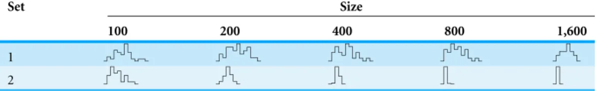
Table 8 Histograms for the several size@set combinations of the arg maxPsiFM.
Set Size
100 200 400 800 1,600
1 2
However, FMs taken fromarg maxandarg minoperators only yield integer (discrete) values, which correspond to specific iterations. The same is true formaxandminof population outputs, namelyPsi,Piw, andPci. This can be problematic for statistic summaries taken from integer-valued FMs with a small number of unique values. For example, the SW test will not be very informative in such cases, and cannot even be performed if all observations yield the same value (e.g.,arg maxofPci for 800@1,Table S2.4). Nonetheless, distributional properties of a FM can dramatically change for different model size and
parameter set combinations. For example, for parameter set 2, observations of thearg maxofPci span many different values for model size 200 (Table S2.7), while for size 1,600
(Table S2.10) they are limited to only three different values. Summary statistics appropriate
for continuous distributions could be used in the former case, but do not provide overly useful information in the latter. In order to maintain a consistent approach, our discussion will continue mainly from a continuous distribution perspective, more specifically by analyzing how closely a given FM follows the normal distribution, though we superficially examine its discrete nature when relevant.
Distribution of focal measures over the several size@set combinations In the next paragraphs we describe the distributional behavior of each FM, and when useful, repeat in a compact fashion some of the information provided inTables S2.1–S2.10.
maxPsi. The SWp-value is consistently above the 5% significance level, skewness is usually low and with an undefined trend, and the Q–Q plots mostly follow they=xline. Although there are borderline cases, such as 800@1 and 1,600@2, the summary statistics show that the maximum prey population FM generally follows an approximately normal distribution.
arg maxPsi. This FM follows an approximately normal distribution for smaller sizes of parameter set 1, but as model size grows larger, the discrete nature of the data clearly stands out. This behavior is more pronounced for parameter set 2 (which yields simulations inherently larger than parameter set 1), such that, for 1,600@2, all observations yield the same value (i.e., 70).Table 8shows, using histograms, how the distribution qualitatively evolves over the several size@set combinations.
minPsi. Two very different behaviors are observed for the two parameter sets. In the
case of parameter set 1, this FM has a slightly negatively skewed distribution, with some
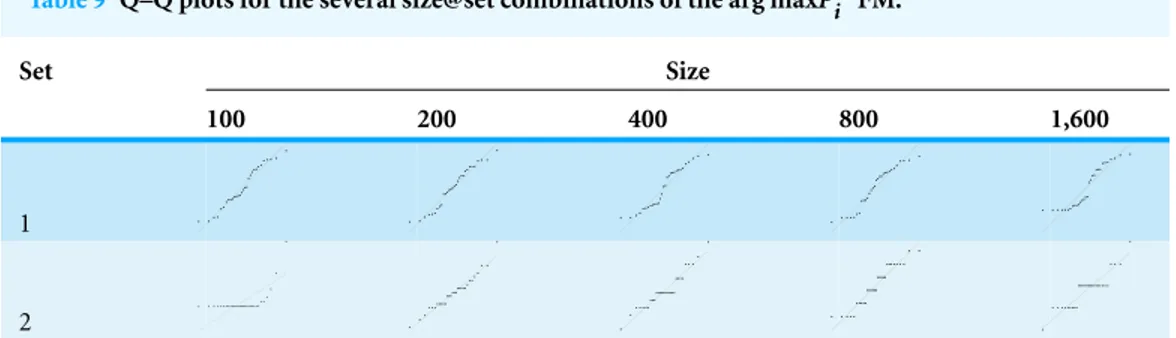
Table 9 Q–Q plots for the several size@set combinations of the arg maxPwi FM.
Set Size
100 200 400 800 1,600
1
2
(this is quite visible in some histograms). However, for parameter set 2, the data is more concentrated on a single value, more so for larger sizes. Note that this single value is the initial number of prey, which means that, in most cases, the minimum number of prey never drops below its initial value.
arg minPsi. This FM follows a similar pattern to the previous one, but more pronounced in terms of discreteness, namely for parameter set 1. For parameter set 2, sizes 100 and 200, the distribution is bimodal, with the minimum prey population occurring at iteration zero (i.e. initial state) or around iteration 200, while for larger sizes, the minimum always occurs at iteration zero.
Pisss. The prey population steady-state mean seems to generally follow a normal distribution, the only exception being 400@2, in which some departure from normality is observed, as denoted by a SWp-value below 0.05 and a few outliers in the Q–Q plot.
Sss(Psi). For most size@set combinations this FM does not present large departures from normality. However, skewness is always positive.
maxPwi . This FM presents distributions which are either considerably skewed or relatively normal. The former tend to occur for smaller model sizes, while the latter for larger sizes, although this trend is not totally clear. The 800@2 sample is a notable case, as it closely follows a normal distribution, with a symmetric histogram, approximately linear Q–Q plot, and a SWp-value of 0.987.
arg maxPwi . Interestingly, for parameter set 1, this FM seems to follow a uniform distribution. This is more or less visible in the histograms, but also in the Q–Q plots, because when we plot uniform data points against a theoretical normal distribution in a Q–Q plot we get the “stretched-S” pattern which is visible in this case (Table 9). For parameter set 2, the distribution seems to be more normal, or even binomial as the discreteness of the data starts to stand-out for larger model sizes; the only exception is for size 100, which presents a multimodal distribution.
arg minPwi . This FM displays an approximately normal distribution. However, for larger simulations (i.e. mainly for parameter set 2) the discrete nature of the data becomes more apparent.
Piwss. The steady-state mean of predator population apparently follows a normal distribution. This is confirmed by all summary statistics, such as the SWp-value, which is above 0.05 for all size@set combinations.
Sss(Pwi ). Departure from normality is not large in most cases (200@2 and 800@2 are exceptions, although the former due to a single outlier), but the trend of positive skewness is again observed for this statistic.
maxPci. The maximum available cell-bound food seems to have a normal distribution, although 400@2 has a few outliers which affect the result of the SWp-value (which,
nonetheless, is above 0.05).
arg maxPci. The behavior of this FM is again quite different between parameter sets. For
the first parameter set, the discrete nature of the underlying distribution stands out, with no more than three unique values for size 100, down to a single value for larger sizes, always centered around the value 12 (i.e. the maximum available cell-bound food tends to occur at iteration 12). For the second parameter set, distribution is almost normal for sizes above 200, centered around iteration 218, although its discreteness shows for larger sizes, namely for size 1,600, which only presents three distinct values. For size 100, most values fall in iteration 346, although two outliers push the mean up to 369.5.
minPci. This FM displays an apparently normal distribution for all model sizes and parameter sets, with the exception of 800@1, which has a few outliers at both tails of the distribution, bringing down the SWp-value barely above the 5% significance level.
arg minPci. In this case, the trend is similar for both parameter sets, i.e. the distribution seems almost normal, but for larger sizes the underlying discreteness becomes apparent. This is quite clear for parameter set 2, as shown inTable 10, where the SW testp-value decreases as the discreteness becomes more visible in the histograms and Q–Q plots.
Picss. For this FM there is not a significant departure from normality. The only exception is for 800@1, but only due to a single outlier.
Sss(Pci). Like in previous cases, the steady-state sample standard deviation does not stray too far from normality, but consistently shows a positive skewness.
maxEsi. For sizes 100 and 200 of both parameter sets, the maximum of the mean prey energy presents a positively skewed, lognormal-like distribution. For larger sizes, distributions tend to be more normal-like. This trend is clear when analyzing how the
Table 10 Three statistical summaries for the several sizes of the arg minPci FM for parameter set 2.Row ‘SW’ contains the SW testp-values, while the corresponding histograms and Q–Q plots are in rows ‘Hist.’ and ‘Q–Q’, respectively.
Set Size
100 200 400 800 1,600
SW 0.437 0.071 0.062 0.011 <0.001
Hist.
Q–Q
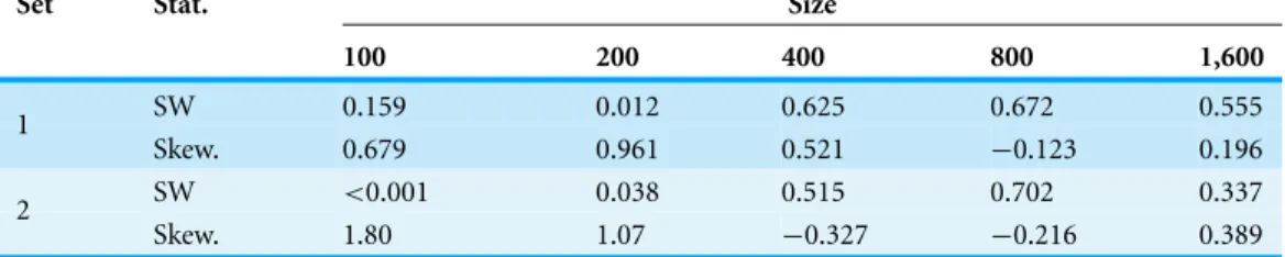
Table 11 p-values for the SW test (row ‘SW’) and skewness (row ‘Skew.’) for the several size@set combinations of the maxEsiFM.
Set Stat. Size
100 200 400 800 1,600
SW 0.159 0.012 0.625 0.672 0.555
1
Skew. 0.679 0.961 0.521 −0.123 0.196
SW <0.001 0.038 0.515 0.702 0.337
2
Skew. 1.80 1.07 −0.327 −0.216 0.389
arg maxEsi. For parameter set 1, the distribution is approximately normal for smaller sizes, with the underlying discreteness becoming apparent for larger sizes, centering around iteration 49. For parameter set 2, the data set revolves around a limited set of unique values (centered at iteration 16), following a poisson-like distribution, except for size 100, which displays a bimodal behavior.
minEsi. This FM seems to follow an approximately normal distribution.
arg minEsi. In the case of parameter set 1, this FM has distributions with a single value: zero. This means that the minimum mean prey energy occurs at the initial state of the simulation. From there onwards, mean prey energy is always higher. The situation is notably different for the second parameter set, where minimum mean prey energy can
occur at several different iterations centered around iteration 88. Distribution seems to be
binomial or Poisson-like.
Esiss. Although the histograms are not very clear, the Q–Q plots and thep-values from the SW test suggest that this FM follows a normal distribution.
Sss(Esi). This FM does not seem to stray much from normality, except in the case of 1,600@1 and 200@2, which are affected by outliers. The tendency for the steady-state
maxEwi . The maximum of mean predator energy follows an approximately normal distribution, though for 100@1 there are a few replications which produce unexpected results.
arg maxEwi . In most cases, this FM approximately follows a normal distribution. There are several exceptions though. For the second parameter set and sizes above 400, the FM starts to display its discrete behavior, following a Poisson-like distribution. Less critically, an outlier “ruins” normality for 100@1.
minEwi . Apart from a few outliers with some parameter combinations, this FM generally seems to follow a normal distribution.
arg minEwi . Perhaps with the exception of 100@1 and 200@1, the iteration where the minimum of mean predator energy occurs seems best described with a discrete, Poisson-like distribution.
Ewi ss. This FM generally follows a normal distribution. However, 1,600@1 shows a salient second peak (to the right of the histogram, also visible in the Q–Q plot), affecting the
resulting SWp-value, which is below the 1% significance threshold.
Sss(Ewi ). This FM follows a positively skewed unimodal distribution, in the same line as the steady-state sample standard deviation of other outputs. Note the outlier in 200@2, also observed for theSss(Pwi )FM, which is to be excepted as both FMs are related to predator dynamics.
maxCi. The samples representing the maximum of the meanCstate variable are most
likely drawn from a normal distribution. Most histograms are fairly symmetric (which is corroborated by the low skewness values), the Q–Q plots are generally linear, and the SW
p-value never drops below 0.05 significance.
arg maxCi. For smaller model sizes this FM follows a mostly normal distribution, but as
with other iteration-based FMs, the underlying discreteness of the distribution starts to show at larger model sizes, especially for the second parameter set.
minCi. For most size@set combinations, the minimum of the meanCstate variable
seems to be normally distributed. Nonetheless, a number of observations for 400@2 yield unexpected values, making the respective distribution bimodal and distorting its normality (though the respective SWp-value does not drop below 0.05).
arg minCi. As in some previous cases, this FM displays different behavior depending
on the parameter set. For the first parameter set, practically all observations have the same value, 10, which means the minimum of the meanCstate variable is obtained at iteration 10. Only model sizes 100 and 200 have some observations representing iterations 11 and/or 12. Parameter set 2 yields a different dynamic, with an average iteration of 216
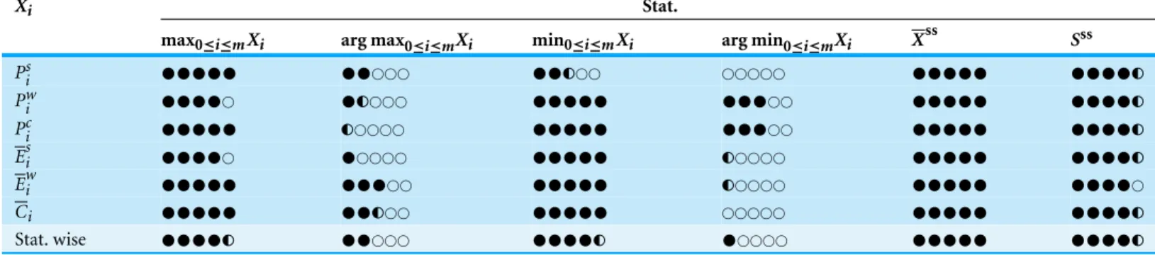
Table 12 Empirical classification (from 0 to 5) of each FM according to how close it follows the normal distribution for the tested size@set combinations.The last row outlines the overall normality of each statistic.
Xi Stat.
max0≤i≤mXi arg max0≤i≤mXi min0≤i≤mXi arg min0≤i≤mXi Xss Sss
Pis
•••••
••
⃝⃝⃝••
◐⃝⃝ ⃝⃝⃝⃝⃝•••••
••••
◐Piw
••••
⃝•
◐⃝⃝⃝•••••
•••
⃝⃝•••••
••••
◐Pic
•••••
◐⃝⃝⃝⃝•••••
•••
⃝⃝•••••
••••
◐Esi
••••
⃝•
⃝⃝⃝⃝•••••
◐⃝⃝⃝⃝•••••
••••
◐Ewi
•••••
•••
⃝⃝•••••
◐⃝⃝⃝⃝•••••
••••
⃝Ci
•••••
••
◐⃝⃝•••••
⃝⃝⃝⃝⃝•••••
••••
◐Stat. wise
••••
◐••
⃝⃝⃝••••
◐•
⃝⃝⃝⃝•••••
••••
◐distant outliers). While sizes 200 and 400 follow an approximately normal distribution, larger sizes seem more fit to be analyzed using discrete distributions such as Poisson or binomial.
Ci ss
. This FM follows an approximately normal distribution. While most size/parameter combinations have a few outliers, only for 800@1 is the existing outlier capable of making the SW test produce ap-value below the 5% significance threshold.
Sss(Ci). Although passing the SW normality test (p-value>0.05) in most cases, we
again note the positive skewness of the steady-state sample standard deviation samples, suggesting that distributions such as Weibull or Lognormal maybe a better fit.
Statistics-wise distribution trends
Table 12summarizes the descriptions given in the previous section. It was built by assigning an empirical classification from 0 to 5 to each FM according to how close it follows the normal distribution for the tested size@set combinations. More specifically, individual classifications were determined by analyzing the information provided in Tables S2.1–S2.10, prioritizing the SW test result (i.e. if thep-value is above 0.01 and/or 0.05) and distributional discreteness (observable in the Q–Q plots). This classification can be used as a guide to whether parametric or non-parametric statistical methods should be used to further analyze the FMs or to compare FMs of different PPHPC implementations.
The last row shows the average classification of individual outputs for a given statistic, outlining its overall normality.
Themaxandminstatistics yield mostly normal distributions, although care should be taken when the maximum or minimum systematically converge to the same value, e.g., when they occur at iteration zero. Nonetheless, parametric methods seem adequate for FMs drawn from these statistics. The same does not apply to thearg maxandarg min
FMs. Consequently, parametric methods will most likely be suitable for this statistic. Finally, FMs based on the steady-state sample standard deviation display normal-like behavior, albeit with consistently positive skewness; in fact, they are probably better represented by a Weibull or Lognormal distribution. While parametric methods may be used for this statistic, results should be interpreted cautiously.
DISCUSSION
In this paper, the PPHPC model is completely specified, and an exhaustive analysis of the respective simulation outputs is performed. Regarding the latter, after determining the mean and variance of the several FMs, we opted to study their distributional properties instead of proceeding with the classical analysis suggested by simulation output analysis literature (i.e., the establishment of CIs.). This approach has a number of practical uses. For example, if we were to estimate CIs for FMs drawn from the steady-state mean, we could uset-distribution CIs with some confidence, as these FMs display an approximately normal distribution. If we did the same for FMs drawn from the steady-state sample standard deviation, theWillink (2005)CI would be preferable, as it accounts for the skewness displayed by these FMs. Estimating CIs without a good understanding of the underlying distribution can be misleading, especially if the distribution is multimodal. The approach taken here is also useful for comparing different PPHPC implementations.
If we were to comparemaxormin-based FMs, which seem to follow approximately normal distributions, parametric tests such as thet-test would most likely produce valid conclusions. On the other hand, if we comparearg maxorarg min-based FMs, non-parametric tests, such as the Mann-WhitneyUtest (Gibbons & Chakraborti, 2011), would be more adequate, as these FMs do not usually follow a normal distribution.
However, the scope of the PPHPC model is significantly broader. For example, in Fachada et al. (2015b), PPHPC is reimplemented in Java with several user-selectable parallelization strategies. The goal is to clarify which are the best parallelization approaches for SABMs in general. An-sample statistical test is applied to each FM, for all implemen-tations and strategies simultaneously, in order to verify that these do not yield dissimilar results. InFachada et al. (2015a), PPHPC is used for presenting a novel model-independent comparison technique which directly uses simulation outputs, bypassing the need of selecting model-specific FMs.
The PPHPC model is made available to other researchers via the source code, in addition to the specification presented here. All the data analyzed in this paper is also available asSupplemental Information. PPHPC can be used as a pure computational model without worrying with aspects like visualization and user interfaces, allowing for direct performance comparison of different implementations.
CONCLUSION
many ABMs have been published, proper model description and analysis is lacking in the scientific literature, and thus this paper can be seen as a guideline or methodology to improve model specification and communication in the field. Furthermore, PPHPC aims to be a standard model for research in agent-based modeling and simulation, such as, but not limited to, statistical model comparison techniques, performance comparison of parallel implementations, and testing the influence of different PRNGs on the statistical
accuracy of simulation output.
ADDITIONAL INFORMATION AND DECLARATIONS
Funding
This work was supported by the Fundac¸˜ao para a Ciˆencia e a Tecnologia (FCT) projects UID/EEA/50009/2013, UID/MAT/04561/2013 and (P. RD0389) Incen-tivo/EEI/LA0009/2014, and partially funded with grant SFRH/BD/48310/2008, also from FCT. The author Vitor V. Lopes acknowledges the financial support from the Prometeo project of SENESCYT (Ecuador). The funders had no role in study design, data collection and analysis, decision to publish, or preparation of the manuscript.
Grant Disclosures
The following grant information was disclosed by the authors:
Fundac¸˜ao para a Ciˆencia e a Tecnologia (FCT): UID/EEA/50009/2013, UID/MAT/04561/2013, Incentivo/EEI/LA0009/2014, SFRH/BD/48310/2008. SENESCYT: Prometeo project.
Competing Interests
The authors declare there are no competing interests.
Author Contributions
• Nuno Fachada conceived and designed the experiments, performed the experiments, analyzed the data, wrote the paper, prepared figures and/or tables, performed the computation work, reviewed drafts of the paper.
• Vitor V. Lopes conceived and designed the experiments, wrote the paper, reviewed drafts of the paper.
• Rui C. Martins analyzed the data, reviewed drafts of the paper.
• Agostinho C. Rosa contributed reagents/materials/analysis tools, reviewed drafts of the paper.
Data Availability
The following information was supplied regarding data availability: https://github.com/fakenmc/pphpc/tree/netlogo.
Supplemental Information
REFERENCES
Axtell R, Axelrod R, Epstein JM, Cohen MD. 1996. Aligning simulation models: a case study and results.Computational and Mathematical Organization Theory 1(2):123–141 DOI 10.1007/BF01299065.
Bigbee A, Cioffi-Revilla C, Luke S. 2007.Replication of sugarscape using MASON. In: Terano T, Kita H, Deguchi H, Kijima K, eds.Agent-based approaches in economic and social complex systems IV,Springer series on agent based social systems,vol. 3. Tokyo: Springer, 183–190. Brown LD, Cai TT, DasGupta A. 2001.Interval estimation for a binomial proportion.Statistical
Science16(2):101–117.
D’Souza R, Lysenko M, Rahmani K. 2007.Sugarscape on steroids: simulating over a million agents at interactive rates. In:Proceedings of agent 2007 conference, Chicago, USA.Available athttp:// www.me.mtu.edu/∼rmdsouza/Papers/2007/SugarScape GPU.pdf.
Edmonds B, Hales D. 2003.Replication, replication and replication: some hard lessons from model alignment.Journal of Artificial Societies and Social Simulation6(4):11.
Epstein J, Axtell R. 1996.Growing artificial societies: social science from the bottom up. Cambridge: MIT Press.
Fachada N. 2008.Agent-based simulation of the immune system. Master’s thesis, Instituto Superior T´ecnico, Universidade T´ecnica de Lisboa, Lisboa.
Fachada N, Lopes VV, Martins RC, Rosa AC. 2015a. Model-independent comparison of simulation output. ArXiv preprint.arXiv:1509.09174.
Fachada N, Lopes VV, Martins RC, Rosa AC. 2015b.Parallelization strategies for spatial agent-based models. ArXiv preprint.arXiv:1507.04047.
Gibbons JD, Chakraborti S. 2011.Nonparametric statistical inference. New York: Springer. Ginovart M. 2014.Discovering the power of individual-based modelling in teaching and learning:
The study of a predator-prey system.Journal of Science Education and Technology23(4):496–513 DOI 10.1007/s10956-013-9480-6.
Goldsby ME, Pancerella CM. 2013.Multithreaded agent-based simulation. In:Proceedings of the 2013 winter simulation conference: simulation: making decisions in a complex world, WSC’13. Washington, D.C.: IEEE Press, 1581–1591.
Grimm V, Berger U, DeAngelis D, Polhill J, Giske J, Railsback S. 2010. The ODD protocol: a review and first update. Ecological Modelling 221(23):2760–2768 DOI 10.1016/j.ecolmodel.2010.08.019.
Helbing D, Balietti S. 2012.How to do agent-based simulations in the future: from modeling social mechanisms to emergent phenomena and interactive systems design. In: Social self-organization,Agent-based modeling.New York: Springer, 25–70.
Hiebeler D. 1994.The Swarm simulation system and individual-based modeling. SFI Working Paper: 1994-11-065.
Isaac AG. 2011.The ABM template models: A reformulation with reference implementations. Journal of Artificial Societies and Social Simulation14(2):5DOI 10.18564/jasss.1749.
Kahn K. 2007.Comparing multi-agent models composed from micro-behaviours. In: Rouchier J, Cioffi-Revilla C, Polhill G, Takadama K, eds.M2M 2007: third international model-to-model workshop, Marseilles, France.
Kelton WD. 1997.Statistical analysis of simulation output. In:Proceedings of the 29th conference on winter simulation, WSC’97. Piscataway: IEEE Computer Society, 23–30.
Law AM. 2007.Statistical analysis of simulation output data: the practical state of the art. In:Simulation conference, 2007 winter. Piscataway: IEEE, 77–83.
Law AM. 2015.Simulation modeling and analysis. 5th edition. New York: McGraw-Hill. Lotka A. 1925.Elements of physical biology. Philadelphia: Lippincott Williams and Wilkins. Lysenko M, D’Souza R. 2008.A framework for megascale agent based model simulations on
graphics processing units.Journal of Artificial Societies and Social Simulation11(4):10. Lytinen SL, Railsback SF. 2012.The evolution of agent-based simulation platforms: a review of
NetLogo 5.0 and ReLogo. In:Proceedings of the fourth international symposium on agent-based modeling and simulation, Vienna, Austria.Available athttp://www2.econ.iastate.edu/tesfatsi/ NetLogoReLogoReview.LytinenRailsback2012.pdf.
Macal CM, North MJ. 2008.Agent-based modeling and simulation: ABMS examples. In:Proceedings of the 40th conference on winter simulation, WSC’08. Williston: Winter Simulation Conference Foundation, 101–112.
Macal C, North M. 2010.Tutorial on agent-based modelling and simulation.Journal of Simulation 4(3):151–162DOI 10.1057/jos.2010.3.
Martin BT, Zimmer EI, Grimm V, Jager T. 2012.Dynamic energy budget theory meets individual-based modelling: a generic and accessible implementation.Methods in Ecology and Evolution3(2):445–449DOI 10.1111/j.2041-210X.2011.00168.x.
Merlone U, Sonnessa M, Terna P. 2008.Horizontal and vertical multiple implementations in a model of industrial districts.Journal of Artificial Societies and Social Simulation11(2):5. M¨uller B, Balbi S, Buchmann CM, de Sousa L, Dressler G, Groeneveld J, Klassert CJ, Le QB,
Millington JDA, Nolzen H, Parker DC, Polhill JG, Schl¨uter M, Schulze J, Schwarz N, Sun Z, Taillandier P, Weise H. 2014.Standardised and transparent model descriptions for agent-based models: Current status and prospects.Environmental Modelling & Software55:156–163 DOI 10.1016/j.envsoft.2014.01.029.
Nakayama MK. 2008.Statistical analysis of simulation output. In:Proceedings of the 40th conference on winter simulation, WSC’08. Williston: Winter Simulation Conference Foundation, 62–72.
Ottino-Loffler J, Rand W, Wilensky U. 2007.Co-evolution of predators and prey in a spatial model. In:GECCO 2007. New York: SIGEVO.
Park HM. 2008.Univariate analysis and normality test using SAS, Stata, and SPSS. Working Paper. The University Information Technology Services (UITS) Center for Statistical and Mathematical Computing, Indiana University.Available athttp://education.exeter.ac.uk/download.php? id=10414.
Radax W, Rengs B. 2010.Prospects and pitfalls of statistical testing: Insights from replicating the demographic prisoner’s dilemma.Journal of Artificial Societies and Social Simulation 13(4):1DOI 10.18564/jasss.1634.
Railsback S, Lytinen S, Grimm V. 2005.StupidModel and extensions: a template and teaching tool for agent-based modeling platforms. Seattle: Swarm Development Group.
Railsback S, Lytinen S, Jackson S. 2006. Agent-based simulation platforms: review and development recommendations.Simulation82(9):609–623DOI 10.1177/0037549706073695. Razali NM, Wah YB. 2011.Power comparisons of Shapiro-Wilk, Kolmogorov-Smirnov, Lilliefors
and Anderson-Darling tests.Journal of Statistical Modeling and Analytics2(1):21–33.
Reynolds CW. 1987.Flocks, herds and schools: a distributed behavioral model.ACM SIGGRAPH Computer Graphics21(4):25–34DOI 10.1145/37402.37406.
Rollins ND, Barton CM, Bergin S, Janssen MA, Lee A. 2014.A computational model library for publishing model documentation and code.Environmental Modelling & Software61:59–64 DOI 10.1016/j.envsoft.2014.06.022.
Sallach D, Mellarkod V. 2005.Interpretive agents: A heatbug reference simulation. In:Proceedings of agent 2005 conference on generative social processes, models, and mechanisms. 693–705. Sanchez SM. 1999.ABC’s of output analysis. In:Simulation conference proceedings, 1999 winter.
vol. 1. Piscataway: IEEE, 24–32.
Sargent RG. 1976.Statistical analysis of simulation output data.ACM SIGSIM Simulation Digest 7(4):39–50DOI 10.1145/1013610.807298.
Shapiro SS, Wilk MB. 1965.An analysis of variance test for normality (complete samples). Biometrika52(3/4):591–611DOI 10.1093/biomet/52.3-4.591.
Shook E, Wang S, Tang W. 2013.A communication-aware framework for parallel spatially explicit agent-based models. International Journal of Geographical Information Science 27(11):2160–2181DOI 10.1080/13658816.2013.771740.
Smith M. 1991.Using massively-parallel supercomputers to model stochastic spatial predator-prey systems.Ecological Modelling58(1):347–367DOI 10.1016/0304-3800(91)90045-3.
Sondahl F, Tisue S, Wilensky U. 2006.Breeding faster turtles: Progress towards a NetLogo compiler. In:Proceedings of the agent 2006 conference on social agents, Chicago, IL, USA. Available athttps://ccl.northwestern.edu/papers/sond tis wil breeding.pdf.
Standish RK. 2008. Going stupid with EcoLab. Simulation 84(12):611–618 DOI 10.1177/0037549708097146.
Tang W, Wang S. 2009.HPABM: a hierarchical parallel simulation framework for spatially-explicit agent-based models.Transactions in GIS13(3):315–333DOI 10.1111/j.1467-9671.2009.01161.x. Tatara E, North M, Howe T, Collier N, Vos J. 2006.An introduction to Repast modeling using
a simple predator-prey example. In: Sallach DL, Macal CM, North MJ, eds.Proceedings of the agent 2006 conference on social agents: results and prospects, vol. ANL/DIS-06-7. Chicago: Argonne National Laboratory and The University of Chicago, 83–94.
Volterra V. 1926.Fluctuations in the abundance of a species considered mathematically.Nature 118:558–560DOI 10.1038/118558a0.
Welch PD. 1981. On the problem of the initial transient in steady-state simulation. Yorktown Heights: IBM Watson Research Center.
Wilensky U. 1997.NetLogo wolf sheep predation model.Available athttp://ccl.northwestern.edu/ netlogo/models/WolfSheepPredation.
Wilensky U. 1999.NetLogo.Available athttps://ccl.northwestern.edu/netlogo/.
Wilensky U. 2004.NetLogo heatbugs model.Available athttp://ccl.northwestern.edu/netlogo/ models/Heatbugs.
Wilensky U. 2014.NetLogo 5.1.0 user manual. Evanston: Northwestern University.Available at http://ccl.northwestern.edu/netlogo/docs/.
Wilensky U, Rand W. 2007.Making models match: replicating an agent-based model.Journal of Artificial Societies and Social Simulation10(4):2.