NPGD
1, 1919–1946, 2014Features of fluid flows in strongly nonlinear internal
solitary waves
S. Semin et al.
Title Page
Abstract Introduction
Conclusions References
Tables Figures
◭ ◮
◭ ◮
Back Close
Full Screen / Esc
Printer-friendly Version
Interactive Discussion
Discussion
P
a
per
|
Discussion
P
a
per
|
Discussion
P
a
per
|
Discussion
P
a
per
Nonlin. Processes Geophys. Discuss., 1, 1919–1946, 2014 www.nonlin-processes-geophys-discuss.net/1/1919/2014/ doi:10.5194/npgd-1-1919-2014
© Author(s) 2014. CC Attribution 3.0 License.
This discussion paper is/has been under review for the journal Nonlinear Processes in Geophysics (NPG). Please refer to the corresponding final paper in NPG if available.
Features of fluid flows in strongly
nonlinear internal solitary waves
S. Semin1, O. Kurkina1, A. Kurkin1, T. Talipova1,2, E. Pelinovsky1,2,3, and E. Churaev1
1
Nizhny Novgorod State Technical University n.a. R. Alekseev, Nizhny Novgorod, Russia 2
Institute of Applied Physics, Nizhny Novgorod, Russia 3
National Research University – Higher School of Economics, Moscow, Russia
Received: 30 November 2014 – Accepted: 2 December 2014 – Published: 18 December 2014
Correspondence to: A. Kurkin ([email protected])
NPGD
1, 1919–1946, 2014Features of fluid flows in strongly nonlinear internal
solitary waves
S. Semin et al.
Title Page
Abstract Introduction
Conclusions References
Tables Figures
◭ ◮
◭ ◮
Back Close
Full Screen / Esc
Printer-friendly Version
Interactive Discussion
Discussion
P
a
per
|
Discussion
P
a
per
|
Discussion
P
a
per
|
Discussion
P
a
per
|
Abstract
The characteristics of highly nonlinear solitary internal waves (solitons) are calculated within the fully nonlinear numerical model of the Massachusetts Institute of Technol-ogy. The verification and adaptation of the model is based on the data from laboratory experiments. The present paper also compares the results of our calculations with the
5
calculations performed in the framework of the fully nonlinear Bergen Ocean Model. The comparison of the computed soliton parameters with the predictions of the weakly nonlinear theory based on the Gardner equation is given. The occurrence of reverse flow in the bottom layer directly behind the soliton is confirmed in the numerical simula-tions. The trajectories of Lagrangian particles in the internal soliton on the surface, on
10
the pycnocline and near the bottom are computed.
1 Introduction
Solitons of internal waves are widely observed in the World Ocean (Ostrovsky and Stepanyants, 1989; Jackson, 2004; Vlasenko et al., 2005; Helfrich and Melville, 2006; Apel et al., 2007) and have been the object of study for a number of decades. Nonlinear
15
internal waves affect underwater biological community (Shapiro et al., 2000;
Donald-son et al., 2008), cause sediment transport (Bogucki and Redekopp, 1999; Stastna and Lamb, 2008), force the platforms and pipelines (Fraser, 1999; Cai et al., 2003, 2006; Song et al., 2011), affect the propagation of acoustic signals (Apel et al., 2007; Warn-Varnas, 2009; Chin-Bing, 2009). A lot of numerical models have been developed
20
to simulate solitary internal wave generation, propagation and transformation, and we cannot cite all the important papers now. Laboratory experiments allow studying the soliton characteristics in controlled conditions and validating the numerical models (Os-trovsky and Stepanyants, 2005; Carr and Davies, 2006; Carr et al., 2008; Cheng et al., 2008).
NPGD
1, 1919–1946, 2014Features of fluid flows in strongly nonlinear internal
solitary waves
S. Semin et al.
Title Page
Abstract Introduction
Conclusions References
Tables Figures
◭ ◮
◭ ◮
Back Close
Full Screen / Esc
Printer-friendly Version
Interactive Discussion
Discussion
P
a
per
|
Discussion
P
a
per
|
Discussion
P
a
per
|
Discussion
P
a
per
The simplest and most obvious option of solitary internal wave modeling is usually performed within a two-layer model of density stratification. This is a quite convenient approach, since there is only one mode of internal waves. Such stratification is easily created in a laboratory tank (Carr and Davies, 2006; Carr et al., 2008) and in a nu-merical tank (Thiem et al., 2011; Maderich et al., 2009, 2010; Talipova et al., 2013).
5
Specially we would like to point out the experiments by Carr and Davies (2006) and Carr et al. (2008) which have been modelled by Thiem et al. (2011) in the framework of Bergen Ocean Model (Berntsen, 2004). The qualitative agreement between the results of laboratory and numerical experiments is excellent, but the quantatitive difference be-tween the results in soliton amplitude and length approaches 14 %. The main goal of
10
our paper is to reproduce the same laboratory experiment numerically using the MIT-gcm model by Massachusetts Institute of Technology (Marshall et al., 1997a, b). This numerical model solves fully nonlinear Navier–Stokes equations taking into account anisotropic viscosity and diffusion, and also bottom friction.
The paper is structured as follows. The description of the conditions of the laboratory
15
experiment conducted in Carr and Davies (2006) is given in Sect. 2. Section 3 presents the parameters used in the numerical model. The analysis of results is given in Sect. 4. The comparison of the soliton shape in fully nonlinear Navier–Stokes equations and in the weakly nonlinear Gardner equation is given in Sect. 5. The motion of Lagrangian particles in the solitary wave is studied in Sect. 6. The results obtained are summarized
20
in Sect. 7.
2 Description of the laboratory experiment
The description of the laboratory experiments on the generation of a solitary wave on the interface using the gravitational collapse method can repeatedly be found in literature Carr and Davies (2006) and Carr et al. (2008). The geometry of the conducted
25
experiment is schematically shown in Fig. 1. In the basin with the depth ofH =h1+
NPGD
1, 1919–1946, 2014Features of fluid flows in strongly nonlinear internal
solitary waves
S. Semin et al.
Title Page
Abstract Introduction
Conclusions References
Tables Figures
◭ ◮
◭ ◮
Back Close
Full Screen / Esc
Printer-friendly Version
Interactive Discussion
Discussion
P
a
per
|
Discussion
P
a
per
|
Discussion
P
a
per
|
Discussion
P
a
per
|
densityρ2, and the lower layer of the thicknessh1and its densityρ1> ρ2(Fig. 1a). The
thickness of the transition layer (pycnocline)∆pis considerably less than the thickness of the layers; that is why we speak about a two-layer stratification. An impermeable thin
gateG (∆g is its thickness), which does not touch the bottom of the tank, is placed
at a distanceLg from the left wall of the tank (Fig. 1b). The fluid, with the density ρ2 5
and volumeV, is filled inside the tank to the left ofG. Under the pressure of the added fluid the pycnocline on the left of the gate is shifted down to the depthh2V =V/(Lg·W),
whereW is the width of the laboratory tank. The thus displaced fluid with the density
ρ1 falls into the tank to the right of the gateG, as a result of which the total depth of
the fluid is increased byδh1R. Thus, the full depth of the water in the tank on the left of
10
the gate isHl=h2+h2V +δh1L, and on the right isHr=h2+h1+δh1R, whileHl> Hr,
and the depth of the pycnocline to the left of the gate iszpl=h2+h2V and on right is
zpr=h2.
At the beginning of the experiment the gateG is sharply extracted, resulting in the
collapse of the fluid in the layer thickness ∆zp. This non-uniform initial perturbation
15
(similar to the dam break problem) evolves into a solitary wave of negative polarity (as the pycnocline is located above the middle of the tank), moving to the right, and into the dispersive wave train.
The results of a series of laboratory experiments on the generation of internal
soli-tary waves of negative polarity for different fluid and tank parameters by the method
20
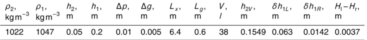
described above are presented in Carr and Davies (2006) and Carr et al. (2008). Here we consider in detail only one experiment, quoted under number 20538 (Carr and Davies, 2006). Its main parameters are given in Table 1 (the notation corresponds to Fig. 1).
3 Numerical model
25
NPGD
1, 1919–1946, 2014Features of fluid flows in strongly nonlinear internal
solitary waves
S. Semin et al.
Title Page
Abstract Introduction
Conclusions References
Tables Figures
◭ ◮
◭ ◮
Back Close
Full Screen / Esc
Printer-friendly Version
Interactive Discussion
Discussion
P
a
per
|
Discussion
P
a
per
|
Discussion
P
a
per
|
Discussion
P
a
per
the non-hydrodstatic system of fully nonlinear Navier–Stokes equations in the Boussi-nesq approximation (Marshall et al., 1997a). Both on the bottom and the left and right walls (Fig. 1), impermeable and slippage conditions (only the normal velocity to the boundary equals zero) are applied, while the upper boundary (fluid surface) is free. Viscosity is assumed turbulent (different horizontally and vertically), and given as an
5
additional item in the equation for the momentum:
D←
v=Ah
∂2v
∂x2+Av
∂2v
∂z2, (1)
wherev =v(u,w) is the velocity vector,Ah and Av are coefficients of horizontal and
vertical viscosity, which are implied as different (Table 2). The model also takes into ac-count the bottom friction (Adcroft et al., 2011) which is expressed by a greater viscosity
10
at the computed points located directly above the bottom. The additional term is
Guv-diss= rb+Cd q
2KE
!
∂2u
∂z2, (2)
whererb andCd are coefficients of linear and quadratic bottom friction, KE is the
av-erage kinetic energy at the computed bottom points. The itemGv-dissu (v-diss – vertical dissipation) is present only in the equation of the momentum conservation for the
hori-15
zontal component of the velocityu(x, z,t) above the bottom.
It should be noted that the value of the coefficient of eddy viscosity (Ah and Av,
respectively) and bottom friction (rbandCd) has a great influence on the magnitude of
the velocity field in the solitary wave. That is why the values of these parameters were chosen for a good consistency of laboratory and numerical results.
20
An additional diffusion item in the advection equation for the density in the numerical model MITgcm is taken into account:
Dρ=∇(K∇ρ) , whereK=
Kh 0
0 K
NPGD
1, 1919–1946, 2014Features of fluid flows in strongly nonlinear internal
solitary waves
S. Semin et al.
Title Page
Abstract Introduction
Conclusions References
Tables Figures
◭ ◮
◭ ◮
Back Close
Full Screen / Esc
Printer-friendly Version
Interactive Discussion
Discussion
P
a
per
|
Discussion
P
a
per
|
Discussion
P
a
per
|
Discussion
P
a
per
|
whereKis the diffusion tensor, which consists of the coefficients of the horizontal (Kh)
and vertical (Kv) diffusion (Table 2) taken from (Thiem et al., 2011).
Numerically the solitons are generated by the so-called gravitational collapse (Grue, 2005; Chen et al., 2007). Deviation from the average density in the model area is set as follows:
5
ρa(x,z)=∆ρ 2
tanhhz−zm−∆zp
2 th
x−L G m
i
/∆p, ∀x,z6∈(−h2∗+2∆p,−h2−2∆p);
−tanhx−LG
∆g
, ∀x,z6∈(−h∗2+2∆p,−h2−2∆p), (4)
where the first line sets the vertical profile of the density on the left and right of the gate, and the second – the horizontal profile on the site of the extracted gate;m=10−6m is a small value,h∗2=h2V +h2. In this, the jump on the free surface at the initial time is
given in the form of a step function:
10
ζ(x)= (
Hl−Hr, x≤Lg;
0, x > Lg.
(5)
The results of laboratory measurements and numerical simulations are shown below in a dimensionless form: xe=x/Lx, ze=z/h2 are horizontal and vertical coordinates, et=tc0/h2 is time, ζe=ζ /h2 is a free surface displacement, ηe=η/h2 is the vertical
displacement of the pycnocline, ue=u/c0 and we=w/c0 are horizontal and vertical
15
components of velocity correspondingly,c0=0.0974 m s
−1
is a characteristic speed of the internal wave propagation (this value is calculated from the linear theory of long waves for the given stratification),ωe=ω/Lxis the soliton width at half of the maximum value,ρe=ρ/ρref– the density normalized to its average valueρref=(ρ2+ρ1)/2. The
size of the spatial grid and the time step are as follows:∆x=0.0064 m,∆z=0.0013 m,
20
NPGD
1, 1919–1946, 2014Features of fluid flows in strongly nonlinear internal
solitary waves
S. Semin et al.
Title Page
Abstract Introduction
Conclusions References
Tables Figures
◭ ◮
◭ ◮
Back Close
Full Screen / Esc
Printer-friendly Version
Interactive Discussion
Discussion
P
a
per
|
Discussion
P
a
per
|
Discussion
P
a
per
|
Discussion
P
a
per
4 Analysis of the results
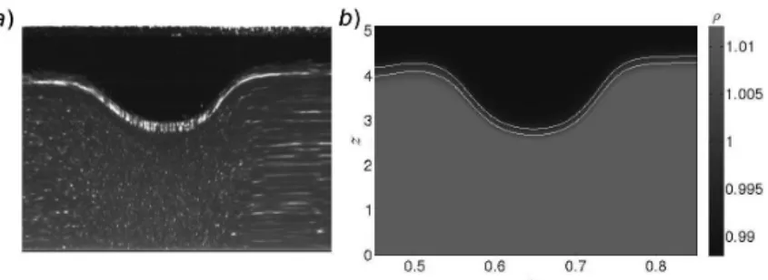
After a short transition period (t≈30, hereinafter the tilde symbol is omitted) a solitary
wave of negative polarity in the numerical tank is appeared. At the time momentt=
75.6 (the soliton center is located at the pointx=0.66) its shape is already fully formed (Fig. 2). Obviously, there is good agreement between the laboratory and the computed
5
waveform. The motion trajectories of an internal solitary wave in the pycnocline (η) and the perturbation of the free surface (ζ) are shown in Fig. 3 in the form ofx-tdiagrams. As seen from the Figure, the internal wave moves at a constant speed to the right boundary of the numerical tank, and then the wave is reflected from it. Weak lines corresponding to the dispersion packet, which follows the solitary wave and stretches
10
in time, can be seen in Fig. 3b.
It should be noted that if the polarity of the internal solitary wave in the thermocline is negative (as it is expected from theory), it manifests as a wave of elevation on the free surface (its amplitude is about 1 % of the amplitude of the wave in the pycnocline), as it follows from the linear and weakly nonlinear theory (Phillips, 1977).
15
On the surface, except the “footprint” of the internal wave (dark thick line in Fig. 3a), we can also see a rapidly propagating surface wave itself, which during the internal soliton nucleation time only runs to the right edge of the tank and back (thin line in Fig. 3a). It should also be noted that the description of the laboratory experiment (Carr and Davies, 2006) does not mention the surface effects, but they were probably present
20
in the tank. Since the amplitude of the surface displacement is very small, it has almost no effect on the internal dynamics of the internal soliton.
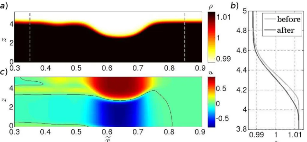
Figure 4a depicts the distribution of the fluid density at time t=75.6, as well as
the vertical density profile before and after the passage of the solitary wave (Fig. 4b). The change in the vertical profile of the density after the passage of the internal wave
25
NPGD
1, 1919–1946, 2014Features of fluid flows in strongly nonlinear internal
solitary waves
S. Semin et al.
Title Page
Abstract Introduction
Conclusions References
Tables Figures
◭ ◮
◭ ◮
Back Close
Full Screen / Esc
Printer-friendly Version
Interactive Discussion
Discussion
P
a
per
|
Discussion
P
a
per
|
Discussion
P
a
per
|
Discussion
P
a
per
|
the observed change is due either to a dispersing tail, or to nonlinear effects. It also shows the horizontal velocity field during the passage of the internal wave (Fig. 4c). As expected, the velocity below the trough is negative, and above is positive.The black curve in Fig. 4c, marks the contours of zero velocity. It is particularly necessary to note the presence of zero velocity contours in the bottom layer of the solitary wave, under
5
which the horizontal velocity takes a positive sign. In this layer called “the reverse flow” the fluid particles move in the same direction as the soliton. The detailed analysis of this effect is given in Sect. 6.
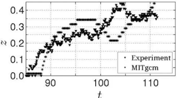
A more accurate comparison of the computed and experimental data is given in Fig. 5, which shows temporal variation of the pycnocline displacement at the fixed point
10
x=0.66. The results of computations in the framework of the Bergen Ocean Model
(BOM) (Thiem et al., 2011) are also presented. In both numerical models the computed amplitude exceeds the laboratory value by 14–15 % and correlates between them. However, the duration of the soliton-like wave in BOM is larger than in MITgcm, and this difference is due to different values of viscosity coefficients:AhBOM=5×10⁻⁵m2/c
15
andABOMv =1×10− 6
m2/c;AMITgcmh =5×10⁻⁴m2/candAMITgcmv =7.5×10− 6
m2/c. In fact, it was pointed in (Thiem et al., 2011) that the variation of viscosity coefficients can provide a better agreement with the laboratory data.
Both in the laboratory tank and in the numerical models the generated solitary wave is not symmetric about the centre of the trough. Its trailing edge is slightly swamped in
20
relation to the undisturbed pycnocline level (Figs. 2, 4 and 5), indicating the formation of the weak dispersive train behind the head wave due to the slight incompleteness of the process of soliton formation.
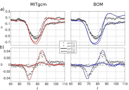
The comparative graphs of bottom vertical and horizontal velocities are shown in Fig. 6. The field of the horizontal velocity (Fig. 6a) is a bit better described by our
25
NPGD
1, 1919–1946, 2014Features of fluid flows in strongly nonlinear internal
solitary waves
S. Semin et al.
Title Page
Abstract Introduction
Conclusions References
Tables Figures
◭ ◮
◭ ◮
Back Close
Full Screen / Esc
Printer-friendly Version
Interactive Discussion
Discussion
P
a
per
|
Discussion
P
a
per
|
Discussion
P
a
per
|
Discussion
P
a
per
(Fig. 6a). As is noted in Thiem et al. (2011), this flow may occur at the balance of power bottom friction and pressure, leading to the separation of the bottom layer.
As for the vertical velocity, we can talk about the good agreement of both numerical models with laboratory measurements. We would like to note that the vertical velocity increases with the distance from the bottom, and it is natural in the bottom layer where
5
the condition of impermeability is applied on the bottom. However, it should be noted that in Thiem et al. (2011) a pronounced inflection point at the time of changing the sign of the vertical bottom speed is observed, while in our computations and in the laboratory experiment it is absent. This difference is explained by the fact that in Thiem et al. (2011) the soliton turned out to be wider than in our computations and is related
10
to the difference in the viscosity coefficients.
In general, the time series has four regions of the bottom layer: 1 – unperturbed state, 2 – the passage of the soliton, 3 – the reverse flow (the fluid particle movement is directed in the opposite direction of the velocity field of region 2), 4 – relaxation. These conditions are marked with numbers in Fig. 6a and are characterized directly
15
by the magnitude and sign of the velocity field over the selected point of the bottom surface.
It should be noted that both in the laboratory and in the numerical experiment (MIT-gcm) the reverse flow smooths the horizontal flow of the fluid in the soliton tail, so that the asymmetry, noticeable atz=0.6 is almost not visible at the pointz=0.1.
20
We determined the thickness of the reverse flow in the bottom layer as the distance from the bottom surface to the bottom contours of zero horizontal velocity (Fig. 4c). The evolution of the thickness of the reverse flow in the laboratory and numerical tanks
at the fixed point x=0.66 is shown in Fig. 7. As can be seen, the behavior of the
two curves is about the same, but there is a slight lag in the numerical model. If we
25
NPGD
1, 1919–1946, 2014Features of fluid flows in strongly nonlinear internal
solitary waves
S. Semin et al.
Title Page
Abstract Introduction
Conclusions References
Tables Figures
◭ ◮
◭ ◮
Back Close
Full Screen / Esc
Printer-friendly Version
Interactive Discussion
Discussion
P
a
per
|
Discussion
P
a
per
|
Discussion
P
a
per
|
Discussion
P
a
per
|
5 Comparison with the weakly nonlinear model
In the case of weakly nonlinear internal waves Euler equations can be asymptotically reduced to the extended version of the Korteweg–de Vries equation called the Gardner equation (Grimshaw et al., 2004, 2007, 2010):
∂η ∂t +
c+αη+α1η2 ∂η
∂x +β ∂3η
∂x3 =0, (6)
5
wherecis the speed of propagation of long internal waves,α andα1 are coefficients
of quadratic and cubic nonlinearities, respectively,βis the coefficient of dispersion. To calculate these coefficients it is necessary to determine the vertical structure of the mode, depending on the stratification of the fluid and its depth. In the case of the two-layer flow all the formulas are explicit (Grimshaw et al., 2002). In general, we have to
10
solve the problem of the Sturm–Liouville eigenvalue with zero boundary conditions on the fluid surface and bottom, see Holloway et al. (1999) and Grimshaw et al. (2007). Calculated in the Boussinesq approximation the coefficients are: α=−2.1 s−1, α1= −25.6 (m s)−1,β=1.9×10⁻⁴m3s−1.
Since the cubic nonlinearity coefficient is negative, there is only one family of solitons
15
described by the formula:
η(x,t)= A
1+Bcosh(γ(x−V t)),
A=a
2+aα1 α
, B=aα1
α +1, γ=
r
αa
6β
2+aα1 α
, V =βγ2, (7)
whereais soliton amplitude, varying from zero to the limiting value
alim=−α/α1=−0.081. (8)
20
NPGD
1, 1919–1946, 2014Features of fluid flows in strongly nonlinear internal
solitary waves
S. Semin et al.
Title Page
Abstract Introduction
Conclusions References
Tables Figures
◭ ◮
◭ ◮
Back Close
Full Screen / Esc
Printer-friendly Version
Interactive Discussion
Discussion
P
a
per
|
Discussion
P
a
per
|
Discussion
P
a
per
|
Discussion
P
a
per
calculated from Eq. (7)
ωg=2γarccosh
1
B+2
. (9)
The dependence of the width of the soliton on the relative amplitudea/alim, built by the
Eq. (9), is shown in Fig. 8.
In the fully nonlinear model the amplitude and width of the solitary wave varied by
5
changing the position coordinates of the gateLg and the volumeV of the added fluid,
while the density stratification practically does not change. Figure 8 shows the calcu-lated soliton width (with symbols) as a function of the amplitude normalized for con-venience to the same limiting amplitude of the Gardner soliton (Eq. 7). In the fully nonlinear model the limiting amplitude of the soliton is known only in the two-layer
10
stratification and is equal to Turner and Vanden-Broeck (1998)
alim=
hu−hl
2 =−0.083, (10)
wherehu=h2andhl=h1+δh1R are the heights of the upper and lower layers of the
fluid, respectively. This value is somewhat larger (in absolute value) than the limiting amplitude in the Gardner Eq. (7), but slightly less than in the limiting amplitude in the
15
fully nonlinear numerical model. In fact, the density stratification is not exactly a two-layer one (the thickness of the pycnocline is 20 % of the thickness of the upper two-layer), so the calculated maximum of the soliton amplitude is larger (dash-dotted vertical line in Fig. 8) than predicted by theory. The soliton width in the fully nonlinear model is also larger than in the Gardner model, if the amplitude of the soliton does not exceed the
20
NPGD
1, 1919–1946, 2014Features of fluid flows in strongly nonlinear internal
solitary waves
S. Semin et al.
Title Page
Abstract Introduction
Conclusions References
Tables Figures
◭ ◮
◭ ◮
Back Close
Full Screen / Esc
Printer-friendly Version
Interactive Discussion
Discussion
P
a
per
|
Discussion
P
a
per
|
Discussion
P
a
per
|
Discussion
P
a
per
|
6 The trajectories of Lagrangian particles
The measurements and calculations of the velocity field in the solitary wave are im-portant for calculating the sediment transport. As the first step to such a study, we compute the trajectories of Lagrangian particles. The traditional method of calculating the Lagrangian trajectories demands the solution of ordinary differential equations with
5
respect to the radius vector of the position of the particle in the velocity field (Lamb, 1997; Toschi and Bodenschatz, 2009):
dr
dt =v(r,t), r(t=0)=r0, (11)
wherer(t)={x(t),z(t)} is vector indicating the position of a particle at a given time, andr0={x0,y0}is the initial coordinates of the particle.
10
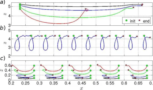
Figure 9 shows the calculated trajectory of Lagrangian particles located at the initial moment at the fluid surface, in the pycnocline and near the bottom. The largest particle displacement in the fluid in the horizontal direction is obtained at the surface and the direction of the movement coincides with the direction of the movement of the soliton (this is consistent with the positive sign of the horizontal velocity on the upper layer
15
above the soliton of the negative polarity, Fig. 4c). According to the calculations, the distance that the particle can go under the influence of the velocity field can be two and a half times larger than the width of the moving solitary wave. The direction of the movement of Lagrangian particles on the pycnocline (at the initial time located on the line of the unperturbed density) also coincides with the direction of motion of the
20
soliton, but the trajectories have a loop structure, since the vertical velocity prevails here, and the displacement does not exceed one-third the width of the wave. In the bottom layer the fluid particles move in the opposite direction (in line with the direction of the horizontal velocity) with a lesser amplitude of displacement than at the surface, which can be connected with a greater thickness of the lower layer and the damping of
25
NPGD
1, 1919–1946, 2014Features of fluid flows in strongly nonlinear internal
solitary waves
S. Semin et al.
Title Page
Abstract Introduction
Conclusions References
Tables Figures
◭ ◮
◭ ◮
Back Close
Full Screen / Esc
Printer-friendly Version
Interactive Discussion
Discussion
P
a
per
|
Discussion
P
a
per
|
Discussion
P
a
per
|
Discussion
P
a
per
trajectories are redirected to the positive side of the x axis. The magnitude of the
movement in the opposite direction does not exceed the half-width of the soliton. Notably, all the motion paths are not closed, as can be expected from theory for the wave of one polarity. However, some tendency to closeness is present at the bottom points where the reverse flow occurs.
5
The first analysis of the particle motion in an ideal fluid has been done in Lamb (1997) in the framework of the Euler equations and weakly nonlinear theory. The author con-sidered the movement of the particle only on the fluid surface, and we confirm his conclusion for the surface particles.
7 Conclusions
10
The features of the flow, induced by a strongly nonlinear solitary internal wave in a vis-cous two-layer fluid, are analyzed in the frame of this work. The soliton-like perturbation in the numerical model MITgcm is generated by the gravitational collapse method in a two-dimensional tank. The initial conditions are set on the basis of the laboratory experiment (Carr and Davies, 2006). The comparison of the computed results with the
15
laboratory measurements described in Carr and Davies (2006) is given. We also com-pare our results with the numerical results given in the frame of the Bergen Ocean
Model (Thiem et al., 2011). In our computations we used large (in one order) coeffi
-cients of viscosity than in Thiem et al. (2011). In both numerical models, the amplitudes obtained are 14–15 % higher than in the laboratory value. The solitary wave duration is
20
slightly different in both numerical models due to different values of the viscosity coef-ficients. The increase of these coefficients made in our computations leads to a better agreement with the observed soliton duration. Both numerical models also predict the reverse flow observed in the experiments. Our computations show that the moment of the appearance of the reversibility occurs with a short delay, and its thickness is no
25
NPGD
1, 1919–1946, 2014Features of fluid flows in strongly nonlinear internal
solitary waves
S. Semin et al.
Title Page
Abstract Introduction
Conclusions References
Tables Figures
◭ ◮
◭ ◮
Back Close
Full Screen / Esc
Printer-friendly Version
Interactive Discussion
Discussion
P
a
per
|
Discussion
P
a
per
|
Discussion
P
a
per
|
Discussion
P
a
per
|
The comparison of the parameters of solitary waves in a viscous fluid with the param-eters of the soliton in the Gardner equations in the weakly nonlinear theory of internal waves in an ideal fluid is also carried out. The calculated values of the limiting amplitude of solitons are larger than the similar values in the frame of the Gardner model. The width of the solitary waves in the fully nonlinear model is also larger than in the Gardner
5
model, if the amplitude of the soliton does not exceed the limiting value. We confirm the conclusion made in Michallet and Barthelemy (1998) about the similar difference in soliton width and amplitude.
The calculations of the trajectories of Lagrangian particles in the surface and in the bottom layers, as well as in the pycnocline are performed. The results demonstrated
10
completely different trajectories at different depths of the model area. Thus, the largest displacement of Lagrangian particles is observed in the surface layer, it can be more than two and a half times larger than the characteristic width of the soliton. Located at the initial moment along the middle of the pycnocline, fluid particles move along the vertically elongated loop at a distance of not more than one third of the width of
15
the solitary wave. In the bottom layer the fluid moves in the opposite direction of the internal wave propagation, but under the influence of the reverse flow, when the bulk of the velocity field of the soliton ceases to influence the trajectory, it moves in the opposite direction. The magnitude of displacement of fluid particles in the bottom layer is not more than the half-width of the solitary wave. Our results confirm the previous
20
results given in Lamb (1997) where the author investigated the dynamics of the surface particles only.
We conclude that the values of viscosity and bottom friction parameters have a criti-cal impact on the result. To achieve a better agreement of the laboratory and numericriti-cal experiments, it is necessary to vary them accordingly. This process takes a
consider-25
able amount of time and from a practical point of view is ineffective. Therefore, a direct method of measuring these values directly in experiments should be employed.
NPGD
1, 1919–1946, 2014Features of fluid flows in strongly nonlinear internal
solitary waves
S. Semin et al.
Title Page
Abstract Introduction
Conclusions References
Tables Figures
◭ ◮
◭ ◮
Back Close
Full Screen / Esc
Printer-friendly Version
Interactive Discussion
Discussion
P
a
per
|
Discussion
P
a
per
|
Discussion
P
a
per
|
Discussion
P
a
per
References
Adcroft, A. J., Campin, J., Dutkiewicz, S., Evangelinos, C., Ferreira, D., Forget, G., Fox-Kemper, B., Heimbach, P., Hill, C., Hill, E., Hill, H., Jahn, O., Losch, M., Marshall, J. S., Maze, G., Menemenlis, D., and Molod, A.: MITgcm User Manual, MIT Department of EAPS, Boston, 464 pp., 2011.
5
Apel, J. R., Ostrovsky, L. A., Stepanyants, Y. A., and Lynch, J. F.: Internal solitons in the ocean and their effect on underwater sound, J. Acoust. Soc. Am., 121, 695–722, 2007.
Berntsen, J.: Users Guide for a modesplitσ-coordinate numerical ocean model, University of Bergen, Bergen, 51 pp., 2004.
Bogucki, D. J. and Redekopp, L. G.: A mechanism for sediment resuspension by internal solitary 10
waves, Geophys. Res. Lett., 26, 1317–1320, 1999.
Cai, S., Long, X., and Gan, Z.: A method to estimate the forces exerted by internal solitons on cylindrical piles, Ocean Eng., 30, 673–689, 2003.
Cai, S., Wang, S., and Long, X.: A simple estimation of the force exerted by internal solitons on cylindrical piles, Ocean Eng., 33, 974–980, 2006.
15
Carr, M. and Davies, P. A.: The motion of an internal solitary wave of depression over a fixed bottom boundary in a shallow, two-layer fluid, Phys. Fluids, 18, 1–10, 2006.
Carr, M., Davies, P. A., and Shivaram, P.: Experimental evidence of internal solitary wave-induced global instability in shallow water benthic boundary layers, Phys. Fluids, 20, 1–12, 2008.
20
Chen, C.-Y., Hsu, J. R.-C., Chen, C.-W., Chen, H.-H., Kuo, C.-F., and Cheng, M.-H.: Generation of internal solitary wave by gravity collapse, J. Mar. Sci. Technol., 15, 1–7, 2007.
Cheng, M.-H., Hsu, J. R.-C., Chen, C.-Y., and Chen, C.-W.: Modelling the propagation of an internal solitary wave across double ridges and a shelf-slope, Environ. Fluid Mech., 9, 321– 340, 2008.
25
Chin-Bing, S. A., Warn-Varnas, A., King, D. B., Hawkins, J., and Lamb, K. G.: Effects on acous-tics caused by ocean solitons, Part B: Acousacous-tics, Nonlinear Anal.-Theor., 71, 2194–2204, 2009.
Donaldson, M. R., Cooke, S. J., Patterson, D. A., and Macdonald, J. S.: Cold shock and fish, J. Fish Biol., 73, 1491–1530, 2008.
30
NPGD
1, 1919–1946, 2014Features of fluid flows in strongly nonlinear internal
solitary waves
S. Semin et al.
Title Page
Abstract Introduction
Conclusions References
Tables Figures
◭ ◮
◭ ◮
Back Close
Full Screen / Esc
Printer-friendly Version
Interactive Discussion
Discussion
P
a
per
|
Discussion
P
a
per
|
Discussion
P
a
per
|
Discussion
P
a
per
|
Grimshaw, R., Pelinovsky, E., and Poloukhina, O.: Higher-order Korteweg–de Vries models for internal solitary waves in a stratified shear flow with a free surface, Nonlin. Processes Geophys., 9, 221–235, doi:10.5194/npg-9-221-2002, 2002.
Grimshaw, R., Pelinovsky, E. N., Talipova, T. G., and Kurkin, A. A.: Simulation of the transfor-mation of internal solitary waves on oceanic shelves, J. Phys. Oceanogr., 34, 2774–2791, 5
2004.
Grimshaw, R., Pelinovsky, E., and Talipova, T.: Modeling internal solitary waves in the coastal ocean, Surv. Geophys., 28, 273–298, 2007.
Grimshaw, R., Pelinovsky, E., Talipova, T., and Kurkina, O.: Internal solitary waves: propagation, deformation and disintegration, Nonlin. Processes Geophys., 17, 633–649, doi:10.5194/npg-10
17-633-2010, 2010.
Grue, J.: Generation, propagation, and breaking of internal solitary waves, Chaos, 15, 1–14, 2005.
Holloway, P., Pelinovsky, E., and Talipova, T.: A generalised Korteweg–de Vries model of internal tide transformation in the coastal zone, J. Geophys. Res., 104, 18333–18350, 1999.
15
Jackson, C. R.: An atlas of internal solitary-like waves and their properties, prepared under con-tract with the Office of Naval Research Code 322PO, Contract N00014-03-C-0176, Global Ocean Associates, 6220 Jean Louise Way Alexandria VA., 2004.
Helfrich, K. R. and Melville, W. K.: Long nonlinear internal waves, Annu. Rev. Fluid Mech., 38, 395–425, 2006.
20
Lamb, K. G.: Particle transport by nonbreaking, solitary internal waves, J. Geophys. Res., 102, 18641–18660, 1997.
Maderich, V., Talipova, T., Grimshaw, R., Pelinovsky, E., Choi, B. H., Brovchenko, I., Terlet-ska, K., and Kim, D. C.: The transformation of an interfacial solitary wave of elevation at a bottom step, Nonlin. Processes Geophys., 16, 33–42, doi:10.5194/npg-16-33-2009, 2009. 25
Maderich, V., Talipova, T., Grimshaw, R., Pelinovsky, E., Choi, B. H., Brovchenko, I., and Terlet-ska, K.: Interaction of a large amplitude interfacial solitary wave of depression with a bottom step, Phys. Fluids, 22, 076602, doi:10.1063/1.3455984, 2010.
Marshall, J. S., Hill, C., Perelman, L., and Adcroft, A. J.: Hydrostatic, quasi-hydrostatic, and nonhydrostatic ocean modeling, J. Geophys. Res., 102, 5733–5752, 1997a.
30
NPGD
1, 1919–1946, 2014Features of fluid flows in strongly nonlinear internal
solitary waves
S. Semin et al.
Title Page
Abstract Introduction
Conclusions References
Tables Figures
◭ ◮
◭ ◮
Back Close
Full Screen / Esc
Printer-friendly Version
Interactive Discussion
Discussion
P
a
per
|
Discussion
P
a
per
|
Discussion
P
a
per
|
Discussion
P
a
per
Michallet, H. and Barthélemy, E.: Experimental study of interfacial solitary waves, J. Fluid Mech., 366, 159–177, 1998.
Miyata, M.: Long internal waves of large amplitude, in: Nonlinear Water Waves, edited by: Horikawa, K. and Maruo, H., 399–406, Springer-Verlag, Berlin, 1988.
Ostrovsky, L. A. and Stepanyants, Y. A.: Do internal solitions exist in the ocean?, Rev. Geophys., 5
27, 293–310, 1989.
Ostrovsky, L. A. and Stepanyants, Y. A.: Internal solitons in laboratory experiments: comparison with theoretical models, Chaos, 15, 037111, doi:10.1063/1.2107087, 2005.
Phillips, O. M.: The Dynamics of the Upper Ocean, Cambridge University Press, 1977.
Shapiro, G. I., Shevchenko, V. P., Lisitsyn, A. P., Serebryany, A. N., Politova, N. V., and 10
Akivis, T. M.: Influence of internal waves on the suspended sediment distribution in the Pe-chora Sea, Dokl. Earth Sci., 373, 899–901, 2000.
Song, Z. J., Teng, B., Gou, Y., Lu, L., Shi, Z. M., Xiao, Y., and Qu, Y.: Comparisons of internal solitary wave and surface wave actions on marine structures and their responses, Appl. Ocean Res., 33, 120–129, 2011.
15
Stastna, M. and Lamb, K. G.: Sediment resuspension mechanisms associated with internal waves in coastal waters, J. Geophys. Res., 113, C10016, doi:10.1029/2007JC004711, 2008. Talipova, T., Terletska, K., Maderich, V., Brovchenko, I., Jung, K. T., Pelinovsky, E., and
Grimshaw, R.: Internal solitary wave transformation over the bottom step: loss of energy, Phys. Fluids, 25, 032110, doi:10.1063/1.4797455, 2013.
20
Thiem, Ø., Carr, M., Berntsen, J., and Davies, P. A.: Numerical simulation of internal soli-tary wave-induced reverse flow and associated vortices in a shallow, two-layer fluid benthic boundary layer, Ocean Dynam., 61, 857–872, 2011.
Toschi, F. and Bodenschatz, E.: Lagrangian properties of particles in turbulence, Annu. Rev. Fluid Mech., 41, 375–404, 2009.
25
Turner, R. E. L. and Vanden-Broeck, J.-M.: Broadening of interfacial solitary waves, Phys. Flu-ids, 31, 2486–2490, 1998.
Vlasenko, V., Stashchuk, N., and Hutter, K.: Baroclinic Tides: Theoretical Modeling and Obser-vational Evidence, Cambridge University Press, Cambridge, 351 pp., 2005.
Warn-Varnas, A., Chin-Bing, S. A., King, D. B., Hawkins, J., and Lamb, K. G.: Effects on acous-30
NPGD
1, 1919–1946, 2014Features of fluid flows in strongly nonlinear internal
solitary waves
S. Semin et al.
Title Page
Abstract Introduction
Conclusions References
Tables Figures
◭ ◮
◭ ◮
Back Close
Full Screen / Esc
Printer-friendly Version
Interactive Discussion
Discussion
P
a
per
|
Discussion
P
a
per
|
Discussion
P
a
per
|
Discussion
P
a
per
|
Table 1.Parameters of the laboratory experiment.
ρ2,
kg m−3
ρ1,
kg m−3
h2,
m
h1,
m
∆p, m
∆g, m
Lx, m
Lg, m
V,
l
h2V, m
δh1L, m
δh1R, m
Hl−Hr,
m
NPGD
1, 1919–1946, 2014Features of fluid flows in strongly nonlinear internal
solitary waves
S. Semin et al.
Title Page
Abstract Introduction
Conclusions References
Tables Figures
◭ ◮
◭ ◮
Back Close
Full Screen / Esc
Printer-friendly Version
Interactive Discussion
Discussion
P
a
per
|
Discussion
P
a
per
|
Discussion
P
a
per
|
Discussion
P
a
per
Table 2.The coefficients of diffusion, viscosity and the bottom friction.
Diffusion Viscosity Bottom friction
Kh Kv Ah Av rb Cd
NPGD
1, 1919–1946, 2014Features of fluid flows in strongly nonlinear internal
solitary waves
S. Semin et al.
Title Page
Abstract Introduction
Conclusions References
Tables Figures
◭ ◮
◭ ◮
Back Close
Full Screen / Esc
Printer-friendly Version
Interactive Discussion
Discussion
P
a
per
|
Discussion
P
a
per
|
Discussion
P
a
per
|
Discussion
P
a
per
|
Figure 1.The geometry of the laboratory experiment(a)before and(b)after extracting the gate
NPGD
1, 1919–1946, 2014Features of fluid flows in strongly nonlinear internal
solitary waves
S. Semin et al.
Title Page
Abstract Introduction
Conclusions References
Tables Figures
◭ ◮
◭ ◮
Back Close
Full Screen / Esc
Printer-friendly Version
Interactive Discussion
Discussion
P
a
per
|
Discussion
P
a
per
|
Discussion
P
a
per
|
Discussion
P
a
per
|
NPGD
1, 1919–1946, 2014Features of fluid flows in strongly nonlinear internal
solitary waves
S. Semin et al.
Title Page
Abstract Introduction
Conclusions References
Tables Figures
◭ ◮
◭ ◮
Back Close
Full Screen / Esc
Printer-friendly Version
Interactive Discussion
Discussion
P
a
per
|
Discussion
P
a
per
|
Discussion
P
a
per
|
Discussion
P
a
per
|
NPGD
1, 1919–1946, 2014Features of fluid flows in strongly nonlinear internal
solitary waves
S. Semin et al.
Title Page
Abstract Introduction
Conclusions References
Tables Figures
◭ ◮
◭ ◮
Back Close
Full Screen / Esc
Printer-friendly Version
Interactive Discussion
Discussion
P
a
per
|
Discussion
P
a
per
|
Discussion
P
a
per
|
Discussion
P
a
per
|
NPGD
1, 1919–1946, 2014Features of fluid flows in strongly nonlinear internal
solitary waves
S. Semin et al.
Title Page
Abstract Introduction
Conclusions References
Tables Figures
◭ ◮
◭ ◮
Back Close
Full Screen / Esc
Printer-friendly Version
Interactive Discussion
Discussion
P
a
per
|
Discussion
P
a
per
|
Discussion
P
a
per
|
Discussion
P
a
per
|