FACIAL FEATURE EXTRACTION USING
STATISTICAL
QUANTITIES OF CURVE COEFFICIENTS
SHREEJA R*
Student
Thadomal Shahani Engineering College Mumbai University
SHALINI BHATIA
Assistant Professor Computer Engineering Department Thadomal Shahani Engineering College
Mumbai University Abstract:-
Face recognition technology involves obtaining the identity of a person by comparing the image captured with the stored images in the database. In today’s world face recognition has relevance in many day to day applications. A large number of organizations are making use of various biometric techniques for applications such are employee sign in, access to secure systems etc. Unlike other biometric techniques it has the advantage that it can be done without the active participation of the person. So it can be extensively used in crime investigation purpose. For identifying faces the preliminary phase is to obtain the features of the faces which are crucial for recognition. In this paper a feature extraction method based on the statistical descriptors of Curve coefficients is proposed. Curvelet transform is a multiscale pyramid with many directions, positions at each length, scale, and needle shaped elements at fine scales. The Curvelet transform is an extension of wavelet originally designed to represent edges and other singularities along curves much more efficiently than traditional wavelet transforms. After curvelet transform, the coefficients of low frequency and high frequency in matrix form is obtained. The former contain the approximation of the face images, and we call them curve faces. The latter contain the detail information. The low frequency coefficients i.e. curve faces, contain most significant information of faces, and are crucial for recognition. But after curvelet transform a large number of coefficients are obtained. Using all these will make our recognition system complex. So the important features that are sufficient for recognition are to be extracted. In this paper a method of extracting the required features from the coefficients obtained after curvelet transform is discussed.
Keywords: Curve coefficients, Statistical quantities, Wavelet, Curvelet
I. Introduction
The Curvelet transform is a particular type of transformation that can be applied to the images to extract the edge discontinuities in the image. It is derived from the wavelet transformation. It is designed to represent edges and other singularities along curves much more efficiently than traditional wavelet transforms. In wavelet’s isotropic principle, the length and width of support frame is of equal size whereas in curvelet transform the width and length are related by the relation width ≈ length2 that is known as parabolic or anisotropic scaling.
we require all the details of the face image. Only the basic information will do. This is the idea behind curvelet transform. Curvelet represent the edges of an image.
2. Approaches & Feature Extraction Methods on still images
There are a number of factors which plays a crucial role in distinguishing one particular image from the other. They are related to the statistical and structural properties of the image. Analyzing and extracting those features have an important role in improving the efficiency of the detection system.
Feature extraction approaches on still images can be broadly grouped into geometric and template matching techniques. In the first case, geometric characteristics of faces to be matched, such as distances between different facial features, are compared. This technique provides limited results although it has been used extensively in the past. In the second case, face images represented as a two dimensional array of pixel intensity values are compared to a single or several templates representing the whole face. More successful template matching approaches use Principal Components Analysis (PCA) or Linear Discriminant Analysis (LDA) to perform dimensionality reduction achieving good performance at a reasonable computational complexity/time. Other template matching methods use neural network classification and deformable templates, such as Elastic Graph Matching (EGM) [3].
2.1 Principal Component Analysis (PCA)
The Principal Component Analysis (PCA) is one of the most successful techniques that have been used in image recognition and compression. PCA is a statistical method under the broad title of factor analysis. The purpose of PCA is to reduce the large dimensionality of the data space (observed variables) to the smaller intrinsic dimensionality of feature space (independent variables), which are needed to describe the data economically. This is the case when there is a strong correlation between observed variables [3].
The jobs which PCA can do are prediction, redundancy removal, feature extraction, data compression, etc. Because PCA is a classical technique which can do something in the linear domain, applications having linear models are suitable, such as signal processing, image processing, system and control theory, communications, etc. The main idea of using PCA for face recognition is to express the large 1-D vector of pixels constructed from 2-D facial image into the compact principal components of the feature space. This can be called Eigen space projection. Eigen space is calculated by identifying the Eigen vectors of the covariance matrix derived from a set of facial images (vectors) [3].
PCA computes the basis of a space which is represented by its training vectors. These basis vectors, actually eigenvectors, computed by PCA are in the direction of the largest variance of the training vectors. As it has been said earlier, we call them Eigen faces. Each Eigen face can be viewed a feature. When a particular face is projected onto the face space, its vector into the face space describes the importance of each of those features in the face. The face is expressed in the face space by its Eigen face coefficients (or weights). We can handle a large input vector, facial image, only by taking its small weight vector in the face space. This means that we can reconstruct the original face with some error, since the dimensionality of the image space is much larger than that of face space [3].
2.2 Linear Discriminant analysis (LDA)
2.3 Elastic graph matching (EGM)
Elastic graph matching is the basic process to compare graphs with images and to generate new graphs. In its simplest version a single labeled graph is matched onto an image. A labeled graph has a set of jets arranged in a particular spatial order. A corresponding set of jets can be selected from the Gabor-wavelet transform of the image. The image jets initially have the same relative spatial arrangement as the graph jets, and each image jet corresponds to one graph jet. The similarity of the graph with the image then is simply the average jet similarity between image and graph jets [3].
In order to increase the similarity one allows the graph to translate, scale and distort to some extent, resulting in a different selection of image jets. The distortion and scaling is limited by a penalty term in the matching cost function. The image jet selection which leads to the highest similarity with the graph is used to generate a new graph. When a bunch graph is used for matching, the procedure gets only a little bit more complicated. Besides selecting different image locations the graph similarity is also maximized by selecting the best fitting jet in each bunch. This is done independently of the other bunches to take full advantage of the combinatorics of the bunch graph representation [3].
3. Preprocessing Phase
The purpose of the pre-processing module is to reduce or eliminate some of the variations in face due to illumination. It normalizes and enhances the face image to improve the performance of the system. The preprocessing is crucial as the robustness of the system greatly depends on it. In this method histogram equalization is used for preprocessing the input image.
3.1 Histogram equalization
Histogram equalization is the most common histogram normalization or gray level transform, which purpose is to produce an image with equally distributed brightness levels over the whole brightness scale. It is usually done on too dark or too bright images in order to enhance image quality and to improve face recognition performance. It modifies the dynamic range (contrast range) of the image and as a result, some important facial features become more apparent [1].
The steps to perform histogram equalization are as follows:
1. For an N x M image of G gray-levels, create two arrays H and T of length G initialized with 0 values.
2. Form the image histogram: scan every pixel and increment the relevant member of H-- if pixel X has intensity p, perform H[p] = H[p] +1.
3. Form the cumulative image histogram Hc; use the same array H to store the result. H [O] = H [O]
H[p] = H [p -1] + H[p] For p = 1... G-1.
4. Set T[p] = (G-1/MN) H[p] (2)
Rescan the image and write an output image with gray-levels q, setting q = T[p].
The input images are histogram equalized. Histogram equalization process transforms the values in the color map so that the histogram of the gray component of the indexed image X is approximately flat. The mathematical notion is as follows:
ImgHisteq= T(X)
4. Curvelet Transform
To surmount the innate limitations of traditional multi-scale representations such as wavelet a novel transform has been developed by Candes and Donoho in 1999 known as curvelet transform. Curvelet transform is a multiscale pyramid with many directions, positions at each length, scale, and needle shaped elements at fine scales. The Curvelet transform is an extension of wavelet originally designed to represent edges and other singularities along curves much more efficiently than traditional wavelet transforms. In wavelet’s isotropic principle, the length and width of support frame is of equal size whereas in curvelet transform the width and length are related by the relation width ≈ length2 that is known as parabolic or anisotropic scaling [1].
The Curvelet transform is combination of Sub band Decomposition, Smooth Partitioning, Renormalization and Ridge let Analysis. Currently two implementations of Fast discrete Curvelet transform are available i.e. Unequi-Spaced Fast Fourier Transform based Curvelet and Frequency wrapping based Curvelet. The difference is the choice of spatial grid used to translate Curvelet at each scale and angle. Here the implementation selected to extract Curvelet coefficients is frequency wrapping based Curvelet. The Frequency wrapping based curvelet uses a decimated rectangular grid aligned with the image axes and for each given scale, there are two grids (decimated mostly horizontally or mostly vertically). Since no interpolation is necessary in the frequency plane, the transform is a numerical isometry and can be inverted by its ad joint [1].
After the histogram equalization phase, feature image is generated from Curvelet transform. Functionality-wise Curvelet transform can be written as
Curve_coeff = CT (s, Q, loc) (2)
Whereas s is scale parameter, Q is orientation parameter and loc is x, y spatial coordinates. The curve coefficients are generated at scale level 4 with 8 orientations. The statistical features of mean, standard deviation, skewness, entropy, and variance are calculated for each combination of scale and orientation. The smooth image is formed in order to reduce the ridges present in the image by taking norm between the input image and curve coefficients at scale 4, orientation 1. This smooth image is given as the input to the neural network [1].
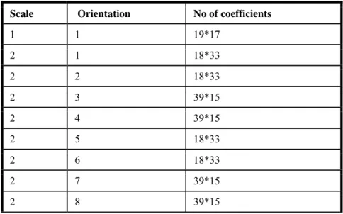
After curvelet transform, we get coefficients of low frequency and high frequency in matrix form. The former contain the approximation of the face images, and we call them curve faces. The latter contain the detail information. The low frequency coefficients i.e. curve faces, contain most significant information of faces, and are crucial for recognitionAfter computing the statistical features and smooth image coefficients; the formation of 1D feature factor is performed. This conversion method is called vectorization. This feature image can be used for face recognition [1].41 combinations of scale and orientation are obtained. The statistical quantities are obtained for each combination of scale and orientation. The obtained values are combined to form the feature vector. The organization of the coefficients obtained after curvelet transformation is shown in the table below.
Table 1. Results after Curvelet Transformation
Scale Orientation No of coefficients
1 1 19*17
2 1 18*33
2 2 18*33
2 3 39*15
2 4 39*15
2 5 18*33
2 6 18*33
“
Table 1 (Continued)”.Scale Orientation No of
coefficients
Scale Orientation No of coefficients
3 1 33*33 3 9 33*33
3 2 30*33 3 10 30*33
3 3 30*33 3 11 30*33
3 4 33*33 3 12 33*33
3 5 40*27 3 13 40*27
3 6 40*24 3 14 40*24
3 7 40*24 3 15 40*24
“Table 1 (Continued)”.
Scale Orientation No of coefficients Scale Orientation No of coefficients
4 1 66*66 4 9 66*66
4 2 60*66 4 10 60*66
4 3 60*66 4 11 60*66
4 4 66*66 4 12 66*66
4 5 80*54 4 13 80*54
4 6 80*49 4 14 80*49
4 7 80*49 4 15 80*49
4 8 80*54 4 16 80*54
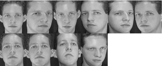
Fig. 1.Sample Image from ORL Database
4.1 Statistical Descriptors of Curve Coefficients
The feature extraction aspect of image analysis seeks to identify inherent characteristics or features of objects found within the image. These characteristics are used to describe the object. After doing curvelet transform a large number of curvelet coefficients are obtained. Not all coefficients are required for the detection of faces. So for feature extraction certain statistical descriptors are derived. A large number of statistical descriptors are available. They are mean, standard deviation, skewness, entropy, variance, norm, kurtosis or fourth moment etc. Each of these represents certain characteristics of the facial images which will be important for recognition. Statistical quantities are used to describe the texture of the image. Texture in images refers to variations in greylevel or color. If the grey level is constant everywhere in the object, the image has no texture. If the grey level varies significantly within the object, the object is said to have texture. The term texture generally refers to repetition of basic texture elements called texels. A texel contains several pixels, whose placement can be periodic or random. The statistical texture analysis characterizes textures as smooth, grainy, coarse etc. It uses statistical moments of the histogram of the image or the region.
5. Results and Discussions
Fig. 2.Block Diagram of the Proposed System
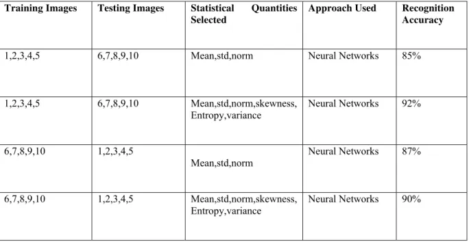
Table 2. Results of Recognition
Training Images Testing Images Statistical Quantities Selected
Approach Used Recognition
Accuracy
1,2,3,4,5 6,7,8,9,10 Mean,std,norm Neural Networks 85%
1,2,3,4,5 6,7,8,9,10 Mean,std,norm,skewness, Entropy,variance
Neural Networks 92%
6,7,8,9,10 1,2,3,4,5
Mean,std,norm
Neural Networks 87%
6,7,8,9,10 1,2,3,4,5 Mean,std,norm,skewness,
Entropy,variance
Neural Networks 90% Histogram
equalization
Curvelet Transform
Statistical quantitie
s
Input image
Feature Image
Train Neural Network
Test Neural Network
6. Conclusion
The proposed technique has used curvelet features for getting a compact representation of faces. The statistical feature extraction of the Curvelet coefficients and utilization of the coefficients in smoothing the input image has provided a feature set for face recognition. As more statistical descriptors are used the efficiency of detection will be improved. The main advantage is that as curvelet transform give the facial characteristics in different orientations, the angular deviation in the faces of individuals can also be represented. The angle of the face photograph will not affect the feature extraction and the detection process. So photos taken from different angles and different lighting conditions can be used for detection. The images can be captured by using any ordinary digital camera. So it is very cost effective also. The hardware and software requirements are also optimal.
Here Neural network method is used for recognition. Neural network has been found as an efficient method in many of the biometric techniques. It has the method of reducing the search space. Some of the images in the database are used for training and the rest are used for testing. As the number of images used for training increases the recognition efficiency is also increased. By using high speed systems with parallel processing capabilities this can be extended for a very large database. The main factor which affects the performance of the system is the time spent in training. But high speed or parallel processing systems can overcome this constraint as they can perform the training faster.
7. References
[1] Usman Qayyum, “Phase Efficient Neural Network using Curvelet Features for Face Recognition”, Proceedings of the 12th IEEE International Multitopic Conference, pp.:174-177, December 2008.
[2] Jiulong Z, Zhiyu Z, Wei H, Yanjun L, Yinghui W, “Face Recognition based on Curvefaces”, IEEE Third International Conference on Natural Computation , 2007.
[3] Shahrin Azuan Nazeer, Nazaruddin Omar, Marzuki Khalid, “Face Recognition System using Artificial Neural Networks Approach”, Signal Processing, Communications and Networking, pp.:420-425, Feb 2007.
[4] Yi -Chun Lee, Chin-Hsing Chen, “Face Recognition based on Digital Curvelet Transform”, Eighth International Conference on Systems Design and Applications, pp.:341-345, 2008.
[5] D. Beymer, “Face recognition under varying pose”, IEEE Conference on Computer Vision and Pattern Recognition, pp.: 756–761, 1994. [6] Jean-Luc Starck, Emmanuel J. Candès, David L. Donoho, “The Curvelet Transform for Image Denoising,”, IEEE Transactions on image