Solutions of Maximal Compatible Granules and Approximations in Rough Set Models

(1)

Available Online at 111_.ijecse_.org ISSN: 2277-1956

Solutions of Maximal Compatible Granules

and Approximations in Rough Set Models

Chen Wu, Dandan Li, Lijuan Wang ,Wei Xu, Xibei Yang

Jiangsu University of Science and Technology Zhenjiang, Jiangsu, 212003, P.R. China

Abstract—This paper emphasizes studying on a new method to rough set theory by obtaining granules with maximal compatible classes as primitive ones in which any two objects are mutually compatible, proposes the upper and lower approximation computations to extend rough set models for further building multi-granulation rough set theory in incomplete information systems, discusses the properties and relationships of granules and approximations, designs algorithms to solve maximal compatible classes, the lower and upper approximations. It verifies the correctness of algorithms by an example.

Keywords- incomplete information system; rough set model; maximal compatible class; algorithm; multi-granulation

I. INTRODUCTION

In 1982s, Pawlak put forward rough set theory (RST for short) [1], which are applied in many scientific and technological areas such as Data Mining, Pattern Recognition, Knowledge Acquisition, Machine Learning, Intelligent Decision and so on, as an extension of set theory for studying intelligent systems [2],[3] characterized by uncertainty and imprecision. It is for complete information systems. Indiscernibility relation is the main relation. But in incomplete information systems (IIS for short), it is not always possible to build an indiscernibility relation due to that the existence of null or missing attribute values..

Now a new trend to deal with knowledge acquisition problems in IIS is to form non-indiscernibility relation such as tolerance relation suggested by M. Kryszkiewicz, similarity relation put forward by J.Stefanowski [4],[5]. limited tolerant relation proposed by W.Guoying [6], and so on [7].

The present paper puts forward a new granule view with maximal compatible class as primitive granules based on tolerance relation to promote the model to handle IIS. It brings even a new expect to produce a new approach for transacting multi-granulation RST problems in IIS. The main task of it is to analyze and design a series of granules and related algorithms for forming approximations and then using them to acquire exact knowledge from massive data systems conveniently and efficiently. So the work done here is of necessary and helpful.

II. DEFINITIONS

An IIS is a quadruple

S

=

( ,

O AT V f

, , )

([4]). The tolerance relation derived by

A

⊆

AT

is defined as:

( )

{( , )

:

,

_a

( )

_a

( )

_a

( )

*

_a

( )

*}.

T A

=

x y

∈ ×

U U

∀ ∈

a

A f x

=

f

y

∨

f x

= ∨

f

y

=

Tolerance class for

x

respecting to

A

⊆

AT

is

T x

_A

( ) {

= ∈

y O x y

:( , )

∈

T A

( )}

.

O T A

/ ( ) { ( ) |

=

T x x O

_A

∈

}

constructs a

cover on

U

,

called tolerance class space or quotient space.

T X

_A

( ) {

= ∈

x O T x

:

_A

( )

∩ ≠ ∅

X

}

is the upper

approximation, and

T X

_A

( ) {

= ∈

x O T x

:

_A

( )

⊆

X

}

the lower one, for

X

⊆

O

,.

Definition 1. Let

x

∈

O

,

A

⊆

AT

.

The compatible class(es) containing

x

is defined as 2

( )

max{

:

,

( )}

A

C

x

=

X x

∈

X X

⊆

T A

where max means operation is acting on by operator

⊆

.

C

_A

( )

x

may be not unique.

Definition 2. Let

A

⊆

AT

.

C A

( )

defined as a compatible knowledge expression system, where,

2

( ) {

: max{

( )}}.

C A

=

X

⊆

O

X

⊆

T A

Definition 3. the upper and lower approximations for

X

⊆

O

in knowledge system

C A

( )

are defined as follows:

( ),

( )

A _{Y C A X} _Y

(2)

III. PROPERTIES AND RELATIONSHIPS

Theorem 1.

X

∈

C A

( )

if and only if

X

= ∩

T y

_A

( ){

y

∈

X

}

.

Proof. Let

X

∈

C A

( )

. Then for any

x z

,

∈

X

,

( , )

x z

∈

T A x

( ),

∈

T z

_A

( )

So

x

∈∩

_{y X}_∈

T y

_A

( )

and

( ){

}.

A

X

⊆ ∩

T

y

∈

X

On the other hand, let

z

∈∩

T y

_A

( ){

y

∈

X

}

be any given, then

z

∈

T y

_A

( )

for any

y

∈

X

.That

z

is compatible with any element in

X

.

Because

X

∈

C A

( ),

X

⊆ ∪

X

{ }

z

and

X

is

maximal compatible class, it must have

z

∈

X

,other wise

X

∪

{ }

z

is a compatible class included in another maximal

one. That contradicts to

X C A

∈

( ).

Thus

∩

T y y X

A

( ){

∈ ⊆

}

X

.

Therefore

X

=∩

T y y X

A

( ){

∈

}.

When

X

= ∩

T y

A

( ){

y

∈

X

}

, for any

w z

,

∈

X

=∩

T y y X

A

( ){

∈

}

, we have

( , )

z w

∈

T A

( ),

for

( ),

( )

A A

w T z z T w

=

∈

.Thus

X

× ⊆

X

T A

( )

. So

X

is a compatible class. Now we prove that

X

is also a maximal

compatible class. If there is a q

∉

X such that

(

X

∪

{ })

q

2

⊆

T A

( )

, then

q T x

∈

_A

( )

for any

x

∈

X

. Then

( ){

}

.

A

q

∈∩

T y

y

∈

X

=

X

That is a contradiction. Therefore

X

is maximal. Synthesizing the two directions, the theorem holds.

Property 2.

( ) ( ) ( )

( )

A A

A

Y C A Y T x X C x

T x

Y

X

∈ ∧ ⊆ ∈

=

∪

= ∪

Proof. It is clear that

( ) P( )

( )

P Y C P∈

∪

∧ ⊆Y T x

Y

⊆

T x

.Now we prove

( ) ( )

( )

A A

Y C A Y T x

T x

Y

∈ ∧ ⊆

⊆

∪

. For

∀ ∈

z T x

_P

( ),

there must exists

an

X

∈

C P

( )

such that

{ , }

x z

⊆

X

.

Thus all element in

X

is compatible with

x

, so

X

⊆

T x

P

( )

.

Therefore,

( ) ( )

{ , }

.

P Y C P Y T x

x z

X

Y

∈ ∧ ⊆

⊆ ⊆

∪

So

( ) _P( )

.

Y C P Y T x

z

Y

∈ ∧ ⊆

∈

∪

Furthermore,

( ) ( )

( )

.

P P

Y C P Y T x

T x

Y

∈ ∧ ⊆

⊆

∪

we have

( ) ( )

( )

.

P P

Y C P Y T x

T x

Y

∈ ∧ ⊆

=

∪

For

X C x

∈

_A

( )

, we have

X

⊆

T x

_P

( )

, thus

( )

( ).

P

P X C x∈

∪

X T x

⊆

For

∀ ∈

z T x

_P

( )

,there exists a

Y C x

∈

_P

( )

，Such that

{ , }

x z

⊆

Y

, so

z

∈ ⊆

Y

( ) P

X C∈

∪

x

X

.This means

T x

P

( )

⊆ ∪

X C x∈_P( )

X

. Therefore,

T x

P

( )

= ∪

X C x∈_P( )

X

.Thus

( ) ( ) ( )

( )

P P

P

Y C P Y T x X C x

T x

Y

X

∈ ∧ ⊆ ∈

=

∪

= ∪

.

Theorem 2. Let

P Q

,

⊆

AT

.

For

∀ ∈

x

O

,

T x

_Q

( )

=

T x

_P

( )

if, and only if

C P

( )

=

C Q

( ).

The proof is omitted here.

Theorem 3. Let

P Q

,

⊆

AT

.

For

∀ ∈

x

O

,

T x

_Q

( )

=

T x

_P

( )

if, and only if

C

_P

( )

x

=

C

_Q

( ).

x

The proof is omitted here.

IV. ALGORITHMS AND AN EXAMPLE

A. Finding maximal compatible class algorithm

Let

O

=

{ |

x i

_i

=

1, 2,..., }

n

. We use

M

=

(

m

_{ij n n}

)

_× , where

m

_ijequals 1, if

( ,

x x

_i _j

)

∈

T A

( )

, 0 otherwise as adjacent matrix and .a 2-dimensional binary matrix

P

_{m n}_× , where

P v j

( , ) 1

=

means that

x

_j belongs to the v-th maximal compatible class,

P v j

( , )

=

0

means not, v=1,2,…,k, to store all maximal compatible classes, where

m

<=

( * ) / 2

n n

, but

m may be greater than n in some cases. Suppose there are totally

k

maximal compatible classes. After finishing computation, they are stored in the first

k

rows of

P

_{m n}_× .

Algorithm description

Input matrix M,n--number of U; Initialization: Pm×n<=0，counter k<=-1 Description :

for ( j=n-2;j>=0 ,j--) for (i=n-1 ;i> j-1,i--) { if (M[i, j]==1)

(3)

for (u=0,u<K-1;u++)

if (P[u,i]==1) // xi in u-th class { tag=1; //full compatible check for( v=j ;v<n ,v++)

if(!(P[u,v]==1&&M[v,j]==1) {tag=0; break;}

if(tag==1) P[u,j]=1; else //to form anew one for (v=j ;v<n;v++)

if (P[u,v]==1&&M[v,j]==1) {P[k,v]=1;break;}

// xj partial compatible in u-th class }

} }

for(v=0 ;v<k;v++)

for (v0=0;v0<k-1;v++) if (v0!=v)

{ tag=1;

for (u=0 ;u< n ;u++) if(P[v,u]==1)

if (P[v0,u]==1) continue; else

{ tag=0;break;} if (tag==1 )

for (u=0;u< n ;u++) P[v,u]=0; //erase redundant class }

// the following finds singleton class for(i=0;i<n;i++)T[i]=0; // T is a temporary array for( i=0,i<n;i++)

for (r=0 r<k ;r++) T[i]=T[i]+P[r][i]; for( i=0;i<n;i++)

if(T[i]==0) {k=k+1; P[k, i]=1;}

Output: Pm×n，the first k rows of it store all maximal compatible classes.

The synchronistic time complexity is

O n

(

3

)

.

B. Finding upper Approximation algorithm

After getting maximal compatible class matrix Pm×n , we can find upper approximation according to relative

definition. Let

X

⊆

O

. In order to compute

C X

A

( )

from

C A

( )

easily,

X

⊆

O

is represented by an array

X[0..n-1],where X[i]=1 if

u

_i₊₁

∈

O

and X[i]=0 otherwise, i=0,1,…,n-1.n=|O|.

Input: P, array X, k;

Initialization: array T: for(i=0;i<n;i++) T[i]=0; Description:

for(u=0; u<k;u++)

// check the u-th class including in X or not. { tag=1;

for( i=0;i<n;i++)

if(P[u][i]*X[i]==1) {tag=0;break;} if (tag==0)

for(i=0;i<n;i++) if (P[u][i]==1) T[i]=1; }

(4)

C. Finding lower Approximation algorithm

Let

X

⊆

O

. This algorithm finds out the lower approximation

C

_A

( )

X

in

C A

( )

.In order to compute easily, X is

represented by an array X[0..n-1],where X[i]=1 if

u

_i₊₁

∈

U

and X[i]=0 otherwise, i=0,1,…,n-1.n=|U|.

Input: P, X, k;

Initialization: array T: for( i=0;i<n;i++) T[i]=0; Description:

for(u=0;u<k;u++) { tag=1;

for (i=0;i<n;i++) if (P[u][i]==1)

if(X[i]==0) {tag=0;break;} if (tag==1) T[u]=1;

}

Output: T, the lower approximation of X. The synchronistic time complexity is O(kn).

V. AN EXAMPLE

In order to analyze comparatively, we adopt a real incomplete information system in [5] shown in TABLE 1 to

perform only computations of

C X

_A

( )

and

C

A

( )

X

for

X

⊆

O

.

where

AT

=

{ , , , },

a b c d

and

O

=

{ |

O i

i

=

1,2,...,12}

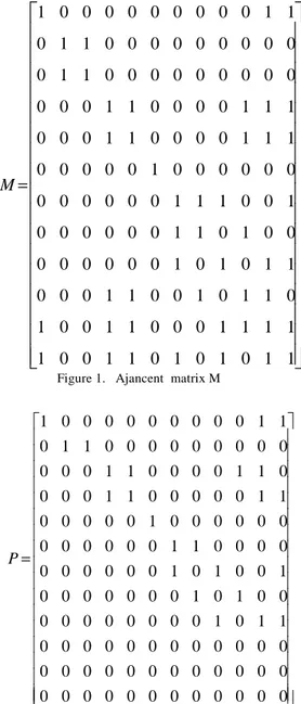
. e

is a decision attribute. Let A=AT. The adjacent matrix M representing the tolerance relation is shown in Figure 1.

The matrix P storing maximal compatible classes is in Figure 2.From Figure 2, we obtain that

C A

( )

contains

following maximal compatible classes:

{ ,

O O O

₁ ₁₁

,

₁₂

},

{ ,

O O

2 3

},

{ ,

O O O O

4 5

,

10

,

11

},

{ , ,

O O O O

4 5 11

,

12

},

6

{

O

},

{ , },

O O

₇ ₈

{ ,

O O O

₇ ₉

,

₁₂

},{ ,

O O

₈ ₁₀

},

{ ,

O O O

₉ ₁₁

,

₁₂

}

.

The decision classes of TABLE 1 are

D

=

{

O

,

O O O O O

, , ,

,

}

,

D

=

{ , , , , ,

O O O O O O

}

.

U a b c d e

O1 3 2 1 0 Φ

O2 2 3 2 0 Φ

O3 2 3 2 0 Ψ

O4 * 2 * 1 Φ

O5 * 2 * 1 Ψ

O6 2 3 2 1 Ψ

O7 3 * * 3 Φ

O8 * 0 0 * Ψ

O9 3 2 1 3 Ψ

O10 1 * * * Φ

O11 * 2 * * Ψ

O12 3 2 1 * Φ

(5)

Let

X

₁

=

D

_Φ. We compute upper and lower approximations of X according to their algorithms B and C, respectively. At first we represent or encode X1 into an array (1,1,0,1,0,0,1,0,0,1,0,1),then compute

C

A

(

X

1

)

and

C

A

(

X

1

)

. In

calculating

C

A

(

X

₁

)

, we get T=(0,0,0,0, 0,0,0,0,0,0,0,0), so

C

A

(

X

1

)

= ∅

. In calculating

C

A

(

X

1

)

, we get T =

(1,1,1,1,1,0,1,1,1,1,1,1), so,

C

A

(

X

₁

)

=

O

−

{

O

6

}

.

1 0 0 0 0 0 0 0 0 0 1 1

0 1 1 0 0 0 0 0 0 0 0 0

0 0 0 1 1 0 0 0 0 1 1 1

0 0 0 0 0 1 0 0 0 0 0 0

0 0 0 0 0 0 1 1 1 0 0 1

0 0 0 0 0 0 1 1 0 1 0 0

0 0 0 0 0 0 1 0 1 0 1 1

0 0 0 1 1 0 0 1 0 1 1 0

1 0 0 1 1 0 0 0 1 1 1 1

1 0 0 1 1 0 1 0 1 0 1 1

M

=













































































Figure 1. Ajancent matrix M

1 0 0 0 0 0 0 0 0 0 1 1 0 1 1 0 0 0 0 0 0 0 0 0 0 0 0 1 1 0 0 0 0 1 1 0 0 0 0 1 1 0 0 0 0 0 1 1 0 0 0 0 0 1 0 0 0 0 0 0 0 0 0 0 0 0 1 1 0 0 0 0 0 0 0 0 0 0 1 0 1 0 0 1 0 0 0 0 0 0 0 1 0 1 0 0 0 0 0 0 0 0 0 0 1 0 1 1

0 0 0 0 0 0 0 0 0 0 0 0 0 0 0 0 0 0 0 0 0 0 0 0 0 0 0 0 0 0 0 0 0 0 0 0

P

 

 

=_ _

 

 

Figure 2. Matrix P

Let

X

₂

=

D

_Ψ . Encode X2 into an array (0,0,1,0, 1,1,0,1,1,0,1,0), then compute

C

A

(

X

2

)

and

C

A

(

X

2

)

. In calculating

C

_A

(

X

₂

)

, we get T=(0,0, 0,0,0,1,0, 0,0,0,0,0), so

C

_A

(

X

₂

)

=

{

O

₆

}

. In calculating

C X

_A

(

₂

)

, we get

T=(1,1,1,1,1,1,1,1,1,1,1,1), so,

C

_A

(

X

₂

)

=

O

.

VI. APPLICATIONS IN MULTI-GRANULATION MODEL

(6)

we can introduce them into multi-granulation rough set Using knowledge expression systems

C A

( )

, we can also obtain related new research results.

Let

A A

₁

,

₂

,...,

A

_m

⊆

AT

be

m

attribute subsets. Then for

∀ ⊆

X

O M

,

=

{1, 2,..., }

m

, the optimistic

multi-granulation lower and upper approximations of

X

with respect to

A A

₁

,

₂

,...,

A

_mare defined respectively as:

1

( )

(

( ) (

)))

o m

i i

i=

A X

=∪ ∃ ∈

Y i M Y C A

∈

∧ ⊆

Y

X

∑

₁

( ) ~

₁

(~

)

o

m _o m

i i

i=

A

X

=

i=

A

X

∑

The optimistic multi-granulation boundary region of

X

is

1 1 1

( )

( ).

m Ai i

o

m m

o o

i i

Bn

X

A

X

A

X

∑₌

=

∑

=

−

∑

=

The pessimistic multi-granulation lower and upper approximations respectively are:

1

( )

(

( )

))

p

m

i i

i=

A

β

X

= ∪ ∀ ∈ ∃ ∈

Y

i M Y C A

∧ ⊆

Y

X

∑

1

( ) ~

1

(~

)

p

m _p m

i i

i=

A

β

X

=

i=

A

β

X

∑

The pessimistic multi-granulation boundary region of

X

is

1 1 1

( )

( ).

m Ai i

p

m m

p p

i i

Bn

X

A

X

A

X

∑₌

=

∑

=

−

∑

=

Using Finding maximal compatible class algorithm as a basic to find all

C A

(

_i

)

in

A

_i(

M

=

{1, 2,..., })

m

, we can not

hardly design related algorithms to compute lower and upper approximations of a given subset in optimistic multi-granulation and pessimistic multi-multi-granulation rough set models.

VII. CONCLUSIONS

Using maximal compatible classes as primitive granules, this paper defines

C A

( )

as a knowledge representing system. It extends original rough set model to a generalized one. Algorithms to solve maximal compatible classes, upper and lower approximations are suggested through binary matrices at some advantages. The correctness of the algorithms is verified by experiments through programming and execution on computers on several data sets. It provides a new forming granule view to solve problems in rough set model in dealing with incomplete information systems. This novel granular approach leads to increasing study methods in multi-granulation rough set models.

REFERENCES

[1] Z.Pawlak, “Rough sets and intelligent data analysis”, Information Sciences. 147 (2002) ,pp.1-12.

[2] W.Roman, Q.Swiniarski and A.Skowron, “Rough Set Method in Feature Selection and Recognition”, Pattern Recognition Letters, 24 (2003),pp. 833~849.

[3] J.S.Mi,W.Z.Wu and W.X.Zhang, “Approaches to Knowledge Reduction Based on Variable Precision Rough Set Model”, Information Sciences. 159 (2004),pp.255-272.

[4] M.Kryszkiewicz, “Rough Set Approach to Incomplete Information Systems”,Information Sciences, 112 (1998), pp.39-49. [5] J.Stefanowski, “Incomplete Information Tables and Rough Classification”,J. Computational Intelligence. 17 (2001),pp.545-566.

[6] W.L.Chen,J.X.Cheng and C.J.Zhang, “A Generalization to Rough Set Theory Based on Tolerance Relation”, J. computer engineering and applications, 16(2004),pp. 26-28.

[7] C.Wu, X.B.Yang, “Information Granules in General and Complete Covering”, Proceedings of the 2005 IEEE International Conference on Granular Computing, pp. 675-678.

[8] Qian Y H, Liang J Y, Yao Y Y, C, et al, “MGRS: a multigranulation rough set”, Information Sciences, 2010,vol.180,no.6,pp.949–970

[9] Qian Y. H, Liang J. Y, Dang C Y. “Incomplete multigranulation rough set”, IEEE Transactions on Systems, Man and Cybernetics, Part A, 2010,vol.40,no.2,pp. 420-431.