CHAOS THEORY APPLIED TO INPUT SPACE REPRESENTATION OF
AUTONOMOUS NEURAL NETWORK-BASED SHORT-TERM LOAD
FORECASTING MODELS
Vitor Hugo Ferreira
∗ [email protected]Alexandre Pinto Alves da Silva
† [email protected]∗Electrical Engineering Department, Fluminense Federal University (UFF) Rua Passo da Pátria, 156, Sala 509, Bloco D
CEP 24210-240 – Niterói RJ
†Electrical Engineering Program, PEE-COPPE, Federal University of Rio de Janeiro (UFRJ)
P.O. 68504
CEP 21945-972 – Rio de Janeiro RJ
RESUMO
Teoria do Caos Aplicada à Definição do Conjunto de En-tradas de Modelos Neurais Autônomos para Previsão de Carga em Curto Prazo
Após 1991, a literatura sobre previsão de carga passou a ser dominada por propostas baseadas em modelos neurais. En-tretanto, um empecilho na aplicação destes modelos reside na possibilidade do ajuste excessivo dos dados, i.e, overfitting. O excesso de não-linearidade disponibilizado pelos mode-los neurais de previsão de carga, que depende da represen-tação do espaço de entrada, vem sendo ajustado de maneira heurística. Modelos autônomos incluindo técnicas automáti-cas e acopladas para seleção de entradas e controle de com-plexidade dos modelos foram propostos recentemente para previsão de carga em curto prazo. Entretanto, estas técnicas necessitam da especificação do conjunto inicial de entradas que será processado pelo modelo visando determinar aquelas mais relevantes. Este trabalho explora a teoria do caos como ferramenta de análise não-linear de séries temporais na defi-nição automática do conjunto de atrasos de uma dada série de carga a serem utilizados como entradas de modelos neurais
Artigo submetido em 03/03/2011 (Id.: 01285) Revisado em 06/05/2011, 14/08/2011
Aceito sob recomendação do Editor Associado Prof. Carlos Roberto Minussi
autônomos. Neste trabalho, inferência Bayesiana aplicada a perceptrons de múltiplas camadas e máquinas de vetores re-levantes são utilizadas no desenvolvimento de modelos neu-rais autônomos.
PALAVRAS-CHAVE: Previsão de carga, Redes Neurais Ar-tificiais, Seleção de Entrada, Teoria do Caos, Sincronização caótica, Inferência Bayesiana, Perceptron de Multi-camadas , Máquinas de Vetores Relevantes.
ABSTRACT
set that will be processed by the model in order to select the most relevant variables. This paper explores chaos theory as a tool from non-linear time series analysis to automatic se-lect the lags of the load series data that will be used by the neural models. In this paper, Bayesian inference applied to multi-layered perceptrons and relevance vector machines are used in the development of autonomous neural models.
KEYWORDS: Load Forecasting, Artificial Neural Networks, Input Selection, Chaos Theory, Chaotic Synchronization, Bayesian Inference, Multi-layered Perceptron, Relevance Vector Machines.
1
INTRODUCTION
The decision making process in power systems, including economic dispatch, hydrothermal coordination, automatic generation control, energy trading and so on, requires the knowledge of the future behavior of the load dynamics. Along the last two decades, many load forecasting models have been proposed, with the neural network based mod-els receiving great attention. This is because they have been showing superior prediction performance, specially for short-term applications (Hippert, et. al., 2001). In fact, the neural network based models have been presenting outstand-ing results for multivariate problems envolvoutstand-ing databases with huge cardinality, as the short-term load forecasting problem (Ferreira and Alves da Silva, 2007), (Ferreira and Alves da Silva, 2009) and (Ferreira and Alves da Silva, 2010). Even been more robust than traditional models, criti-cal questions like input space representation and complexity control of neural network have not received the necessary at-tention.
The input selection stage is the one of the most important tasks in the development of load forecasting models. Feature extraction via non-linear techniques like wavelets uses only information about the time-series to be predicted without di-rect concern with the forecasting accuracy. In this sense, an input selection methodology directly related with the neural network model is required. The methods that use the model itself in the input selection step are called wrapper methods, and the ones that consider only the dynamics and statistics of the time-series are called filter methods (Guyon and Elis-seeff, 2003). For forecasting purposes, the wrapper methods are more indicated since these techniques aim to select the inputs that are most sutiable to the model in terms of fore-casting performance.
The complexity control of neural models has the objective of adjusting the non-linear extent of the neural network to the regularity exhibited by the data. This step is necessary to avoid the harmful modeling of the noisy component of the data, named overfitting. This can compromise the
general-ization capacity of the neural model, i.e., good predictions for unseen data.
Autonomous neural forecasting models, including automatic input selection, complexity control and structure selection, are necessary to reduce the necessity of intervention from ex-perts. These automatic procedures allow the extension of the forecasting to the bus load level. Autonomous Neural Net-work Load Forecasting models have been proposed in the literature (Ferreira and Alves da Silva, 2007) using Bayesian Inference Applied to Multi-Layered Perceptrons (BIAMLPs) and Support Vector Machines (SVMs) training and specifica-tion. These procedures include automatic and coupled proce-dures for input selection, complexity control and model spec-ification. However, these procedures still require the defini-tion of an initial set of inputs.
In order to improve the autonomous capability of the models proposed in (Ferreira and Alves da Silva, 2007), techniques for automatic definition of the initial set of inputs from the available time-series are necessary. This paper investigates the application of Chaos Theory as a tool for automatic def-inition of the initial set of inputs to be used with the au-tonomous neural models proposed in (Ferreira and Alves da Silva, 2007). The BIAMLPs are used in this paper and they are compared with Relevance Vector Machines (RVMs). Be-ing a sparse kernel model, a RVM can be seen as a SVM de-rived from the application of Bayesian Inference. The fore-casting performance of the models are compared using three public load and temperature databases. The main contribu-tions of the paper can be summarized as follows:
a) proposal of an automatic method for selecting inputs of neural network load forecasting models, based on time-series and calendar information, only; and
b) evaluation of the applicability of RVMs to the load fore-casting problem.
This paper is organized as follows. In Section 2, Chaos The-ory is presented in the context of Input Space Reconstruction. BIAMLPs are described in Section 3. Section 4 is devoted to the description of the RVMs. The database description and results are shown in Section 5. The discussion, main conclu-sions and future work are presented in Section 6.
2
CHAOS THEORY
The Chaos Theory development is motivated by the study of dynamical systems sensitive to initial conditions. After the transient effects, a dynamical system F(X) : RD → RD
X(k+ 1) =F[X(k)] (1)
From the actual stateX(k), all of the adjacent states of the deterministic system described by equation (1) can be ob-tained. The sensitivity to the initial conditions makes the trajectory of the system dependent on the knowledge of the functionF(X)and the value of the initial state. The set of initial conditions that drives asymptotically the system to a given region of the space is called basin of attraction, and the region where the system is driven is named attractor (Kantz and Schreiber, 1997).
2.1
TAKENS THEOREM
The above definitions are valid in the multidimensional space where the systemF(X)is confined. However, in practice, only scalar measures x(k), k = 1,2, ..., N, are avaliable through a measurement functions(X) :RD→R, i.e.,
x(k) =s[X(k)] +η(k) (2)
whereη(k)represents the measurement noise.
The measurement functions(X)comprises the multivariate information contained in X(k) in a scalar measure x(k), projecting non-observable variables of the system in a real scale. Sinces(X)is unknown, in the presence of measure-ment noiseη(k),the perfect reconstruction ofX(k)from a set of measuresx(k)is impossible. However, the perfect es-timation of the original space is unnecessary, being sufficient the definition of a new representation space with a equivalent attractor (Takens, 1981). Called embedded space, this space can be obtained from the equation:
x(k) = [x(k), x(k−τ), . . . , x(k−(d−1)τ)]t (3)
whereτ anddare parameters named delay and embedding dimension, respectively.
Takens’ Theorem (Takens, 1981) defines the conditions for which the attractor in the embedded space x ∈ Rd, given by equation (3), is equivalent to the attractor in the original space X ∈ RD. In case of unlimited data, noise free and assuming the existence of a mappingZ (x) :Rd→RDand the corresponding inverse mappingZ−1(X) : RD → Rd, both smoth, continuous, bi-unique and continuously differ-entiable,x∈Rdwill be a immersion ofX ∈RDifd >2D
forτarbitrarily chosen. While the Takens’ Theorem devotes attention only to the embedding dimensiond, in practical ap-plications the choice of the embedding delayτ is also vital
for the definition of the embedded space (Abarbanel et.al., 1993).
There are many criteria proposed in the literature for the def-inition ofτ, including techniques based on geometrical and statistical foundations, with the statistical ones been more used and suitable for time-series applications (Kantz and Schreiber, 1997). Among the statistical criteria, the analysis of the autocorrelation function ofx(k),rxx(k), is the sim-plest technique. In order to pursue a trade-off between attrac-tor compression and reconstruction based on almost uncor-related directions, the first minimum of the absolute value of
rxx(k),|rxx(k)|, can be used as an estimate forτ. Although simple, generally the definition ofτbased on the analysis of
rxx(k)does not avoid the attractor collapse, since non-linear interdependences can fold the attractor along trajectories of this nature.
Information Theory provides indices for the evaluation of general relationships (linear or non-linear) among random variables. The mutual information,Ix(r), measures the de-gree of information thatx(k−r)gives aboutx(k), i.e., the reduction of uncertainty aboutx(k)due to the knowledge of
x(k−r). Using variable discretization to estimate the re-quired probabilities,Ix(r)is given by:
Ix(r) =Hx(0) +Hx(r)−Hxx(r) (4)
Hx(r) =− p P
i=1
P[x(k−r)∈νi]×logP[x(k−r)∈νi]
Hxx(r) =− p P
i=1
p P
j=1
P[x(k)∈νi, x(k−r)∈νj]×
logP[x(k)∈νi, x(k−r)∈νj]
(5)
where p represents the number of intervals in the dis-cretization;P[x(k−r)∈νi]is the marginal probability of
x(k−r) in the νi interval; P[x(k)∈νi, x(k−r)∈νj] the joint probability of the discretizedx(k)andx(k−r). Similarly to the analysis ofrxx(k), the first minimum of
Ix(r)can be used as an estimate ofτ(Fraser and Swinney, 1986).
(Kennel et. al., 1992). This denomination is based on the way the spurious intersections of the attractor are identified; through the observation of changes in the neighborhood of a given point due to the increase of the dimension. Neigh-boring points due to the system dynamics remain in this con-dition (neighbors) when dincreases. Points that leave the neighborhood due to the dimension increase are called false nearest neighbors. These points were located in the neigh-borhood of the testing point because of the incomplete re-construction of the attractor.
In order to increase the automation level of the false near-est neighbors method, Cao (Cao, 1997) proposes a practical method for estimation of d. Let∆ (i, j, d) be the distance between pointsx(i)andx(j), both reconstructed in the di-mensiond, given by:
∆ (i, j, d) = max
l=1,...,d|xl(i)−xl(j)| (6)
In equation (6),xl(i)represents thel-th element of the vec-torxl(i)at instant iand∆ (i, j, d)the infinite norm of the difference betweenx(i)andx(j). The nearest neighbor of
x(i)is the point for which∆ (i, j, d)is minimum, i.e.,
n(i, d) = arg
min
j=(d−1)τ+1,...,N∆ (i, j, d)
(7)
wheren(i, d)is the index of the vectorx[n(i, d)]closest to
x(i)in the space of dimensiond, according to the∆ (i, j, d) metric.
Additionally, let a(i, d) be the relation between nearest neighbors in consecutive dimensionsdand(d+ 1)given by:
a(i, d) =∆ [i, n(i, d), d+ 1]
∆ [i, n(i, d), d] (8)
In equation (8), if∆ [i, n(i, d), d]is zero,n(i, d)is replaced by the index of the next (adjacent) nearest neighbor. The mean value ofa(i, d)is used to define theJ(d)statistic:
J(d) = 1
N−(d−1)τ
N X
i=(d−1)τ+1
a(i, d) (9)
The relative variationδ(d)of this statistic due to the increase on the embedding dimensiondis given by:
δ(d) =J(d+ 1)
J(d) (10)
According (Cao, 1997), for time-series originated from an attractor, the variation δ(d)stabilizes when the embedding dimension dis greater than a valued0. In other words, in dimensions aboved0the number and location of false nearest neighbors do not change, so thatJ(d)stops changing. Thus, the embedding dimension is given byd=d0+ 1.
For automatic detection of the stabilization dimensiond0, let
dmax be the maximum embedding dimension for which the statisticδ(d)is calculated, supposing that the stabilization of δ(d)occurs for d0 < dmax. Given the pairs [d, δ(d)],
d= 1,2, ..., dmax, a linear regression model of the evolution ofδ(d)alongdis estimated, i.e.,
δ(d) =κ+νd+ζ (11)
A hypothesis test about the linear model given by is per-formed, at αsignificance level and null hypothesis defined as ν equal to zero, i.e., the angular coeficient of the model being null (Griffiths et. al., 1993). If the null hypothesis is rejected, the first pair [d, δ(d)]is removed and a new lin-ear regression model like is estimated considering only the points d = 2,3, ..., dmax. This procedure is repeated until the null hypothesis can not be rejected, i.e., the hypothesis of constantδ(d)can not be discarded. Then, the stabilization point ofδ(d)statistic is found, with the embedding dimen-sion given by the first dimendimen-sion used in the estimation of the linear regression model for which the null hypothesis is not rejected.
The heuristic defined above depends on the definition of two parameters, dmax and α. The choice of significance level
α, although heuristic, is more intituive than the choice of the parameters that must be specified in other embedding dimension estimation approaches. The definition of dmax
is directly related to computational effort. In this work,
dmax= 30andα= 0.01.
2.2
CHAOTIC SYNCHRONIZATION
Let’s assume two discrete chaotic systems, an autonomous driving systemX ∈ RDand the response system Y ∈ RR
with dynamics given by the equations:
X(k+ 1) =F[X(k)]
Y (k+ 1) =U[Y(k), X(k)] (12)
In ,F(X) :RD →RDandU(Y , X) :RR×RD →RR represent the dynamics of the driving and response systems, respectively. These systems will be in generalized synchro-nism if their trajectories along their state spaces are related, i.e., a functionϕ(X) :RD→RRcan be defined such that:
Since the equations that define the functions F(X),
U(Y , X)andϕ(X)are unknown, methods for detection of synchronism based on data collected from these systems are required.
Rulkov and co-workers (Rulkov, et. al., 1995) propose a method based on the idea of false nearest neighbors for syn-chronism detection. Called mutual false nearest neighbors, the method assumes that the functionϕ(X)exists and it is smooth and differentiable. In this case, neighbor points inX
space will be associated with neighbor points in the response systemY.
LetX[n(i, D)]be the nearest neighbor of X(i). Assum-ing thatϕ(X)exists and that the distance between nearest neighbors in each state space is small, the aproximated rela-tion between neighbors can be derived (Rulkov, et. al., 1995) as follows:
Y (i)−Y[n(i, D)]≈D[X(i)]{X(i)−X[n(i, D)]}
(14)
In equation (14),D(X) :RD →RR×RDis the Jacobian matrix ofϕ(X). Similarly, observing the nearest neighbor ofY (i)in the state space of the response system denoted by
Y [n(i, R)],
Y(i)−Y [n(i, R)]≈D[X(i)]{X(i)−X[n(i, R)]}
(15)
The ratio between the Euclidean norms of equations (14) and (15) is given by:
M[X(i), Y (i)] =
kY(i)−Y[n(i,D)]k kX(i)−X[n(i,D)]k kY(i)−Y[n(i,R)]k kX(i)−X[n(i,R)]k
(16)
If the mappingϕ(X)exists, then the indexM[X(i), Y (i)] will be close to one for alli.
Since the original state spaces X andY are unknown, let
y(k)∈Rrbe the reconstructed space of the response system
Y andx(k)∈RDthe reconstruction of the driving system
X, both obtained from Takens’ Theorem given by equation (3). Let x′(k) ∈ Rr be an auxiliar reconstruction of the driving system X with embedding dimension equal to the one obtained for the response systemY. The nearest neigh-bors in the sense of the infinite norm given by equation (6) for each point in each embedded space are calculated, with
y[n(k, r)]being the nearest neighbor of y(k), x[n(k, d)] the nearest neighbor ofx(k), and x′[n(k, d′)]the nearest neighbor ofx′(k). Then, the indexmx(t), y(t)known as mutual false nearest neighbors can be defined by the
fol-lowing equation (Rulkov, et. al., 1995):
mx(k), y(k), d, r=
kx′(k)−x′[n(k,d′)]k kx′(k)−x′[n(k,d)]k
ky(k)−y[n(k,r)]k
ky(k)−y[n(k,d)]k
(17)
Similar to the index M[X(k), Y (k)] the value of
mx(k), y(k), d, r is expected to be close to 1 for all
k. However, since the embedded spaces y(k), x(k) and
x′(k) are constructed from noisy data, the mean value of
mx(k), y(k), d, r calculated from all avaliable data, is used for synchronism detection. In this case, if the mapping
ϕ(X)exists, the mean value ofmx(k), y(k), d, ris ex-pected to be close to 1. Otherwise, the mean value will be greater than 1.
2.3
CHAOS INPUT SELECTION
ALGO-RITHM
The application of Takens’ Theorem and chaotic synchro-nization for input selection for neural network forecasting models can be summarized as follows:
1. Given a time-series database, define the one to be pre-dicted,y(k) ∈ R,k = 1,2, ..., N, and the exogenous time-series,xi(k)∈R,k= 1,2, ..., N,i= 1,2, ..., S, whereN is the number of points andSthe number of avaliable exogenous time-series;
2. Define the maximum dimension parameterdmaxand the confidence levelα. In this work, dmax = 30andα= 0.01;
3. Estimate the embedding parameters τy and dy using the methods described in section , obtaining the recon-structed spacey(k)∈Rdy via Takens’ Theorem, given
by equation (3) , withk= (dy−1)τy+1,(dy−1)τy+ 2, ..., N;
4. For each exogenous time-seriesxi(k)∈R, do:
(a) Estimate the embedding parameters τxi anddxi
for the reconstructed space xi(k) ∈ Rdxi given
by equation (3) with k = (dxi−1)τxi +
1,(dxi−1)τxi+ 2, ..., N;
(b) Detect the existence of synchronism between
y(k) ∈ Rdy and x
i(k) ∈ Rdxi by calcu-lating the mean of mx(k), y(k), d, r, i.e.,
mx(k), y(k), required by the mutual false nearest neigbhors method (section )
(c) If the synchronism does not exist, i.e.,m≫1, dis-card the reconstructionxi(k)∈Rdxi. Otherwise,
5. If another information is avaliable, i.e., qualitative in-formation, binary variables, etc., insert them in the input representation.
Once defined the initial input space representation, a neural network can be applied to model the equation (12), i.e., the function that mapsY(k)andX(k)onY (k+ 1), the first element of vectorY(k+ 1).
3
BAYESIAN INFERENCE APPLIED TO
MLPS TRAINING AND SPECIFICATION
Letx ∈ Rn be the vector containing the input signals and
w∈RM the vector with all weights and biases of the MLP with one hidden layer and only one output, beingM =mn+ 2m+ 1withmequal to the number of neurons in the hidden layer. The biases of the sigmoidal functions in the hidden layer are represented bybk, withbbeing the bias of the single linear neuron of the ouput layer. The output of this MLP is given by:
f(,) = m X
k=1
"
wkϕ ak n X
i=1
(wikxi) +bk !#
+b (18)
Given a datasetU = X, Y withN input-output pairs,
X ∈RN ×Rn,Y ∈RN,Y = [d1, d2, ..., dN]t,dj ∈R be-ing the desired output, the objective of trainbe-ing a MLP from the Bayesian perspective is the estimation of the vector w
that maximizes the posterior probability given by:
p w|X, Y=p X, Y
wp(w)
p X, Y (19)
From the definition of joint probability,
p(A, B) =p(A|B)p(B)
p X, Y=p Y , X=p Y|Xp X (20)
and
p Y , Xw=p Y|X, wp Xw=p Y|X, wp X
(21)
since the input patternsXare independent of the value ofw. Putting these results in equation (19):
p w|X, Y= p Y|X, w
p(w)
p Y|X (22)
In equation (22), p Y|X, w is the likelihood of Y,
p(w) the prior probability of w and p Y|X = R
p Y|X, wp(w)dwa normalization factor.
The prior probabilityp(w)represents the prior knowledge of the behavior ofw. Prior insights about specific values forw
for general problems are unknown, but models with small weights can reproduce smooth mappings (Bishop, 1995). The likelihoodp Y|X, wrepresents the knowledge about the distribution of the noise in the desired output. Assum-ing that wfollows a Gaussian distribution with null mean vector and diagonal covariance matrix equal toα−1I, where I is the identity matrix of dimensionM ×M, and that the desired output is corrupted by aditive gaussian white noise with varianceβ−1, i.e.,d
j =f(xj, w) +ζj, the application of equation (22) results:
p w|X, Y= e
[−S(w)]
R
e−S(w)dw (23)
where
S(w) = β 2
N X
j=1
[dj−f(xj, w)]
2
+α 2
M X
l=1
w2l (24)
Therefore, maximize the posterior probability p w|X, Y
is equivalent to minimizeS(w).
For multivariate problems, the use of a single prior for all weights and biases is not recommended (Ferreira and Alves da Silva, 2007). It is not expected that weights that connect different kinds of inputs have the same distribution in weight space. In (Ferreira and Alves da Silva, 2007), the weights that connect each input to the neurons in hidden layer are grouped, with each group having its own prior distribution
p(wi). All priors are Gaussian with null mean vector and respective diagonal covariance matrixαi−1Ii, withIibeing the identity matrix of dimension Mi ×Mi where Mi rep-resents the number of weights or bias included in the i-th group. The same idea is applied to the groups of weights as-sociated with the biases (oneαifor the connections with the hidden neurons and another for the output neuron connec-tion). One last αi is associated with all connection weights between the hidden and output layers. Therefore, forn di-mensional input vectorsx, the total number ofαis isn+3. In this case,S(w)is given by:
S(w) = β 2
N X
j=1
[dj−f(xj, w)]2+ 1 2
nX+3
i=1 αi
M X
l=1
wil2 (25)
Details about the iterative algorithm for minimization of
S(w)and estimation of parameters and hyperparametersαi’s andβcan be find in (Mackay, 1992) and (Bishop, 1995).
calculation of the output. This characteristic makes this spec-ification of the priors be known as Automatic Relevance De-termination (ARD) (Mackay, 1992). Besides ranking capac-ity, irrelevance levels must be specified to determine the ir-relevant inputs that should be discarded by the model. Since this irrelevant threshold is problem dependent, (Ferreira and Alves da Silva, 2007) proposed an empiric method for au-tomatic determination of the referred threshold. Artificial probe signals, unrelated with the desired output and gener-ated from uniform distributions, are included in the original input space. After training the MLP with this augmented input space, theαi related to the probe signals is used as ir-relevance threshold. The relevant inputs are selected and the final model is trained. For continuous variables, the probe signal are generated from a uniform distribution defined in the same scale as the original normalized inputs. For dummy variables, a discrete uniform distribution is used. Since this technique uses the model along the input selection step, it can be included in the group of wrapper methods (Guyon and Elisseeff, 2003). More details can be find in (Ferreira and Alves da Silva, 2007).
The Bayesian inference can also be applied to the selection of the most probable MLP structure to represent a given map-ping among a set of hypothesisH ={H1, H2, ..., HK}. The set of relevant inputs for each hypothesis was previously de-fined by ARD with probe signals, and the difference between hypothesis is the number of neurons in the hidden layer. Assuming that all hypothesis are equiprobable and using a Gaussian aproximation around the parameters and hyperpa-rameters previously estimated, the logarithm of the evidence for the models, lnp(Y|Hh), can be obtained by (Bishop, 1995):
lnp(Y|Hh) =−S(w)−1 2ln
A(w)+1 2
nP+3
i=1 Miαi
+ ln(βN2m2m!) +1
2
nP+3
i=1
ln2
γi +1 2ln 2 N−γ (26)
4
RELEVANCE VECTOR MACHINES
Relevance Vector Machines (RVMs) (Tipping, 2001) are kernel-based sparse probabilistic models. Sparse in the sense that only some vectors of the training set contribute for the estimation of the regression surface. These points are called relevant vectors.
Given a dataset U = X, Y including the input-output pairs, let’s assume the traditional probabilistic formulation considering an additive noiseζk∈present in the desired out-put, i.e.,dk =F(xk) +ζk. In order to modelF(x) :Rn →
R, letf(x, w) :Rn →Rbe a function formed by the linear
combination of functionsΦ (x, z) :Rn×Rn→Rcentered at each point of the datasetD:
f(x, W) = N X
i=1
wiΦ (x, xi) +b= [Φ (x)]tW (27)
In equation (27), w ∈ RN, b ∈ R, W ∈ RN+1, W =
wt b t,withΦ (x) :Rn →RN+1, a matrix including
the functionsΦ (x, xi) = Φi(x)and a constant term equal to one representing the bias.
Using Bayes’ rule, the posterior probabilityp W|X, Yis given by:
p W|X, Y=p Y|X, W
p(W)
p Y|X (28)
As in equation (19),p Y|X=R p Y|X, wp(w)dwis a normalization factor,p(W)the prior probability ofW and
p Y|X, W is the likelihood function related to the dis-tribuition of the additive noise ζk presented in the desired output.
Assuming that the samples ofζkare generated independently from the same Gaussian distribution with zero mean and vari-anceσ2 ∈R, the likelihood functionp Y|X, Wis given by:
p Y|X, W , σ2= 1 (2πσ2)N2
exp −
Y −ΦW2
2σ2
!
(29)
whereΦ∈RN×RN+1is the modeling matrix including all the functionsΦi(x)evaluated at each point of the training set, i.e., theij-th element isΦij = Φj(xi)andΦi(N+1)= 1.
The prior probabilityp(W)can be defined as a product of Gaussian distributions given by:
p(W|α) = NY+1
i=1
1
√
2παi−1 exp
−2 1
αi−1
Wi2
(30)
The definition of hyperparameters σ2 and α requires the specification of prior probabilities for them. Non-informative gamma distributions are used, reflecting the prior absence of knowledge about hyperparameters’ distributions (Tipping, 2001).
Using the prior and the likelihood distribuitions defined by equations (29) and (30), respectively, in equation (28), and making a convolution of Gaussians to calculate the normal-ization factorp Y|X=Rp Y|X, wp(w)dw, the pos-terior probabilityp W|X, Y , α, σ2can be written as:
p W|X, Y , α, σ2=
exph−12 W−µ
t
Σ−1 W −µi
(2π)N2+1Σ 1 2
(31)
whereΣ∈RN+1×RN+1andµ∈RN+1are given by
Σ = σ2ΦtΦ +A−1
µ=σ−2ΣΦtY (32)
withA ∈ RN+1 being a diagonal matrix with theii-th
el-ementaii = αi. The expected value of the desired output b
dN+1and the estimate of the corresponding varianceσb2
as-sociated with a testing pointxN+1 are obtained through the expressions:
b
dN+1=f xN+1, µM P
=Φ xN+1tµM P b
σ2= σM P2+Φ x N+1
t
ΣM PΦ x N+1
(33)
In equation (33),µM P andΣM P
are calculated by equations (32) using estimatedαM P andσM P. An iterative method for calculating hyperparametersαM P andσM P, based on evi-dence maximization, analogous to Mackays’s evievi-dence max-imization for MLPs, can be found in (Tipping, 2001).
Unlike other sparse kernel-based models whose basis func-tions must agree with Mercer’s Theorem condifunc-tions (Vapnik, 1998), (Schölkopf and Smola, 2002), the functionΦ (x, z) used in RVMs does not need to meet the Mercers’ conditions. In this work a Gaussian function is used:
Φ (x, z) =e−
n P
k=1
ηk(xk−zk)2
(34)
In equation (34), ηk ∈ R+ denotes another set of hyper-parameters that are iteratively estimated by evidence max-imization (Tipping, 2001). This choice forΦ (x, z)allows the creation of a input selection method analogous to ARD (presented in section ). After the estimation ofηk’s, inputs with smallest ηk contribute less for output calculation. In other words, the magnitude ofηkcan be used for ranking the
input variables. Similarly to the input selection method used for MLPs and presented in section , artificial probe signals are included in the original input space to define irrelevant thresholds for the inputs. After training with augmented in-put space including the probe signals, the relevant inin-puts are selected for re-training the model and making predictions.
5
AUTONOMOUS MODELING
Chaos Theory, BIAMLP and RVM are combined in this paper in order to develop an analytic, coupled and unified framework for autonomous forecasting using neural models. This framework includes input space representation selec-tion, structure definition and complexity control of the fore-casting model, all of them disregarding the necessity of a validation set. The use of validation sets brings some prac-tical and theoreprac-tical problems as described in (Amari et. al., 1996) and (Cataltepe et. al., 1999). A pratical disadvantage of cross-validation, specially in time series applications, is related to the definition of the validation set, since serial cor-relations or recent information can be neglected in the train-ing phase. Ustrain-ing all the available data for model develop-ment, the framework proposed here can be summarized as follows:
1. Apply the Chaos Input Selection algorithm (section 2.3) to define the initial input representation space;
2. Use BIAMLP or RVM to model the mapping between input-output pairs;
3. Discard the irrelevant inputs using the wrapper methods described in sections 3 (BIAMLP) and 4 (RVMs);
4. Make predictions by recursion for all the forecasting horizon.
The autonomous modeling proposed can be summarized by the flowchart in Figure 1.
6
RESULTS
Figure 1: Proposed autonomous neural modeling
in November 1, 1990 and finishing in March 31, 1991. For definition of the lags by Chaos Theory, the data from January 1, 1985 to October 31, 1990 (database avaliable at the begin-ing of the forecastbegin-ing period) are used. After the definition of the lags that will be used as inputs to the model, the input-output pairs used for training the models corresponds to the data from the current month, the two previous months and the corresponding pairs from the same period in the last year. This subset of the training data is used for training in order to reduce the computational effort for training. Some statis-tics for this database are shown in Table 1 to Table 3, where mean, standard deviation and the relation between then are presented, respectively. This statistics are calculated after de-trending of the load time-series using a time linear regression model.
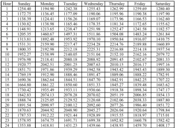
Table 1: Mean value (µ) of load [MW] for each hour of each day of the week for Case 1
Table 2: Standard deviation (σ) of load [MW] for each hour of each day of the week for Case 1
Table 3: Relation between mean and standard deviation (µ/σ) for load for each hour of each day of the week for Case 1
The second database includes daily loadL(k) and daily max-imum temperatureT(k) from the period of January 1, 1997 to January 31, 1999. As the first database, this one was also used in a forecasting competition (Chen et. al., 2004), where the objective was the daily prediction of the load from Jan-uary 1, 1999 to JanJan-uary 31, 1999, i.e., forecasts for 1 to 31 steps ahead. The data from January 1, 1997 to December 31, 1998 was used for input space definition and training of the models. This database can be found at the website http://neuron.tuke.sk/competition. As for case 1, some tics for this database are presented in Table 4. These statis-tics are estimated after detrending the load time-series using a time linear regression model.
the mean value between two registers in the hour (Man-dal et. al., 2005). The objective is to forecast hourly load from one to six hours ahead along the period from September 1, 2003 to September 7, 2003. The data from December 4, 2001 to August 31, 2003 are used for ini-tial input space definition. The same subset selected for training the models in Case 1, i.e., data from the current month, the two previous months and respective pairs from the same period in the last year, are used for development of the models in this case. This database is related to Victoria State and can be found in web at the address at http://www.aemo.com.au/data/aggPD_2000to2005.html. As for case 1, Table 5 to Table 7 presented some statistics for this load time-series, all of them calculated after detrending the load time-series using a time linear regression model.
Table 4: . Mean (µ) [MW], standard deviation (σ) [MW] and
relation between them (µ/σ) of load for each day of the week
for Case 2
µ
! σ
" # µ/σ
Table 5: Mean value (µ) of load [MW] for each day of the
week for Case 2
The hourly and daily load data used in this paper present sea-sonal patterns widely known in load forecasting area namely: hour, week and yearly seasonal pattern (Ferreira and Alves da Silva, 2007), (Hippert et. al., 2001). The yearly pattern is related to the seasons and is modelled by the temperature information. The other patterns are modelled as qualitative information, being represented as binary variables indicating the hour of the day (24 dummies) and day of the week (7 dummies) to be forecasted. The daily database (Case 2) uses only the dummies for day of the week.
Table 8 shows the estimated embedding parametersτ and
d via the first minimum of the mutual information Ix(r)
Table 6: Standard deviation (σ) of load [MW] for each hour of
each day of the week for Case 1
Table 7: Relation between mean (µ) and standard deviation
(σ) for load for each hour of each day of the week for Case 1
and false nearest neighbors method, respectively, and the mean value of the mutual false nearest neighbors statistic
mx(k), y(k). As expected, the value ofmx(k), y(k) confirms that there is synchronism between the reconstructed load and temperature for all cases. The results presented in Table 8 for case 1 confirms that the calculated embedded pa-rameters are invariant characteristics of the attractor, since the values calculated forT(k) andT2(k) are very close.
pre-sented in Table 2 was obtained by highly specialized and dedicated group of modeling experts, while the autonomous models proposed here are mainly automatic, requiring little manual intervention. Further, among the usual parameters that must be specified in neural network training, the ana-lyst must specifies only the maximum dimension parameter
dmax, the confidence levelα(Chaos Input Selection
Algo-rithm) and the maximum number of neurons in the hidden layer to be tested in BIAMLP. Compared with the effort to define heuristically the input space representation, together with the necessity of criteria to neural network structure defi-nition, the autonomous modeling proposed here shows a con-siderable level of automation.
Table 8: Embedding parameters ( (τ, d) and mutual false
nearest neighbors statisticm[·,·]
Case 1 Case 2 Case 3
D τ d τ d τ
L(k) 10 6 12 4 12 13
T(k) 18 13 14 15 19 13
T2(k) 17 13 - - -
-m[l(k), t(k)] 2.96 1.72 1.95
ml(k), t2(k) 2.97 -
-Table 9: MAPE for forecasting period
Case Case Case 3 (steps ahead)
1 2 1 2 3 4 5 6
BIAMLP 4.83 3.25 0.64 1.02 1.55 1.69 1.87 1.88 RVM 8.64 3.00 1.09 1.80 2.10 2.29 2.72 2.94 Benchmark 4.73 1.98 0.56 0.83 1.00 1.15 1.20 1.30
Despite the distinct statistical features of the databases un-der consiun-deration, as presented in Tables 1 to 7, which show significant differences both in level (mean) and variability (standard deviation), the performance of the proposed au-tonomous models, particularly from BIAMLP, was always robust. Even for Case 2, for which BIAMLP presents the worst result when compared with the benchmark, BIAMLP would be ranked in the top five competitors (Chen et. al., 2004). For Case 1 data, BIAMLP’s results are statistically equivalent to the ones obtained by the winner of the compe-tition. Statistical equivalence between the results from BI-AMLP and the corresponding benchmark is also confirmed for Case 3. These findings highlight the robustness of the BI-AMLP’s performance with respect to different time-series.
The importance of qualitative information is demonstrated in Table 10 with the results obtained by BIAMLP when the dummy variables are discarded from the initial input set. In this case, the inputs are all selected from the time-series data, discarding the prior knowledge about the dynamics of the data. The consistent increase on MAPE for the forecasting
period confirms the importance of qualitative information, and shows that Chaos Theory itself does not deal with sea-sonality modeling. Since the calendar information are avail-able for time-series data, the use of this qualitative informa-tion does not reduce the level of automainforma-tion of the proposed models. In fact, qualitative information (general electric load seasonal characteristics) is included based on the premise that calendar information (time, day of the week, and cor-responding month) is available. Therefore, for electric load time series, such qualitative information is automatically in-serted as dummy variables (“1 of n” binary coding). Besides, as the developed neural networks can disregard irrelevant in-formation, such inputs are automatically excluded from the forecasting model when a general seasonal characteristic is not present in a particular dataset.
Table 10: MAPE for forecasting period using Chaos Input Se-lection Algorithm without qualitative information
Case Case Case 3 (steps ahead)
1 2 1 2 3 4 5 6
BIAMLP 11.62 4.37 1.20 1.70 1.88 2.41 2.28 2.66 Benchmark 4.73 1.98 0.56 0.83 1.00 1.15 1.20 1.30
7
CONCLUSION
This work investigates the application of Chaos Theory as a input space representation tool in the development of au-tonomous neural network load forecasting models. Auton-omy should be understood here as a set of automatic and coupled procedures for input space definition and selection, structure specification and complexity control (regulariza-tion). In this work, two neural network-based models are used: the Bayesian Inference Applied to MLPs training and specification (BIAMLPs) and Relevance Vector Machines (RVMs). The obtained results, comparable with the bench-marks available in the literature, specially for the BIAMLPs, show the potential of the proposal. The automation level of the techniques proposed in (Ferreira and Alves da Silva, 2007) has been increased, enabling the application of the new models to problems envolving multiple time series, as for ex-ample, bus load forecasting. Bus load forecasting is needed for feeding important power system control center functions, such as state estimation, generation scheduling, and security assessment.
The result for RVMs, although competitive, can be improved by selecting more appropriate basis functionsΦi(x). One in-teresting theoretical feature of RVMs is the possibility of us-ing different basis functions, such as periodical functions, in order to model seasonal patterns without the use of dummy variables. The development of BIAMLPs considering non-Gaussian noise in the output is another interesting research area, by means of Monte Carlo methods for BIAMLPs defi-nition (Neal, 1996). Beyond those issues, the local modeling of the attractor against the global one used here can still im-prove the results. In order to automate the identification of the regions to be independently modeled, automatic cluster-ing methods are required.
ACKNOWLEDGEMENTS
Special thanks to the support of National Council for Scien-tific and Technological Development (CNPq) that funds the author Alexandre Pinto Alves da Silva and to FAPERJ – Fun-dação Carlos Chagas Filho de Amparo à Pesquisa do Estado do Rio de Janeiro – that funds author Vitor Hugo Ferreira under Grant INST E-26/110.158/2010.
REFERENCES
Abarbanel, H.D.I., Brown, R., Sidorowich, J.J., Tsimring, L.S. (1993) The Analysis of Observed Chaotic Data in Physical Systems,Reviews of Modern Physics, v.65, n.4, pp. 1331-1392.
Amari, S., Murata, N., Müller, K.R., Finke, M., Yang, H. (1996). “Statistical Theory of Overtraining – Is Cross-Validation Asymptotically Effective?”,Advances in Neural Information Processing Systems 8, MIT Press, pp. 176-182.
Bishop, C.M. (1995). Neural Networks for Pattern Recog-nition, Oxford University Press.
Cao, L. (1997). Practical Method for Determining the Min-imum Embedding Dimension of a Scalar Time Series, Physica D, v.110, n.1-2, pp. 43-50.
Cataltepe, Z., Abu-Mostafa, Y.S., Magdon-Ismail, M. (1999). No Free Lunch for Early Stopping”, Neural Computation, v.11, n.4, pp. 995-1009, May 1999.
Chen, B.-J., Chang, M.-W., Lin, C.-J. (2004). Load Fore-casting Using Support Vector Machines: A Study on EUNITE Competition 2001,IEEE Trans. on Power Sys-tems,19(4), pp. 1821-1830.
Ferreira, V.H., Alves da Silva, A.P. (2007). Toward Estimat-ing Autonomous Neural Network-based Electric Load Forecasters, IEEE Transactions on Power Systems,22
(4), n.4, pp. 1554-1562.
Ferreira, V.H., Alves da Silva, A.P. (2009). Automatic Ker-nel Based Models for Short Term Load Forecasting, Proceedings of the 15thInternational Conference on In-telligent System Application to Power Systems, Curitiba, Paraná, Brazil.
Ferreira, V.H., Alves da Silva, A.P. (2010). Teoria do Caos Aplicada à Definição do Conjunto de Entradas de Mod-elos Neurais Autônomos para Previsão de Carga em Curto Prazo. Anais do XVIII Congresso Brasileiro de Automática (XVIII CBA), Bonito-MS, pp.4439-4444.
Fraser, A.M., Swinney, H.L. (1986). Independent Coordi-nates for Strange Attractors from Mutual Information, Physical Review A, v.33, n.2, pp. 1134-1140.
Griffiths, W.E., Hill, R.C., Judge, G.G. (1993). Learning and Practicing Econometrics, John Wiley & Sons.
Guyon, I., Elisseeff, A. (2003). An Introduction to Variable and Feature Selection,Journal of Machine Learning Re-search, n.3, pp. 1157-1182.
Hippert, H.S., Souza, R.C., and Pedreira, C.E. (2001). Neu-ral Networks for Load Forecasting: A Review and Eval-uation,IEEE Transactions on Power Systems, v.16, n.1, pp. 44-55.
Kantz, H., Schreiber, T. (1997). Nonlinear Time Series Analysis, Cambridge Nonlinear Science Series, n.7, Cambridge University Press.
Kennel, M.B., Brown, R., Abarbanel, H.D.I. (1992). De-termining Embedding Dimension for Phase-space Re-construction Using a Geometrical Construction, Physi-cal Review A, v.45, n.6, pp. 3403-3411.
Mackay, D.J.C. (1992). Bayesian Methods for Adaptive Models, Ph.D. dissertation, California Institute of Tech-nology, Pasadena, California, USA.
Mandal, P., Senjyu, T., Uezato, K., Funabashi, T. (2005). Several-Hours-Ahead Electricity Price and Load Fore-casting Using Neural Networks, IEEE PES General Meeting, San Francisco, USA.
Neal, R.M. (1996). Bayesian Learning for Neural Net-works, Lecture Notes in Statistics, n.118, Springer-Verlag, New York.
Ramanathan, R., Engle, R., Granger, C.W.J., Vahid-Araghi, F., Brace, C. (1997). Short-Run Forecasts of Electricity Loads and Peaks,International Journal of Forecasting, v.13, n.2, pp. 161-174.
Schölkopf, B., Smola, A.J., (2002). Learning with Kernels: Support Vector Machines, Regularization, Optimization and Beyond, Cambridge, Massachusetts.
Takens, F. (1981). Detecting Strange Attractors in Turbu-lence, In.: D.A. Rand, L.-S. Young (eds.), Dynamical Systems and Turbulence, Lecture Notes in Mathematics, v.898, pp. 366-381, Springer-Verlag.
Tipping, (2001). Sparse Bayesian Learning and the Rel-evance Vector Machine,Journal of Machine Learning Research, v.1, pp. 211-244.
![Table 4: . Mean ( µ ) [MW], standard deviation ( σ ) [MW] and relation between them (µ/σ ) of load for each day of the week for Case 2](https://thumb-eu.123doks.com/thumbv2/123dok_br/18973740.454627/10.892.457.799.131.374/table-mean-standard-deviation-relation-load-week-case.webp)
