Constructing Minimal Spanning Tree Based on Rough Set Theory for Gene Selection

Soumen Kumar Pati and Asit Kumar Das

Department of Computer Science/Information Technology, St. Thomas‘College of Engineering and Technology, 4, D.H. Road, Kolkata-23

[email protected]

2_{Department of Computer Science and Technology, Bengal Engineering and Science} University, Shibpur, Howrah-03

[email protected]

A

Microarray gene dataset often contains high dimensionalities which cause difficulty in clustering and classification. Datasets containing huge number of genes lead to increased complexity and therefore, degradation of dataset handling performance. Often, all the measured features of these high-dimensional datasets are not relevant for understanding the underlying phenomena of interest. Dimensionality reduction by reduct generation is hence performed as an important step before clustering and classification. The reduced attribute set has the same characteristics as the entire set of attributes in the information system. In this paper, a new attribute reduction technique, based on directed minimal spanning tree and rough set theory is done, for unsupervised learning. The method, firstly, computes a similarity factor between each pair of attributes using indiscernibility relation, a concept of rough set theory. Based on the similarity factors, an attribute similarity set is formed from which a directed weighted graph with vertices as attributes and edge weights as the inverse of the similarity factor is constructed. Then, all possible minimal spanning trees of the graph are generated. From each tree, iteratively, the most important vertex is included in the reduct set and all its out-going edges are removed. The process stops when the edge set is empty, thus producing multiple reducts. The proposed method and some well-known attribute reduction techniques have been applied on several microarray gene datasets for gene selection. The results obtained show the effectiveness of the method.

K

Gene selection, Reduct Generation, Rooted Directed Minimal Spanning Tree, Rough Set Theory, Unsupervised Learning.

1.

I

Feature selection and reduct generation are frequently used as a pre-processing step to data mining and knowledge discovery. It selects an optimal subset of features from the feature space according to a certain evaluation criterion. It has been a fertile field of research and shown very effective in removing irrelevant and redundant features, increasing efficiency in data analysis like clustering, classification, etc. All the measured variables of high-dimensional datasets are not relevant for understanding the underlying phenomena of interest. This enormity in datasets may cause serious problems to many machine learning algorithms with respect to scalability and learning performance. Therefore, feature selection and reduct generation become necessary for data analysis when facing high dimensional data. However, this trend of enormity on both size and dimensionality also poses severe challenges to reduct generation algorithms too. Rough Set Theory (RST) [1, 2], a new mathematical approach to imperfect knowledge, is popularly employed to evaluate significance of attributes and helps to find the reduct.

Hu et al. [3] developed two new algorithms to calculate core attributes and reducts for feature selection. These algorithms can be extensively applied to a wide range of real-life applications with very large data sets. Jensen et al. [4] developed the Quickreduct algorithm to compute a minimal reduct without exhaustively generating all possible subsets and also developed Fuzzy-Rough attribute reduction with application to web categorization. Zhong et al. [5] applies Fuzzy-Rough Sets with Heuristics (RSH) and Rough Sets with Boolean Reasoning (RSBR) for attribute reduction and discretization of real-valued attributes. Komorowski et al. [6] studies an application of rough sets to modeling prognostic power of cardiac tests. Bazan [7] compares rough set-based methods, in particular dynamic reducts, with statistical methods, neural networks, decision trees and decision rules. Carlin et al. [8] presents an application of rough sets for diagnosing suspected acute appendicitis.

The main advantage of rough set theory in data analysis is that it does not need any preliminary or additional information about data like probability in statistics [9], basic probability assignment in Dempster-Shafer theory [10], grade of membership or the value of possibility in fuzzy set theory [11] and so on. But finding reduct by exhaustive search of all possible combinations of attributes is an NP-Complete [12] problem and so some heuristic approach should be applied.

In the paper, a novel reduct generation method is proposed based on indiscernibility relation. Indiscernibility relation induces partitions of objects from which degree of similarity or similarity factor between two attributes is measured and an attribute similarity (AS) set is obtained. Now, the attribute similarities of AS with similarity factor less than that of average are removed and a directed weighted graph is constructed based on the reduced AS set, where attributes are vertices and weight of an edge is the inverse of the similarity factor of corresponding attribute similarity in AS. All possible directed minimal spanning trees are obtained from the directed graph. Each tree represents all important similarities of attributes by its edges which help to find out the information-rich attributes (i.e., vertices) that form the reduct of the data set. For generating a reduct the vertex having maximum degree is selected and included in reduct. Then all its out-going edges are removed. This process continues until the edge set of the tree becomes empty and thus all the selected vertices form a reduct. This is applied to all the trees, multiple reducts are obtained and stored in the set RED.

Finally, the proposed method was applied on several microarray gene datasets for gene selection. Some well-known attribute reduction techniques like PCA [20], SVD [21], etc. were also applied. The reduced datasets were then clustered and the results obtained are compared to show the effectiveness of the method.

experimental resultsand finally conclusion of the paper and the areas for further research are stated in section 5.

2.

R

A

B

Conventionally Before proceeding to explain the proposed method, a review of necessary concepts is done below.

2.1. Indiscernibility Relation

Let Rough set theory is a mathematical technique to deal with incomplete, imprecise or uncertain information. The main idea is based on the indiscernibility relation generated by information about objects of interest that are indistinguishable from each other.

Let I= (U, A) be an information system where U is the finite, non-empty set of objects (called the

universe) and A is a finite, non-empty set of attributes. Each attribute a∈A can be defined mathematically, as a function described in Eq. (1).

: → ∀ ∈ (1)

Where, Va, is the set of values of attribute a, called the domain of a.

For any P ⊆A, there exists a binary relation IND (P), called indiscernibility relation as defined in

Eq. (2).

( ) = ( , ) ∈ ( ) = ( ) ∀ ∈ (2)

Where, fa(x) denotes the value of attribute a for object x in U.

Obviously, IND (P) is an equivalence relation which induces equivalence classes. The family of

all equivalence classes of IND(P), i.e., partition determined by P, is denoted by U/IND(P) or

simply U/P and an equivalence class of U/P, i.e., block of the partition U/P, containing x is denoted by [x]P. If object pair (x, y) belongs to IND (P), x and y are called P-indiscernible.

Equivalence classes IND (P) (or blocks of the partition U/P) are referred to as P-elementary sets.

The indiscernibility relation is used to define the upper and lower approximations in rough set

theory. For each set of attributes P, an indiscernibility relation IND(P) partitions the set of objects

into m number of equivalence classes, defined as partition U/IND(P) or U/P, equal to {[x]p},

where |U/P|=m.

2.2. Reduct and Core Identification

Elements belonging to the same equivalence class are indiscernible; otherwise elements are

discernible with respect to P. If one considers a non-empty attributes subset, R⊂P and IND(R)

=IND (P), then P−R is dispensable. Any minimal R such that IND(R)=IND(P), is a minimal set of

attributes that preserves the indiscernibility relation computed on the set of attributes P and is

called reduct of P, denoted as R=RED(P). Attribute set R is minimal in the sense that [x]R-a [x]P,

∀a ∈R. In other words, no attribute can be removed from set R without changing the equivalence

classes [x]P. The reduct of a decision system is not unique. There may be many subsets of

attributes which are common to all the reducts and are hence, most important to the information

2.3. Algorithm for Rooted Directed Minimal Spanning Tree

Generally, Prim’s [13] or Kruskal’s [14] algorithm is used to find the minimal spanning tree (MST) of an undirected graph. But they do not give the optimal result when applied to directed graphs. Fig. 1 exhibits that the tree, constructed by taking iterative greedy decision of Prim’s algorithm, is not a minimal spanning tree of the directed graph.

Chu and Liu [15], Edmonds [16] and Bock [17] have independently given efficient algorithms for finding the MST on a directed graph. The Chu-Liu and Edmonds algorithms are virtually identical; the Bock algorithm is similar but stated on matrices instead of on graphs. Furthermore, a distributed algorithm is given by Humblet [18].

Figure 1. MST construction for directed graph using Prim’s algorithm

The rooted directed spanning tree is defined as a graph which connects, without any cycle, all

vertices with n-1 edges, i.e., each vertex, except the root, has one and only one incoming edge.

Consider a directed graph, G=(V, E), where V and E are the set of vertices and edges,

respectively. A cost c(i, j) is associated with each edge (i, j) in E. Let |V|=n and |E|=m. The algorithm is described and explained briefly by the following steps, which computes a rooted

directed minimal spanning tree MST(V, S) of the graph G(V, E) where S is a subset of E such that

c(i, j),∀(i , j) in S is minimized.

Chu-Liu/Edmond’s (CLE) Algorithm

1. Discard the edges entering the root if any; for each vertex other than the root,

select the entering edge with the smallest cost. Let the selected n-1 edges be the

set S.

2. If no cycle formed, MST (V, S) is a MST. Otherwise, go to step 3.

3. For each cycle formed, contract the vertex in the cycle into a pseudo-vertex(k)

and modify the cost of each edge which enters a vertex(j) in the cycle from some

vertex(i) outside the cycle, according to the Eq. (3).

( , ) = ( , !) − ( ( (!), !) − min&(c(x(j), j) (3)

Where c(x(j),j) is the cost of the edge in the cycle which enters j.

4. For each pseudo-vertex, select the entering edge which has the smallest modified

cost; replace the edge which enters the same real vertex in S by the new selected

edge.

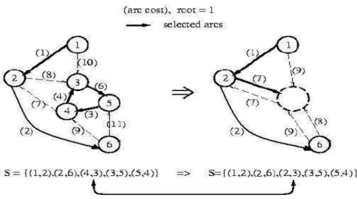
The key idea of the algorithm is to find the replacing edge(s) which has the minimum extra cost to eliminate cycle(s), if any. The Eq. (3) exhibits the associated extra cost. Figure 2. illustrates that the contraction technique finds the minimum extra cost replacing edge (2, 3) for edge (4, 3) and hence the cycle is eliminated.

3.

M

R

G

M

The proposed method first computes the equivalence classes by IND(Ai) for each attribute Ai.

Then, it calculates the degree of similarity among each pair of attributes with the help of a similarity factor. Based on the similarity of attribute pairs a weighted directed graph is formed and all possible minimal spanning trees of the graph are obtained which finally generate the multiple reducts for gene selection.

Figure 2. MST construction using Chu-Liu / Edmond’s algorithm

To illustrate the method, a sample dataset, shown in Table 1, with eight objects and four attributes is considered.

Table1. Sample dataset

Object Diploma(i) Experience (e) French (f) Reference(r)

x1 MBA Medium Yes Excellent

x2 MBA Low Yes Neutral

x3 MCE Low Yes Good

x4 MSc High Yes Neutral

x5 MSc Medium Yes Neutral

x6 MSc High Yes Excellent

x7 MBA High No Good

x8 MCE Low No Excellent

U/i = ({x1, x2, x7}, {x3, x8}, {x4, x5, x6}) U/e = ({x1, x5}, {x2, x3, x8}, {x4, x6, x7}) U/f = ({x1, x2, x3, x4, x5, x6}, {x7, x8}) U/r = ({x1, x6, x8}, {x2, x4, x5}, {x3, x7})

3.1. Attribute Similarity Measurement

Elements An attribute Ai is similar to another attribute Aj in context of indiscernibility if they

induce the same equivalence classes of objects under their respective indiscernibility relations. But in real situation, it rarely occurs. So similarity of attributes is measured by introducing a similarity factor, based on indiscernibility relation, which indicates the degree of similarity of one attribute to another attribute. Here, an attribute Ai is said to be similar to an attribute Aj with

degree of similarity (or similarity factor) ₊,,-and is denoted by _, .

/,0

12 - if the probability of

inducing the same equivalence classes of objects under their respective indiscernibility relations

is ( ₊,,-×100)%, where ₊,,-is computed by Eq. (4).

34,,-= 1

5 6 5_, 7

1

|[ ]:/|

[;]_{</=> :}6 _/

? _{[;]<0∈> :}

0

6 @[ ]:/∩ [ ]:0B (4)

It is quite obvious that ₊,,- would have value 1 if Ai and Aj have exactly similar classification

pattern. For each pair of conditional attributes (Ai, Aj), similarity factor is computed by Eq. (4).

The method of computation of similarity measurement for the attribute similarity _, .

/,0

12 - (Ai Aj)

is described in algorithm “SIM_FAC” below.

Algorithm: SIM_FAC(Ai, Aj)

/* Similarity factor computation for Ai→_{Aj */}

Input: Attributes Ai and Aj

Output: Similarity factor ₊ ,,-Begin

Compute indiscernibility IND(Ai) using Eq. (2)

Compute indiscernibility IND(Aj) using Eq. (2)

/* similarity measurement of Ai to Aj */

3₄,,-= 0

For each [ ]_:/ ∈ E _,{

max_overlap = 0 For each [ ]_:0 ∈ E _-{

Overlap = |[ ]_:/∩ [ ]_:0| If (overlap > max_overlap) then max_overlap = overlap }

₄,,-= ₄,,-+ GHI _KLMNO P

| [;]_</ |

₄,,-= . /,0

|> :E |/ End.

3.2. Formation of Attribute Similarity Set

For each pair of conditional attributes (Ai, Aj), similarity factor is computed by “SIM_FAC”

algorithm, described in the previous sub-section. High value of similarity factor of Ai→_{Aj means}

that the indiscernibility relations IND(Ai) and IND(Aj) produce highly similar equivalence classes.

This implies that both the attributes Ai and Aj have almost similar classification power and so

Ai→_{Aj is considered as strong similarity of Ai to Aj. Since, for any two attributes Ai and Aj, two}

similarities Ai→_{Aj and Aj}→_{Ai are obtained, only the one with higher similarity factor is included}

in the attribute similarity set AS. In case, both have equal values of similarity factors, any one is

chosen randomly. Thus, for n attributes, Q(QRS) similarities are selected, of which some are strong

and some are not. Out of these, the similarities with ₊,,- value less than the average value δ_{f of all}

the similarity factors, are discarded and the rest are considered as the set of attribute similarity AS.

So, each element x in AS is of the form x: Ai→_{Aj such that Left(x)=Ai and Right(x)=Aj. The}

algorithm “AS_GEN” described below, computes the attribute similarity set AS.

Algorithm: AS_GEN (A, δδδδ_f)

/* Computes attribute similarity set {Ai→Aj} */

Input: A = set of attributes and δf = 2-D matrix containing similarity factors between each pair of conditional attributes, obtained using Eq. (4).

Output: Attribute Similarity Set AS Begin

AS = {}, sum_δ_{f = 0}

/* add n(n – 1)/2 elements to AS */ For i = 1 to (|C| - 1) {

For j = i+1 to |C| {

If ( ₄,,-> ₄-,,) {

sum_δ_{f = sum_}δ_{f + 4} AS = AS ∪ {Ai→Aj} }

Else {

sum_δ_{f = sum_}δ_{f + 4}-,, AS = AS ∪ {Aj→ Ai} }

} }

/*modify AS to store only {Ai→_{Aj}for which 4},,- > _{avg_}δ_{f */}

avg_δ_f = UVG_ +

|W|(|W|RS)

For each {Ai→Aj}∈AS

AS = AS – {Ai→Aj} End.

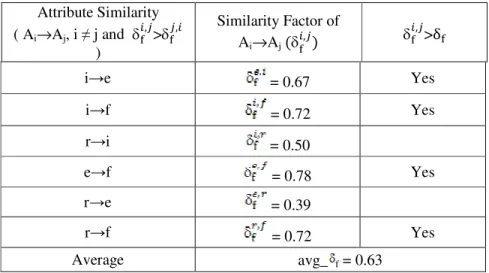
Initially, algorithm “AS_GEN” selects AS= {i e, i f, r i, e f, r e, r f} and constructs

Table 2. As the similarity factors for attribute similarities i e, i f, e f and r f are greater than

the average similarity factor avg_δ_{f = 0.63, modified attribute similarity set AS= {i} e, i f, e f,

r f }.

Table 2. Selection of attribute similarities in AS

Attribute Similarity ( Ai→_{Aj, i j and +},,-_{> +}-,,

)

Similarity Factor of Ai→_Aj (

+

,,-_{) +},,->δ₊

i e _{= 0.67} Yes

i f _{= 0.72} Yes

r i _{= 0.50}

e f _{= 0.78} Yes

r e _{= 0.39}

r f _{= 0.72} Yes

Average avg_ f = 0.63

3.3. Construction of Attribute Similarity Graph

The minimized attribute similarity set AS= { _, .

/,0

12 -} contains the set of pairs of attributes that

are most strongly related to each other. To generate a reduct, firstly this set is represented by a

directed graph, called attribute similarity graph (ASG). The vertices of ASG are the attributes

present in the set AS and weighted edge exists from attribute Ai to attribute Aj with weight +,,- if

, .

/,0

12 -∈AS. The weight of an edge between two vertices is the value of the similarity factor

between those two attributes of the data set. Thus, attribute similarity Ai→_{Aj with +},,-_{=w, present}

in set AS is represented by a directed edge from vertex Ai to vertex Aj with weight w.

Mathematically, ASG is denoted as G(V, E) where

= Z ,[ , ∈ \]^ _( ) ∪ a bℎ_( )d∀ ∈ ef (5)

h = i\ ,, -dj , k_./,0

12 - ∈ el (6)

Figure 3. ASG obtained from Table 2.

3.3. Directed Minimal Spanning Tree(s) Construction

The ASG, therefore, represents the total similarity structure of the attribute similarity set AS.

Some vertices in the ASG may have multiple incoming edges which imply that a particular vertex

(attribute) v is similar to more than one other vertex (attribute). Now, the vertices of the graph,

which have one or more out-going edges, represent the attributes to which some other attributes are similar. The weights of the edges between them denote the strength of their similarity. Therefore, a maximal spanning tree of this graph would give the highest similarities between two attributes. Constructing maximal spanning tree is equivalent to constructing minimal spanning tree with the weights inversed. So, to construct the minimal spanning tree, weights associated to each edge of the directed graph ASG are inversed and Chu-Liu / Edmond’s Algorithm is applied.

For instance, edge weight w is replaced by w-1. In the process, the vertex that has only outgoing

edges and no incoming edges is considered as the root. If more than one such vertex exists, then they are fused to form a single vertex. So, before construction of the minimal spanning tree, ASG is modified to merge all the nodes with in-degree zero to a single node and it is considered as the

root of the graph. That means the new node A’ formed by merging other nodes is given by Eq.

(7).

n_{= o} , ,

, p^bR₍

,) = 0 (7)

where, deg - (Ai) denotes in-degree of vertex A’, A’ becomes the tail of all outgoing edges from

each Ai and heads of the outgoing edges from each Ai remain the same. Thus, A’ is the root of the

graph as it does not have any incoming edge.

Now, a graph can have multiple minimal spanning trees. This happens when more than one edge, entering the same node, have minimum weights. Keeping track of such edges and using Chu-Liu / Edmond’s Algorithm, all possible directed minimal spanning trees of the graph are generated.

Algorithm: MST_GEN (AS)

/* generates minimal spanning trees of ASG */

Input: AS = attribute similarity set obtained from AS_GEN algorithm.

Output: Set of Rooted Directed Minimal Spanning Trees M Begin

/* Represent AS as a graph using Eq. (5) and Eq. (6) */ Construct graph ASG = (V, E) where

V = {Ai | Ai ∈ (Left(x) ∪ _Right(x)),∀_x ∈ _AS}

E = {(Ai, Aj)| _, .

/,0

12 -∈ AS }

For each node Ni ∈ V If (deg-(Ni) = 0) then {

Root = Root ∪ _{Ni}

Modify ASG by fusing all vertices in set Root }

For each edge _, .

/,0

12 -∈ E ₊,,-= ( ₊,,-)-1

Compute set of all possible Directed Minimal Spanning Trees M of the ASG using CLE_algorithm

End.

The algorithm modifies the attribute similarity graph shown in Fig. 3 to a new graph, as shown in Fig. 4 and constructs all possible directed minimal spanning tree(s), shown in Fig. 5 (in this case only one such tree is possible).

Figure 4. Modified ASG obtained from Figure 3.

Figure 5. Minimal spanning tree(s) of the graph in Figure 4.

3.5. Multiple Reducts Generation

The above generated rooted directed minimal spanning tree would give the highest similarities between pairs of attributes. Now, our aim is to reduce the number of attributes but also preserve the equivalence class structure of the dataset considering all the attributes. To do this, the attributes, which produce equivalence classes similar to that of some other attribute, may be neglected without affecting the overall equivalence class structure of the dataset. Therefore, on the basis of attribute similarity, those attributes to which some other attributes are similar, are the most important ones and hence should be considered as the reduct.

Now, the tail of every edge ei∈E of a directed minimal spanning tree mj=(Vj, Sj), ∀mj∈M denotes

an attribute to which some other attribute is similar. So, every attribute Tail(ei), ∀ei∈E should be

The minimal spanning tree is searched to find the vertex with highest out-degree. The vertex with highest out-degree is an attribute to which most number of other attributes are similar. So, this

node is added to the initially empty reduct set Rj and its out-going edges are removed from the

tree. This process of trimming the edges of the tree and adding the vertex (attribute) to the reduct

set continues till the edge set of the tree becomes empty and thus final reduct Rj is obtained.

Basically, it performs vertex covering of the tree.

Repeating this process for all the generated directed minimal spanning trees, multiple reducts Rj

are obtained and the set RED of all Rj gives the multiple reducts for the dataset.

Algorithm: RED_GEN (M)

/*generates multiple reducts from all possible rooted directed minimal spanning trees M of ASG */

Input: M = Set of All Possible Rooted Directed Minimal Spanning Trees Output: RED = Set of Multiple Reducts

Begin

RED = { } For j = 1 to |M| { Rj = { }

Order [Vj] = array of vertices of minimal spanning tree mj∈M sorted in descending order of their out-degree

For i = 1 to | Vj | {

Remove outgoing edges in mj from vertex order[i] Rj = Rj∪ {order[i]}

If (Sj = ) then

RED = RED ∪ _{Rj}

} }

Return (RED) End.

Reduct generated from Fig. 5 is {i, r, e} as shown in Figure 6.

4.

The proposed method computes multiple reducts (gene selection) for different kinds of microarray gene datasets (cancerous data), few of which are summarized below:

• Leukemia (ALL v.s. AML) dataset: Training dataset consists of 38 bone marrow samples (27 ALL and 11 AML), over 7129 human genes. The raw data is available at http://www-genome.wi.mit.edu/cgi bin/cancer/datasets. cgi.

• _{Lung Cancer dataset: Training dataset contains 16 samples labeled as "MPM" and 16} samples labeled as "ADCA" with around 12533 genes. The raw data available at http://www.chestsurg.org/microarray.htm.

• Prostate Cancer dataset: Training dataset contains 52 samples labeled as "relapse" and 50 patients having remained relapse free labeled as "non-relapse" prostate samples with

around 12600 genes. The raw data available at

http://www-genome.wi.mit.edu/mpr/prostate.

• _{Colon Cancer dataset: The colon cancer data contains 62 samples collected from} colon-cancer patients. Among them, 40 tumor biopsies are from tumors (labeled as "negative") and 22 normal (labeled as "positive") biopsies are from healthy parts of the colons of the same patients. 2000 out of around 6500 genes were selected based on the confidence in

the measured expression levels. The raw data available at

http://microarray.princeton.edu/oncology/ affydata/index.html.

• _{Central Nervous System dataset: Patients’ outcome prediction for central}

nervous system embryonic tumor. Survivors are patients who are alive after treatment whiles the failures are those who succumbed to their disease. The data set contains 60 patient samples, 21 are survivors (labeled as "Class1") and 39 are failures (labeled as "Class0"). There are 7129 genes in the dataset. The raw data available at http://www-genome.wi.mit.edu/mpr/CNS.

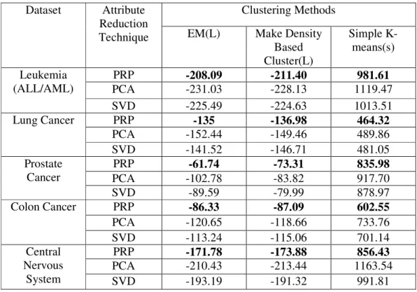
At first, all the numeric attributes are discretized by ChiMerge [19] discretization algorithm. The proposed method (PRP) and some well-known dimensionality reduction methods for unsupervised learning such as, Principle Component Analysis (PCA) [20] and Singular Value

Decomposition (SVD) [21] were applied on the datasets. The reduced datasets were then

Table 3. Comparison of Proposed, PCA and SVD methods

Dataset Attribute Reduction Technique

Clustering Methods

EM(L) Make Density Based Cluster(L)

Simple K-means(s)

Leukemia (ALL/AML)

PRP -208.09 -211.40 981.61

PCA -231.03 -228.13 1119.47

SVD -225.49 -224.63 1013.51

Lung Cancer PRP -135 -136.98 464.32

PCA -152.44 -149.46 489.86

SVD -141.52 -146.71 481.05

Prostate Cancer

PRP -61.74 -73.31 835.98

PCA -102.78 -83.82 917.70

SVD -89.59 -79.99 878.97

Colon Cancer PRP -86.33 -87.09 602.55

PCA -120.65 -118.66 733.76

SVD -113.24 -115.06 701.14

Central Nervous

System

PRP -171.78 -173.88 856.43

PCA -210.43 -213.44 1163.54

SVD -193.19 -191.32 991.81

5.

D

C

Systematic and unbiased approach to cancer classification is of great importance to cancer treatment and drug discovery. It has been known that gene expression contains the keys to the fundamental problems of cancer diagnosis, cancer treatment and drug discovery. The recent advent of microarray technology has made the production of large amount of gene expression data possible. This has motivated the researchers in proposing different cancer classification algorithms using gene expression data.

This paper describes a new method of attribute reduction using concepts of Rough Set Theory and Graph Theory. In this method multiple reducts are generated. Here, the data mining problem is converted to graph theoretic problem and then solved. Many attribute reduction techniques use heuristic algorithms which often degrade the performance. But this method has a strong mathematical background and hence, produces good results. This method of attribute reduction is applied on microarray gene dataset to select a subset of important genes. Future enhancements to this work may include integration of the multiple reducts generated to form a better quality single reduct using some techniques.

R

[1] Pawlak, Z., (1982) “Rough sets”, International journal of information and computer sciences.,Vol. 11, pp. 341-356.

[2] Pawlak, Z., (1998) “Rough set theory and its applications to data analysis”, Cybernetics and systems,

vol. 29, pp. 661-688.

[3] Hu, X., Lin, T.Y. & Jianchao, J., (2004) “A New Rough Sets Model Based on Database Systems”,

[4] Jensen R. & QiangShen, (2004) “Fuzzy-Rough Attribute Reduction with Application to Web Categorization”, Fuzzy Sets and Systems, Vol.141, No.3, pp.469-485.

[5] Zhong, N. & Skowron, A., (2005) “A Rough Set-Based Knowledge Discovery Process”, International Journal of Applied Mathematics and Computer Science. Vol. 11(3), pp. 603-619.

[6] Komorowski, J. & Ohrn, A., (1999) “Modelling Prognostic Power of Cardiac tests using rough sets”,

Artificial Intelligence in Medicine, vol. 15, pp. 167-191.

[7] Bazan, J., (1998)“A Comparison of dynamic and nondynamic rough set methods for extracting laws from decision tables”, Rough Sets in Knowledge Discovery, PhysicaVerlag.

[8] Carlin, U., Komorowski, J. & Ohrn, A., (1998) “Rough Set Analysis of Patients with Suspected Acute Appendicitis”, Proceeding IPMU.

[9] Devroye, L., Gyorfi, L., & Lugosi, G., (1996) “A Probabilistic Theory of Pattern Recognition”, Newyork: Springer-Verlag.

[10] Gupta, S. C. & Kapoor, V. K., (1994) “Fundamental of Mathematical Statistics”, Published by: Sultan Chand & Sons, A.S. Printing Press, India.

[11] Pal, S., K., & Mitra, S., (1999) “Neuro-Fuzzy pattern Recognition: Methods in Soft Computing”, New York: Willey.

[12] Garey, M. & Johnson, D., (1979) “Computers and intractability - A guide to the theory of NP-completeness”, Freeman, New York.

[13] Prim, R. C., (1957) “Shortest connection networks and some generalizations”, In: Bell System Technical Journal, pp. 1389-1401.

[14] Joseph, Kruskal, B., (1956) “On the shortest Spanning Subtree of a graph and the traveling salesman problem”, In: Proceedings of the American Mathematical Society, Vol. 7, pp. 48-50.

[15] Chu, Y. J. & Liu, T. H., (1965) “On the shortest arborescence of a directed graph”, Science Sinica, vol.14, pp.1396-1400.

[16] Edmonds, J., (1967) “Optimum branching”, J. Research of the National Bureau of Standards, 71B, pp.233-240.

[17] Bock, F., (1971) “An algorithm to construct a minimum spanning tree in a directed network”,

Developments in Operations Research, Gordon and Breach, NY, pp. 29-44.

[18] Humblet, P., (1983) “A distributed algorithm for minimum weighted directed spanning trees”, IEEE Trans. on Communications, vol. COM-31, no.6, pp.756-762.

[19] Kerber, R. & ChiMerge, (1992) “Discretization of Numeric Attributes”, in Proceedings of AAAI-92,

Ninth International Conf. Artificial Intelligence, AAAI-Press, pp. 123-128.

[20] Mozer, M. C., Jordan, M. I. & Petsche T., (1997) “A principled alternative to the self-organising map”, in Advances in Neural Information Processing Systems, vol. 9, MIT Press, Cambridge, MA. [21] Petrou M. & Bosdogianni, P., (2000) “Image Processing: The Fundamentals-an example of SVD”,

John Wiley, pp. 37-44.

Authors

Mr. Soumen Kumar Pati is an Assistant Professor of Computer Science/Information Technology at St. Thomas’ College of Engineering and Technology, Kidderpore, Kolkata,West Bengal, India. He has received M.Tech degree in Computer Science and Engg from Jadavpur University. He is registered for PhD (Engg) degree at Bengal Engineering and Science University, Shibpur, Howrah. His research interests include Bio-informatics, Data Mining and Pattern Recognition, Roughset Theory, etc.