Detection of Denial of Service Attack in Wireless
Network using Dominance based Rough Set
N.
Syed
Siraj
Ahmed
SchoolofComputing scienceandEngineering VITUniversity
Vellore,India632014
D.
P.
Acharjya
Schoolof ComputingscienceandEngineering VITUniversity
Vellore,India632014
Abstract—Denial-of-service (DoS) attack is aim to block the services of victim system either temporarily or permanently by sending huge amount of garbage traffic data in various types of protocols such as transmission control protocol, user datagram protocol, internet connecting message protocol, and hypertext transfer protocol using single or multiple attacker nodes. Maintenance of uninterrupted service system is technically difficult as well as economically costly. With the invention of new vulnerabilities to system new techniques for determining these vulnerabilities have been implemented. In general, probabilistic packet marking (PPM) and deterministic packet marking (DPM) is used to identify DoS attacks. Later, intelligent decision proto-type was proposed. The main advantage is that it can be used with both PPM and DPM. But it is observed that, data available in the wireless network information system contains uncertainties. Therefore, an effort has been made to detect DoS attack using dominance based rough set. The accuracy of the proposed model obtained over the KDD cup dataset is 99.76 and it is higher than the accuracy achieved by resilient back propagation (RBP) model.
Keywords—Denial of service; Rough set; Lower and upper approximation; Dominance relation; Data analysis
I. INTRODUCTION
Denial-of-service attack is one of the most threatening security issues in wireless networks. Over the past few years, it is observed that while surfing websites on the internet a computer in the network host may have been the target of denial-of-service attacks using various protocols such as TCP, UDP, ICMP, and HTTP. Among which TCP flooding is the most prevalent [1]. This results in disruption of services at high cost. The main objective of denial-of-service attack is to consume a large amount of resources, thus preventing legitimate users from receiving service with some minimum performance. TCP flooding [1] exploits TCPs three-way hand-shake procedure, and specifically its limitation in maintaining half-open connections. Denial of service attack is a technique to make a host or network resource block to its intended users. The attack temporarily or permanently interrupts or suspends services of a computer in the network host connected to the Internet. A permanent denial-of-service attack damages a system so badly that it requires replacement or reinstallation of hardware such as routers, printers, or other network hardware. Hence in general, detection is required before the spread of this attack. Detection of such an attack is often a part of information security [2, 3]. Therefore, it is essential to secure wireless networks from such an attack.
A distributed denial of service (DDoS) attack is a simul-taneous network attack on a victim from a large number of compromised hosts, which may be distributed widely among different, independent networks [4]. By exploiting asymmetry between network wide resources, and local capacities of a victim a DDoS attack can build up an intended congestion very quickly. The Internet routing infrastructure, which is stateless and based mainly on destination addresses, appears extremely vulnerable to such coordinated attacks. It is a type of cyber attacks in which the victim will be overloaded and will not able to perform any normal functions. Many researchers have presented their work in various directions. Gavrilis and Dermatas uses radial basis function neural network and sta-tistical features to achieve accurate classification of abnormal activity under DDoS attack without interfering normal traffic [5]. The advantage of this method is that it can block the traffic selectively based on the attack. Wang et al. introduced a queuing model for the evaluation of the denial of service attacks in computer networks. The network is characterized by a two-dimensional embedded Markov chain model. It helps in developing a memory-efficient algorithm for finding the stationary probability distribution which can be used to find other interesting performance metrics such as connection loss probability and buffer occupancy percentages of half-open connections [6]. Gelenbe and Lukes proposed a model to defense denial of service attack using cognitive packet network infrastructure. The technique uses smart packets to select paths based on quality of service [7].
Mell introduces resistant intrusion detection system archi-tecture to counter denial of service attack. The components of intrusion detection system architecture are invisible to the attacker and also this architecture relocates intrusion detection system components from attacked hosts. This is achieved by using mobile agent technology [8]. Hamdi uses outbound and inbound demilitarized zone to detect denial of service attack. The major advantage is that it also identifies synchronize-flooding attack [9]. Later, Chen et al., applied targeted filtering method to identify a distributed denial of service attack. The advantage is that it can be deployed at a local firewall. But, it takes extra time to detect the attack [10]. Rajkumar and Selvakumar proposed a model using Resilient back propaga-tion (RBP) algorithm as the base classifier for the detecpropaga-tion of denial of service attack [11]. From the literature survey, it is understood that much research is carried out for the detection of denial of service attack and distributed denial of service attack.
Denial-of-service attacks commonly block the services of legitimate user in a wireless network either temporarily oe per-manently by supplying either short term orlong term harmful artificial traffic. Additionally, it is observed that the informa-tion system pertaining to denial-of-service attack in wireless network contains uncertainties and the attributes involved in the information system have some specific order. To deal with such uncertainties, criteria, and specific order the concept of dominance based rough set can be used. This motivation help us to think a alternative approach using dominance based rough set.
In this paper, we propose an alternative method using dominance based rough set for the detection of denial of service attack. The rest of the paper is organized as follows: we discuss basic concepts of dominance based rough set in section 2. Section 3 discusses dominance principle. A case study is presented in section 4 to analyze and track denial of service attack using dominance based rough set. Finally, the paper is concluded with a conclusion.
II. FOUNDATION OFINFORMATIONSYSTEM
An information system provides an expedient to describe a finite set of objects called the universe with a finite set of attributes thereby represents all the available information and knowledge. Formally, it is defined as a four tuple T = (U, A, V, f)whereU ={x1, x2,· · ·, xn}is a non-empty finite
set of objects called the universe, A ={a1, a2,· · ·, an} is a
nonempty finite set attributes. The component V is defined as V =∪a∈AVa, where Va is the set of attribute values that
an attribute a may take. The component f : (U ×A) → V is an information function. The information system is said to be a decision system if A=C∪ {d}, C 6=φ,{d} 6=φ and C∩ {d}=φ whereC is a set of conditional attributes and d is the decision [12].
Let B ⊆ A. Two objects xi and xj are said to be
B-indiscrinble if f(xi, a) =f(xj, a) for all a∈B.
Mathemat-ically, we denote it as IN D(B) is defined as below and we writexiIBxj.
IN D(B) =
(xi, xj)∈U2:f(xi, a) =f(xj, a)∀a∈B
Object xj dominates object xi on criteria a if Vaxj ≤ Vaxi,
whereVxj
a is the attribute value of objectxj on criteriaa. Let
Q ⊆C be a criteria set. Let us define a dominance relation dm(Q)onU as
dm(Q) =
(xi, xj)∈U2:Vaxj ≤Vaxi∀a∈Q (1)
If (xi, xj)∈dm(Q), then we writexjDQxi. LetP ⊆C is a
criteria set. Let us define D+P(xi),P-dominatingxi as below.
D+
P(xi) ={xj∈U :xjDPxi} (2)
Similarly, we define a setD−P(xi),P-dominated byxias below.
D−
P(xi) ={xj∈U :xiDPxj} (3)
Two object xi and xj are said to be inconsistent, if their
criterion do not satisfy dominance principle with ordered decision class [13].
III. DOMINANCE BASEDROUGHSET
Rough set of Pawlak is a mathematical tool used in data analysis in particular to analyze uncertainties [14]. But it fails to analyze data containing preference order and may lead to loss of information. To overcome the limitations the concept of dominance based rough set is introduced [15, 16, 17]. In dominance based rough set, given a set of objects, there is a criterion at least among condition attributes. Additionally attributes like color, country may not be of preference ordered. Therefore, criteria attributes are divided into ordered decision classes based on decision attribute. Also criteria in condition attributes are correlated semantically with ordered decision attribute by means of dominance relation.
Formally, dominance based rough set (DRS) is based on the concept of dominance principle to extract knowledge from the information system. Here, the classification is carried out based on decision class(d). Therefore, the decision(d)divides the universeU into finite number of classes, CL, such as
CL={CLi:i∈T};T ={1,2,3,· · ·, m}
Additionally, these classes are ordered. It means that, if r, s∈ T andr > s, then the objects of classClr are preferred then
the objects of classCls. The upward and downward unions of
every elementCliofCLis given asCli≥andCl
≤
i respectively.
Mathematically, it is defined as
Cl≥i =∪j≥iClj;Cl≤i =∪j≤iClj
LetQ⊆C, objects certainly belongs toCli≥ andCl≤i are in their lower approximations Q(Cli≥) and Q(Cli≤) respec-tively. The lower approximations are defined as below.
Q(Cli≥) =nx∈U :D+
Q⊆Cl
≥
i
o
(4)
Q(Cli≤) =nx∈U :D−Q⊆Cli≤o (5)
Similarly, objects possibly belong toCli≥ andCli≤ are in their upper approximationsQ(Cl≥i )andQ(Cli≤)respectively. It is defined as below.
Q(Cli≥) = [
x∈Cl≥i
D+
Q(x) (6)
Q(Cli≤) = [
x∈Cl≤i
D−
Q(x) (7)
The boundary region of Cli≥ and Cl
≥
i , which contains
am-biguous elements are defined as below
BNQ(Cli≥) =Q(Cl
≥
i )−Q(Cl
≥
i )
BNQ(Cli≤) =Q(Cl
≤
i )−Q(Cl
≤
i )
A. Dominance Relation Based Rule Formation
For a given information system, the dominance principle is capable of deducing more generalized description of objects. This can be done by means of upward and downward union of rough approximation. This is a fundamental concept in a knowledge discovery.
LetQ⊆C be a conditional attributes. Based on the rough approximation, the Q-lower and Q-upper approximations are computed on criterion attribute to extract the knowledge. The rules generated from criterion attribute using upward and downward union of Q-lower, Q-upper approximations are of the form “If Condition then Decision”.
In real life situation, the data collected may be uncertain, vague and imprecise which may leads to inconsistency. The inconsistency data are identified in rough set by means of indiscernible relation. Likewise the inconsistency presents in the collected data are identified in dominance based rough set on employing dominance relation. The two objects are said to be inconsistent when the criteria attributes do not satisfy dominance principle with decision attribute. Further such inconsistency exists in logic must be removed try as it leads to error decision. The simplest way to remove such inconsistency is to omit the inconsistent objects. The five kinds of determinate rules associated with dominance based rough set are defined as follows [13].
1) For all criteria ai ∈ Q ⊆ C; if f(x, a1) ≥ Vax1
and f(x, a2) ≥ Vax2 and · · · f(x, ai) ≥ V
x ai, then x∈Cl≥t wheret∈ {2,3,· · · , n}. Rules generated in
such way called as certain D≥ decision rules. These rules are obtained fromQ(Cl≥t).
2) For all criteria ai ∈ Q ⊆ C; if f(x, a1) ≥ Vax1
and f(x, a2) ≥ Vax2 and · · · f(x, ai) ≥ Vaxi, then x ∈Cl≥t where t ∈ {2,3,· · ·, n}. Rules generated in such way called as possible D≥ decision rules. These rules are obtained from Q(Cl≥t).
3) For all criteria ai ∈ Q ⊆ C; if f(x, a1) ≤ Vax1
and f(x, a2) ≤ Vax2 and · · · f(x, ai) ≤ Vaxi, then x ∈ Clt≤ where t ∈ {1,2,· · · ,(n−1)}. Rules
generated in such way called as certainD≤ decision rules. These rules are obtained from Q(Cl≤t).
4) For all criteria ai ∈Q ⊆C; if f(x, a1)≤Vax1 and
f(x, a2) ≤ Vax2 and · · · f(x, ai) ≤ Vaxi, then x ∈ Clt≤ wheret∈ {1,2,· · · ,(n−1)}. Rules generated
in such way called as possible D≤ decision rules. These rules are obtained from Q(Cl≤t).
5) Let O1 = {a1, a2,· · ·, ak} ⊆ C; O2 = {ak+1,
ak+2,· · ·, ai} ⊆ C; Q = (O1 ∪ O2); O1 and
O2 are not necessarily disjoint. If f(x, a1) ≥ Vax1
and f(x, a2) ≥ Vax2, · · ·, and f(x, ak) ≥ Vaxk and f(x, ak+1) ≤ Vaxk+1 and f(x, ak+2) ≤ Vaxk+2, · · ·
andf(x, ai)≤Vaxi, thenx∈Clu∪Clu+1∪· · ·∪Clv, where r ≤ u ≤ v ≤ t and r, u, v, t ∈ T. Rules generated in such way called as approximate D≥≤ decision rules. These rules are obtained from Q(Cl≤
r)∩Q(Cl
≥
t).
The rules 1 and 3 represent certain knowledge whereas rules 2 and 4 represent possible knowledge that can be
ex-tracted from the information system. The rules 5 represent am-biguous knowledge. Ify∈Q(Cl≥t)such that f(y, a1) =Vay1,
f(y, a2) =Vay2,· · ·,f(y, ai) =Vayi, thenyis called as basis of the rule. An object which matches both condition and decision parts of a rule supports the decision rule. An object which meets only condition part of a rule is covered by a decision rule. Decision rules either certain or approximate is said to be complete if it satisfies following conditions.
1) Each x∈Q(Cl≥t) must support at least one certain D≥ decision rule whose consequent is x ∈ Cl≥
r
wherer, t∈ {2,3,· · · , n} andr≥t.
2) Each x∈Q(Cl≤t) must support at least one certain
D≤ decision rule whose consequent is x ∈ Cl≤
r
wherer, t∈ {1,2,· · · ,(n−1)}andr≤t. 3) Each x ∈ (Q(Cl≤
r) ∩ Q(Cl
≥
t)) must support at
least one approximate D≥≤ decision rule whose consequent is x ∈ Clu∪Clu+1∪ · · · ∪Clv where
r≤u≤v≤t andr, u, v, t∈T.
It means that, the set of rules must cover all objects of the information system. Additionally, it assigns consistent objects to their original classes and inconsistent objects to clusters of classes pertaining to this inconsistency.
IV. PROPOSEDRESEARCHDESIGN
A common type of attack used to block the service of the wireless network in recent years is denial of service attack. Therefore, recognizing such an attack is of great challenge. To this end, in this section, we purpose our research design for detecting dos attack. The following Figure 1 depicts an abstract view of the model. The initial step of any model development is problem identification that includes basic knowledge of the problem undertaken. The data collected initially preprocessed. The main objective is to transform the raw input data into an appropriate format for subsequent analysis. The various steps involved are merging of data from data repositories, data cleaning which removes noise and duplicate observations and then selecting relevant observations as per the requirement of the problem undertaken. The selection of observations is done in order to analyze only one decision denial-of-service. The processed data is partitioned into two categories such as training data of 55% and testing data of 45%. The training data is analyzed using dominance based rough set to identify the decision class that effects the decision. We apply DOMLEM algorithm to obtain the rules. algorithm:
A. DOMLEM Algorithm
In rough set theory several algorithms are proposed for in-duction of decision rules [18, 19, 20]. Some of these algorithms also generate minimum number of rules. Generally, we use heuristic approach to deduce rules because of NP-hard nature [18]. In this paper we use DOMLEM algorithm as proposed by Greco et al [13] for the detection of denial-of-service attack. The algorithm is repeatedly applied for all lower or upper approximations of the upward (downward) unions of decision classes. Considering preference order of decision classes and of getting minimum rules, the algorithm is applied repeatedly starting from the strongest union of classes. Therefore, decision rules of the lower approximations of upward unions of classes
Fig. 1: Abstract View of Research Design
should be taken into consideration in decreasing order. The following notations are used in the DOMLEM algorithm. C: Denotes set of conditional attributes
Q: Denotes set of criteria, ai∈Q⊆C
E: Denotes conjunction of elimentary conditions e =
f(x, ai)≥Vaxi
[E]: Denotes set of objects inE;[E] =
x:f(x, ai)≥Vaxi F Mk: Denotes the first measure
SMk: Denotes the second measure
Algorithm 1: (DOMLEM)
Input: Lower approximation of upward union;Q(Cli≥), i=m, (m−1),· · ·,2
Output: Set ofD≥ decision rules Begin
D≥=φ
for each Q(Cli≥), do
E=Find Rules (Q(Cl≥i )) for each ruler∈E, do
ifris a minimal rule, thenD≥=D≥∪ {r} End
FunctionFind Rules
Begin
G=Q(Cl≥i )
E=φ
while G6=φ, do E=φ
S=G
whileE=φor not ([E]⊆Q(Cli≥)), do best=φ
for each criteriaai∈Q do
Cond=
f(x, ai)≥Vaxi :∃x∈S, f(x, ai) =V
x ai
for eachek ∈Cond, do
F Mk=|[ek]∩G|/|[ek]|
SMk =|[ek]∩G|
findekfor whichF Mk andSMkis maximum
best=best∪ {ek}
end for end for
E=E∪ {best}
S=S∩[best]
end while
for eachek ∈E, do
if[E− {ek}]⊆Q(Cli≥), thenE=E− {ek}
E=E∪ {E}
G=Q(Cli≥)− ∪e∈E[E]
end while End
B. An Illustration of DOMLEM Algorithm
This section explains how the above concepts can be applied in analyzing denial-of-service attack in a wireless network. To analyze the above concepts, we have considered the dataset discussed by various authors in their papers [15, 21, 22, 23]. We present the dataset in the following Table 1. The various attributes considered are packets received or sent per seconds (Mbps), number of attacker nodes, types of protocol, service block period, and damage. We denote these attributes as a1, a2, a3, a4, and a5 respectively. The attribute
a3 may take values TCP, UDP, or ICMP. Similarly, different
values the attribute a4 may take are zero (Zo), short (So),
long (Lo), or permanent (Pt). Finally, the different values that the attribute a5 may take are hardware fail (HF), software
fail (SF), system hang (SH), system reset (SR), time waste (TW), or no damage (ND). The decision attribute(d)describes category of denial of service attack such as permanent denial of service attack (PDA), distributed denial of service attack (DDA), simple denial of service attack (SDA), and no attack (NA). Consider the attributes Q = {a1, a2, a4} as criteria
among all conditional attributes a1, a2, a3, a4, a5.
The above table contains 13 objects of denial-of-service at-tack in a wireless network and its various conditional attribute values, where U denotes node number. For analysis purpose, the dataset is divided into two training dataset of 7 objects (55%) and testing dataset of 6 objects (45%). We employ dominance based rough set data analysis on training dataset to obtain candidacy classes. The testing dataset is used to detect over fitting of the decision classes based on the predefined threshold value 70%. The decision divides the training dataset of universe into finite number of classes, CL, as below.
CL={Cl1, Cl2, Cl3, Cl4}
whereCl1= {x1, x7}; Cl2= {x2, x6}; Cl3= {x3}andCl4
= {x4, x5}. It is also observed that the class Cl4 has more
TABLE I: An information system of denial-of-service attack in a wireless network
U a1 a2 a3 a4 a5 d
x1 1.3 2 TCP Zo ND NA
x2 2.67 1 UDP So TW SDA
x3 2.5 4 ICMP Lo SF DDA
x4 3.0 5 UDP Lo SH PDA
x5 2.4 2 TCP Pt SF PDA
x6 2.6 7 TCP Lo SF SDA
x7 2.68 1 ICMP So ND NA
x8 3.1 4 UDP Lo SR DDA
x9 2.68 1 ICMP So TW SDA
x10 2.5 6 UDP Pt HF PDA
x11 2.7 2 TCP So TW SDA
x12 3.2 3 ICMP Lo SH NA
x13 1.5 0 UDP Zo ND NA
delay than Cl3; Cl3 has more delay thanCl2; and Cl2 has
more delay thanCl1. The downward unions of every element
Cli,i= 1,2,3 ofCLare given below.
Cl≤1 ={x1, x7}
Cl≤2 =∪j≤2Clj=Cl1∪Cl2={x1, x2, x6, x7}
Cl≤3 ={x1, x2, x3, x6, x7}
Similarly, the upward unions of training dataset element Cli,
i= 4,3,2of CLare given below.
Cl≥4 =∪j≥4Clj=Cl4={x4, x5}
Cl≥3 =∪j≥3Clj=Cl3∪Cl4={x3, x4, x5}
Cl≥2 ={x2, x3, x4, x5, x6}
Let us consider the downward union Cl≤1 = {x1, x7} on
considering the criteria Q = {a1, a2, a4} ⊆ C, the lower
and upper approximations are given as Q(Cl≤1) = {x1} and
Q(Cl1≤) ={x1, x2, x7} respectively. Therefore, the boundary
objects are BNQ(Cl≤1) ={x2, x7}. It is because the objects
x2 andx7 violates the dominance principle. This can be seen
from the information system presented in Table I. From Table 1, it is clear that object x7 dominates objectx2 on criteriaQ,
but the decision corresponding to the object x7 is finer then
the decision corresponding to the object x2. Hence, they are
inconsistent. Also, it can be shown that objects x3 andx6are
also inconsistent. Similarly the lower, upper approximations, and boundary of downward and upward unions of other classes are presented below.
Q(Cl≤2) ={x1, x2, x7}, Q(Cl
≤
2) ={x1, x2, x3, x6, x7}
BNQ(Cl≤2) ={x3, x6}
Q(Cl≤3) ={x1, x2, x3, x6, x7},
Q(Cl≤3) ={x1, x2, x3, x6, x7}, BNQ(Cl≤3) ={φ}
Q(Cl≥4) ={x4, x5}, Q(Cl≥4) ={x4, x5}
BNQ(Cl≥4) ={φ}
Q(Cl≥3) ={x4, x5}, Q(Cl
≥
3) ={x3, x4, x5, x6}
BNQ(Cl≥3) ={x3, x6}
Q(Cl≥2) ={x3, x4, x5, x6}
Q(Cl≥2) ={x2, x3, x4, x5, x6, x7}, BNQ(Cl≥2) ={x2, x7}
Now, we explain how certainD≥decision rules are induced for the upward union. Let us consider the class Cl≥4 and
the lower approximation Q(Cl≥4) = {x4, x5} for obtaining
D≥ decision rules. Employing the DOMLEM algorithm on Q(Cl4≥), we get the elimentary conditions as below.
e1={f(x, a1)≥3.0}={x4}; 1/1; 1
e2={f(x, a1)≥2.4}={x2, x3, x4, x5, x6, x7}; 2/6; 2
e3={f(x, a2)≥2.0}={x1, x3, x4, x5, x6}; 2/5; 2
e4={f(x, a2)≥5.0}={x4, x6}; 1/2; 1
e5={f(x, a4)≥Lo}={x3, x4, x5, x6}; 2/4; 2
e6={f(x, a4)≥P t}={x5}; 1/1; 1
The elementary conditionse1,e6 produce the highest first
measure and second measure. But, both elementary conditions covers only one distinct positive example. Further both [e1],
[e6] are the subsets of Q(Cl≥4). We choose elementary
con-dition e1 initially which covers the object x4 and is used to
introduce the rule. However, we can also choose the elementary condition e6. Further, the object x4 is removed from G and
the remaining object is to be covered is x5. Thus, we have 4
elimentary conditions as below to cover the objectx5.
e7={f(x, a2)≥2.0}={x1, x3, x5, x6}; 1/4; 1
e8={f(x, a1)≥2.4}={x2, x3, x5, x6, x7}; 1/5; 1
e9={f(x, a4)≥Lo}={x3, x5, x6}; 1/3; 1
e10={f(x, a4)≥P t}={x5}; 1/1; 1
Next, we can pick the elementary conditione10 because of
the highest first and second measure which covers the object x5. Thus no need to proceed further and the rule can be written
as:
iff(x, a1)≥3.0, thenx∈Cl
≥
4
iff(x, a4)≥Pt, thenx∈Cl
≥
4
Similarly, considerQ(Cl≥2)to obtain the rules for the class
x∈Cl≥2. On employing the DOMLEM algorithm we get the
following elimentary conditions.
e1={f(x, a1)≥2.5}={x2, x3, x4, x6, x7}; 3/5; 3
e2={f(x, a1)≥3}={x4}; 1/1; 1
e3={f(x, a1)≥2.4}={x2, x3, x4, x5, x6, x7}; 4/6; 4
e4={f(x, a1)≥2.6}={x2, x6, x7}; 1/3; 1
e5={f(x, a2)≥4}={x3, x4, x6}; 3/3; 1
e6={f(x, a2)≥5}={x4, x6}; 2/2; 2
e7={f(x, a2)≥2}={x1, x3, x4, x5, x6}; 4/5; 4
e8={f(x, a2)≥7}={x6}; 1/1; 1
e9={f(x, a4)≥Lo}={x3, x4, x5, x6}; 4/4; 4
e10={f(x, a4)≥P t}={x5}; 1/1; 1
The elementary conditionse2, e5, e6, , e8,ande9 have the
highest first measure but the elimentary condition e9 has the
highest second measure and so we choose the elementary condition e9. Further[e9] is subset of Q(Cl2≥)and covers all
positive examples. Thus the process terminates and the rule can be written as:
iff(x, a4)≥Lo, thenx∈Cl
≥
2
Likewise, we explain how certain D≤ decision rules are induced for the downward union. Let us consider the classCl1≤
and the lower approximation Q(Cl≤1) = {x1} for obtaining
D≤ decision rules. The elementary conditions obtained are given below.
e1={f(x, a1)≤1.3}={x1}; 1/1; 1
e2={f(x, a4)≤Zo}={x1}; 1/1; 1
e3={f(x, a2)≤2}={x1, x2, x7}; 1/3; 1
The elementary conditions e1, and e2 have the highest
first measure and covers all the positive examples. Further both [e1],[e2] are subsets of Q(Cl
≤
1). Therefore, the process
terminates and the rules can be stated as: iff(x, a4)≤Zo, thenx∈Cl1≤
iff(x, a1)≤1.3, thenx∈Cl1≤
Similarly, we consider Q(Cl≤2) = {x1, x2, x7} to obtain
the rules for the classCl≤2. The elementary conditions obtained
are listed below.
e1={f(x, a1)≤1.3}={x1}; 1/1; 1
e2={f(x, a1)≤2.67}={x1, x2, x3, x5, x6}; 2/5; 2
e3={f(x, a1)≤2.68}={x1, x2, x3, x5, x6, x7}; 3/6; 3
e4={f(x, a2)≤2}={x1, x2, x7}; 3/3; 3
e5={f(x, a2)≤1}={x2, x7}; 2/2; 2
e6={f(x, a4)≤Zo}={x1}; 1/1; 1
e7={f(x, a4)≤So}={x1, x2, x7}; 3/3; 3
The elementary conditionse1, e4, ande7 have the highest
first measure and the condition e1 covers only one positive
example. Alternatively, the conditions e4, and e7 have the
highest second measure and covers all the positive examples. Further, both[e4], and[e7]are subsets ofQ(Cl
≤
2). Therefore,
the process terminates and the rule can be stated as: iff(x, a2)≤2, thenx∈Cl≤2
iff(x, a4)≤So, thenx∈Cl2≤
Likewise, consider Q(Cl≤3) = {x1, x2, x3, x6, x7} to
ob-tain the decision rules for the class Cl3≤. The elementary
conditions obtained are listed below. e1={f(x, a1)≤1.3}={x1}; 1/1; 1
e2={f(x, a1)≤2.67}={x1, x2, x3, x5, x6}; 4/5; 4
e3={f(x, a1)≤2.6}={x1, x3, x5, x6}; 3/4; 3
e4={f(x, a1)≤2.68}={x1, x2, x3, x5, x6, x7}; 5/6; 5
e5={f(x, a1)≤2.5}={x1, x3, x5}; 2/3; 2
e6={f(x, a2)≤1}={x2, x7}; 2/2; 2
e7={f(x, a2)≤2}={x1, x2, x7}; 3/3; 3
e8={f(x, a2)≤4}={x1, x2, x3, x5, x7}; 4/5; 4
e9={f(x, a2)≤7}={x1, x2, x3, x4, x5, x6, x7}; 5/7; 5
e10={f(x, a4)≤Zo}={x1}; 1/1; 1
e11={f(x, a4)≤So}={x1, x2, x7}; 3/3; 3
e12={f(x, a4)≤Lo}={x1, x2, x3, x4, x6, x7}; 5/6; 5
The elementary conditions e1, e6, e7, e10, and e11 have
highest first measure whereas e7 ande11 have highest second
measure. But, both elementary conditions e7 and e11 covers
same positive examples. Further both [e7], and [e11] are the
subsets of Q(Cl≤3). Therefore, we can choose either of the
elementary conditionse7ande11. Let us choose the elementary
condition e7 that covers objects x1, x2, and x7. To proceed
further, the objectsx1, x2,andx7are removed fromGand the
process is repeated. The remaining objects are to be covered arex3,andx6. Therefore, the above elementry conditions leads
to 7 elementary conditions as below.
e13={f(x, a1)≤2.67}={x3, x5, x6}; 2/3; 2
e14={f(x, a1)≤2.6}={x3, x5, x6}; 2/3; 2
e15={f(x, a1)≤2.68}={x3, x5, x6}; 2/3; 2
e16={f(x, a1)≤2.5}={x3, x5}; 1/2; 1
e17={f(x, a2)≤4}={x3, x5}; 1/2; 1
e18={f(x, a2)≤7}={x3, x4, x5, x6}; 2/4; 2
e19={f(x, a4)≤Lo}={x3, x4, x6}; 2/3; 2
The elementary conditions e13, e14, e15, ande19 have the
highest first measure. Also, the second measure of these condi-tions are same. But, it is not sufficient to create decision rules using any of the conditions because all these conditions cover objects eitherx5orx4which is a negative example. Therefore,
one has to consider complexes (e13∩e19), (e14∩e19), and
(e15 ∩ e19). All the complexes have highest first measure
and covers positive examples. Therefore, we get the following decision rules.
iff(x, a2)≤2, thenx∈Cl3≤
iff(x, a4)≤So, then x∈Cl
≤
3
iff(x, a1)≤2.67 andf(x, a4)≤Lo, then x∈Cl
≤
3
iff(x, a1)≤2.6 and f(x, a4)≤Lo, thenx∈Cl
≤
3
iff(x, a1)≤2.68 andf(x, a4)≤Lo, then x∈Cl
≤
3
Now we explain how approximateD≥≤approximate deci-sion rules are induced formQ(Cl≤1)∩Q(Cl
≥
2) ={x2, x7}. Let
O1={a1, a2}andO2={a1, a4}. The elementary conditions
obtained are listed below.
e1={f(x, a1)≥2.67}={x2, x4, x7}; 2/3; 2
e2={f(x, a1)≥2.68}={x4, x7}; 1/2; 1
e3={f(x, a2)≥1}={x1, x2, x3, x4, x5, x6, x7}; 2/7; 2
e4={f(x, a1)≤2.67}={x1, x2, x3, x5, x6}; 1/5; 1
e5={f(x, a1)≤2.68}={x1, x2, x3, x5, x6, x7}; 2/6; 2
e6={f(x, a4)≤So}={x1, x2, x7}; 2/3; 2
The elementary conditionse1, ande6produces the highest
first measure. But, both elementary conditionse1ande6covers
the positive and negative example. Further both [e1], [e6]are
not the subsets ofQ(Cl≤1)∩Q(Cl
≥
2). Thus one has to consider
complex (e1∩e6). It is also a subset ofQ(Cl
≤
1)∩Q(Cl
≤
1).
Additionally, it produces the highest first and second measure. Therefore, the rule can be stated as below:
if (f(x, a1)≥2.67 andf(x, a4)≤So) thenx∈Cl1∪Cl2
Similarly, on considering Q(Cl≤2)∩Q(Cl
≥
3) = {x3, x6}
and O1, O2 as stated above, the approximate D≥≤ rules
are computed. The elementary conditions obtained are listed below.
e1={f(x, a1)≥2.5}={x2, x3, x4, x6, x7}; 2/5; 2
e2={f(x, a1)≥2.6}={x2, x4, x6, x7}; 1/4; 1
e3={f(x, a2)≥4}={x3, x4, x6}; 2/3; 2
e4={f(x, a2)≥7}={x6}; 1/1; 1
The elementary condition e4 produces the highest first
measure, covers positive example, and [e4] is a subsets of
Q(Cl2≤)∩Q(Cl
≥
3). Therefore, the elementary conditione4 is
considered to generate rule. Further, the objectx6 is removed
and elementary conditions are obtained to include the object x3.
e5={f(x, a1)≥2.5}={x2, x3, x4, x7}; 1/4; 1
e6={f(x, a2)≥4}={x3, x4}; 1/2; 1
e7={f(x, a1)≤2.5}={x1, x3, x5}; 1/3; 1
e8={f(x, a1)≤2.6}={x1, x2, x3, x5}; 1/4; 1
e9={f(x, a4)≤Lo}={x1, x2, x3, x4, x7}; 1/5; 1
The elementary conditions e6 produces the highest first
measure, covers both positive and negative example, and is not a subset ofQ(Cl≤2)∩Q(Cl
≥
3). Thus we have to consider
the complex (e6∩e7) to cover the positive example x3. The
rules generated in this way are listed below. if (f(x, a2)≥7) thenx∈Cl2∪Cl3
if (f(x, a1)≤2.5 andf(x, a2)≥4) thenx∈Cl2∪Cl3
Now, collectively we write the decision rules obtained as below.
1) iff(x, a1)≥3.0, thenx∈Cl4≥
2) iff(x, a4)≥Pt, thenx∈Cl≥4
3) iff(x, a4)≥Lo, thenx∈Cl
≥
2
4) iff(x, a4)≤Zo, thenx∈Cl
≤
1
5) iff(x, a1)≤1.3, thenx∈Cl1≤
6) iff(x, a2)≤2, thenx∈Cl≤2
7) iff(x, a4)≤So, thenx∈Cl
≤
2
8) iff(x, a2)≤2, thenx∈Cl
≤
3
9) iff(x, a4)≤So, thenx∈Cl≤3
10) iff(x, a1)≤2.67 andf(x, a4)≤Lo, thenx∈Cl3≤
11) iff(x, a1)≤2.6 andf(x, a4)≤Lo, thenx∈Cl
≤
3
12) iff(x, a1)≤2.68 andf(x, a4)≤Lo, thenx∈Cl
≤
3
13) if f(x, a1) ≥ 2.67 and f(x, a4) ≤ So, then x ∈
(Cl1∪Cl2)
14) iff(x, a2)≥7, thenx∈(Cl2∪Cl3)
15) iff(x, a1)≤2.5 and f(x, a2)≥4, thenx∈(Cl2∪
Cl3)
Finally, the rules obtained are validated with the testing dataset on computing the accuracy (Acc.) basing on precision (Prec.) and recall (Rec.). The precision, recall, and accuracy are computed using the equations (8), (9), and (10). The notation TP is used for correct classification of cases to decisions
whereas FP is used for incorrect classification of cases to
decisions. The notation TN is the number of cases which
correctly classified as negative whereas FN is the number of
incorrect cases classified as positive. Additionally a rule is also discarded if the accuracy falls less than the predefined threshold value 70%.
P rec.= |TP| |TP+FP|
(8)
Rec.= |TP| |TP+FN|
(9)
Acc.= |TP+TN| |TP +FP +TN +FN|
(10)
The computation of precision, recall, and accuracy for the testing objects is presented in Table II. It is clear that the accuracy of rules 1, 5, 8, 9, 10, 11, 12, 14, and 15 are less than the predefined threshold value and hence discarded.
TABLE II: Rule validation of denial-of-service attacks in a wireless network
Rule Sup. Obj. TP FN FP TN Prec. Rec. Acc. 1 - 0 1 2 3 0 0 50 2 x10 1 0 0 5 1 1 100 3 x8,x10 2 0 1 3 1 0.5 83.33 4 x13 1 1 0 4 1 0.5 83.33 5 - 0 2 0 4 0 0 66.67 6,7 x9,x11, 3 1 0 2 1 0.75 83.33
x13
8,9 x9,x11, 3 2 0 1 1 0.67 66.67
x13
10 x13 1 4 0 1 1 0.2 33.33 11 x13 1 4 0 1 1 0.2 33.33 12 x9,x13 2 3 0 1 1 0.4 50 13 x9,x11, 3 1 0 2 1 0.75 83.33
x13
14 - 0 0 3 3 0 0 50 15 - 0 1 3 2 0 0 33.33
V. EMPIRICALSTUDY OFDOS ATTACK
This section describes how the proposed technique is used for a dataset. The dataset is preprocessed so that it may be able to give as an input to our developed system. Collection of data is a critical problem. This can be done by three ways as by using real traffic, by using sanitized traffic, and by using simulated traffic. However difficulties exist in using these approaches. Real traffic approach is very costly while sanitized approach is risky. The creating of simulation is also a difficult task. Further, in order to model various wireless networks, different types of traffic is needed. In order to avoid dealing with these difficulties, Knowledge Discovery Dataset (KDD)-cup dataset is considered for experimental analysis.
The dataset contains 11,160 records in which decisions for 3,260 records are normal whereas for 7,900 recorrds are
various dos attacks such as neptune, udp storm, smurf, ping of death (PoD), back, teardrop, land, mailbomb, process table. Each sample of the dataset represents a connection between two wireless network hosts according to network protocols. It is described by 42 features as depicted in Table III. Out of 42 features, 41 are conditional features and one is decision. The set of 41 features are divided into four subsets such as basic feature set, data flow feature set, host based feature set, and content feature set. The basic feature set, a1 to a9,
is used to check the status of the flags, number of source bytes, number of destination bytes, types of protocols used, and duration of the period while information is communicated. The content feature set,a10toa22, is used to check the number
of logins failed, number of compromised, number of logged-in, and number of guest login etc. Likewise the data flow feature set, a23 to a31, is used to verify the sending and
receiving errors during communication between source and destination. Similarly, the host based feature set,a32toa41, is
used to get the information of receiving host and sending host errors while communication. From 41 features, 38 features are continuous or discrete (quantitative) and remaining 3 features are qualitative or categorical.
Each sample of decision feature is labeled as either normal or various dos attack. The dataset contains 10 class labels out of which one class is normal and remaining classes are differ-ent dos attacks such as neptune, udp storm, smurf, pod, back, teardrop, land, mail bomb, process table respectively. Some dos attacks such as mail bomb, neptune, or smurf abuse a perfectly legitimate feature.The teardrop, pod create malformed packets that confuse the TCP/IP stack of the machine that is trying to reconstruct the packet. The other dos attacks such as back, land takes the advantage of bugs in a particular network daemon.
A. Experimental Analysis
We implement wireless network dos detection system with C programming language and perform experiments in a com-puter with 2.67 GHz Intel core i3 processor, and 2 GB RAM. Total 11,600 records are divided into two categories such as training dataset of 6,138 (55%) records and testing dataset of 5022 (45%) records. The details of training, testing, total dataset and its various classifications are given in Table IV. Out of 41 conditional features 18 features such as a1, a3,a4,a6,
a13,a14,a16,a17,a19,a20,a21,a22,a33,a34,a35,a37,a40,
a41are considered as criterion as suggested by various authors
[24, 25]. For better visualization of the dataset, a graphical representation is shown in Figure 2.
Experimental analysis is carried out on each class of training dataset. Initially, we employed DOMLEM algorithm on 1887 records that are falling under the category normal. The total number of rules generated are 23. The rules generated are presented on Table V. These rules are further validated with 1373 records of testing dataset and found that rules 6, 9, 10, 16 and 18 are having accuracy less than the predefined threshold value. Hence, these rules are discarded. A graphical representation is shown in Figure 3. Likewise 740 records of data that are falling under the category of neptune, 767 records of data of udp storm, 762 records of data of smurf, 1042 records of data of pod, 188 records of data of back, 285 records of data of tear-drop, 155 records of data of land, 162 records of data of mail-bomb, and 150 records of data of
TABLE III: Features set of denial-of-dervice attack
S. No. Features Notation Type
I Basic Feature
1 duration a1 continuous 2 protocol-type a2 symbolic 3 service a3 symbolic 4 flag a4 symbolic 5 src-bytes a5 continuous 6 dst-bytes a6 continuous 7 land a7 discrete 8 wrong-fragment a8 continuous 9 urgent a9 continuous
II Content Feature
10 hot a10 discrete 11 num-failed-logins a11 continuous 12 logged-in a12 discrete 13 num-compromised a13 continuous 14 root-shell a14 discrete 15 su-attempted a15 discrete 16 num-root a16 continuous 17 num-file-creations a17 continuous 18 num-shells a18 continuous 19 num-access-files a19 continuous 20 num-outbound-cmds a20 continuous 21 is-host-login a21 discrete 22 is-guest-login a22 discrete
III Data Flow Feature
23 count a23 continuous 24 srv-count a24 continuous 25 serror-rate a25 continuous 26 srv-serror-rate a26 continuous 27 rerror-rate a27 continuous 28 srv-rerror-rate a28 continuous 29 same-srv-rate a29 continuous 30 diff-srv-rate a30 continuous 31 srv-diff-host-rate a31 continuous
IV Host Based Feature
32 dst-host-count a32 continuous 33 dst-host-srv-count a33 continuous 34 dst-host-same-srv-rate a34 continuous 35 dst-host-diff-srv-rate a35 continuous 36 dst-host-same-src-port-rate a36 continuous 37 dst-host-srv-diff-host-rate a37 continuous 38 dst-host-serror-rate a38 continuous 39 dst-host-srv-serror-rate a39 continuous 40 dst-host-rerror-rate a40 continuous 41 dst-host-srv-rerror-rate a41 continuous
V Decision
42 decision d symbolic
process table are passed to DOMLEM algorithm. The total number of rules generated are 146. The category neptune generated 30 rules, category udp storm generated 18 rules, category smurf generated 17 rules, category pod generated 20 rules, category back generated 15 rules, category tear-drop generated 12 rules, category land generated 10 rules, category mail bomb generated 13 rules, and the category process table generated 11 rules. These rules are further validated with the testing dataset as mentioned in Table IV. The number of rules discarded for the categories naptune, udp storm, smurf, pod,
TABLE IV: Training, testing classification of datasets
S. No. Description Training Set Testing Set Total Set 1 normal 1,887 1,373 3,260 2 neptune 740 1,270 2,010 3 udp-strom 767 478 1,245 4 smurf 762 579 1,341 5 pod 1,042 680 1722 6 back 188 24 212 7 tear-drop 285 29 314 8 land 155 150 305 9 mail-bomb 162 250 412 10 process-table 150 189 339 Total 6,138 (55%) 5,022 (45%) 11,160
Fig. 2: Characteristics of Dataset
TABLE V: Selected list of normal rules
Rule No. Description Acc. 1 Ifa34≥0.34 then d=Normal 100 2 Ifa35≥0.32 then d=Normal 99 3 Ifa37≥0.34 then d=Normal 100 4 Ifa40≥1 then d=Normal 99 5 Ifa19≤0 then d=Normal 100 6 Ifa21≥1 then d=Normal 63 7 Ifa1≤0 then d=Normal 100 8 Ifa34≥0.34 anda19≤0 then d=Normal 100 9 Ifa22≤1 then d=Normal 33.33 10 Ifa20≤0 then d=Normal 67.66 11 Ifa34≥0.34 anda1≤0 then d=Normal 99 12 Ifa37≥0.34 anda19≤0 then d=Normal 99 13 Ifa37≥0.34 anda1≤0 then d=Normal 100 14 Ifa22≥1 anda20≤0 then d=Normal 100 15 Ifa21≥1 anda1≤0 then d=Normal 99 16 Ifa21≥1 anda20≤0 then d=Normal 57.67 17 Ifa34≥0.34 anda21≤1 then d=Normal 100 18 Ifa21≥1 anda22≤1 then d=Normal 63.15 19 Ifa34≥0.34 anda37≤0.34 then d=Normal 98 20 Ifa35≥0.32 anda1≤0 then d=Normal 100 21 Ifa35≥0.32 anda20≤0 then d=Normal 100 22 Ifa37≥0.34 anda22≤1 then d=Normal 98 23 Ifa37≥0.34 anda21≥1 then d=Normal 100
Fig. 3: Graphical view of precision, recall, accuracy
back, tear-drop, land, mail bomb, and process table are 6, 3, 2, 2, 3, 2, 2, 3, and 3 respectively. The final rules selected for various categories naptune, udp storm, smurf, pod, back, tear-drop, land, mail bomb, and process table are presented in Table VI, Table VII, Table VIII, Table IX, Table X, Table XI, Table XII, Table XIII, and Table XIV respectively.
TABLE VI: Selected list of neptune rules
Rule No. Description Acc. 1 Ifa33≥304 then d=Neptune, Smurf 97.77 2 Ifa34≥0.36 then d=Neptune, UDP Storm 99.65 3 Ifa35≥0.76 then d=Neptune, Smurf, POD 100 4 Ifa37≥0.25 then d=Neptune, Smurf 98.78 5 Ifa40≥0.24 then d=Neptune 100 6 Ifa41≥0.15 then d=Neptune 99.65 7 Ifa13≥4 then d=Neptune, Smurf 99.65 8 Ifa14≥255 then d=Neptune, POD 100 9 Ifa16≤531 then d=Neptune 100 10 Ifa17≥8854 then d=Neptune 99.65 11 Ifa19≥104 then d=Neptune 100 12 Ifa20≤148 then d=Neptune 100 13 Ifa13≥1 then d=Neptune, POD 100 14 Ifa14≥1 then d=Neptune, Smurf 100 15 Ifa34≤0.10 then d=Neptune 100 16 Ifa37≥0.61 then d=Neptune 99.65 17 Ifa1≥31 anda20≤104 then d=Neptune 100 18 Ifa6≥2252 anda22≥1 then d=Neptune 100 19 Ifa6≥8854 anda33≥255 then d=Neptune, Smurf 100 20 Ifa6≥1461 anda33≤148 then d=Neptune 100 21 Ifa17≥304 anda34≤0.04 then d=Neptune, POD 100 22 Ifa16≥245 anda6≥3634 then d=Neptune, UDP Storm 100 23 Ifa14≥76 anda22≥1 then d=Neptune 100 24 Ifa34≥0.61 anda19≤148 then d=Neptune 100
B. Comparison with different approach
In this section, we compare results of proposed model with five different models such as resilient back propagation (RBP) [11], markov chain model (MCM) [6], radial basis function (RBF) [5], resistant architecture model (RAM) [8], and wavelet transform model (WTM) [9]. Unlike Table XV, the computation is carried out for each case across each technique. The following TABLE XVI presents the comparative analysis of all the techniques mentioned above. The accuracy of the proposed model over the KDD cup dataset is 99.76 whereas
TABLE VII: Selected list of UDP strom rules
Rule No. Description Acc. 1 Ifa33≥42 then d=UDP Strom, Smurf 100 2 Ifa6≥42 then d=UDP Strom, POD 99.87 3 Ifa35≥0.28 then d=UDP Strom, Neptune 100 4 Ifa37≥1 then d=UDP Strom 100 5 Ifa40≥0 then d=UDP Strom, Back 100 6 Ifa41≤0.25 then d=UDP Strom, Smurf, Back 99.87 7 Ifa14≥7 then d=UDP Strom, Back 100 8 Ifa16≥40 then d=UDP Strom, Land 100 9 Ifa17≤40 then d=UDP Strom, POD 99.87 10 Ifa20≥1 then d=UDP Strom, Teardrop 100 11 Ifa33≥253 then d=UDP Strom 100 12 Ifa6≥40 anda14≤40 then d=UDP Strom 100 13 Ifa21≥1 anda33≤255 then d=UDP Strom 100 14 Ifa6≥40 anda33≥7 then d=UDP Strom 100 15 Ifa33≥77 anda6≥0 then d=UDP Strom 100
TABLE VIII: Selected list of smurf rules
Rule No. Description Acc. 1 Ifa40≥0.31 then d=Smurf, UDP Storm 100 2 Ifa41≥0.14 then d=Smurf, POD 100 3 Ifa13≥23 then d=Smurf 100 4 Ifa14≥30 then d=Smurf, Neptune 100 5 Ifa16≥93 then d=Smurf, Back 100 6 Ifa17≥64 then d=Smurf, Teardrop 100 7 Ifa19≥185 then d=Smurf 100 8 Ifa40≥0.31 anda41≥0.14 then d=Smurf 100 9 Ifa41≤0.14 anda13≥23 then d=Smurf 100 10 Ifa14≥30 anda16≥93 then d=Smurf 100 11 Ifa14≥30 anda19≥185 then d=Smurf 100 12 Ifa17≥64 anda19≥185 then d=Smurf 100 13 Ifa16≤93 anda13≥23 then d=Smurf 100 14 Ifa19≥185 anda16≥93 then d=Smurf 100 15 Ifa41≤0.14 anda19≥185 then d=Smurf 100
TABLE IX: Selected list of POD rules
Rule No. Description Acc. 1 Ifa33≥829 then d=POD, Smurf 100 2 Ifa34≥0.32 then d=POD, Back 100 3 Ifa35≥0.08 then d=POD, Neptune 100 4 Ifa37≥0.11 then d=POD 100 5 Ifa40≥0.47 then d=POD, Land 100 6 Ifa41≥0.03 then d=POD 100 7 Ifa33≥829 anda34≤0.32 then d=POD 99.45 8 Ifa33≥829 anda35≥0.08 then d=POD 100 9 Ifa40≥0 anda34≤0.32 then d=POD 100 10 Ifa40≥0 anda35≥0.08 then d=POD 100 11 Ifa37≥0.11 anda34≤0.32 then d=POD 100 12 Ifa37≥0.11 anda35≥0.08 then d=POD 100 13 Ifa33≤829 anda40≥0 then d=POD 100 14 Ifa37≤0.11 anda34≤0.32 then d=POD 100 15 Ifa37≤0.11 anda35≥0.08 then d=POD 100 16 Ifa34≥0.32 anda41≥0.03 then d=POD 100 17 Ifa35≥0.08 anda34≥0.32 then d=POD 100 18 Ifa34≤0.32 anda35≥0.08 anda33≥829 then d=POD 99.45
TABLE X: Selected list of back rules
Rule No. Description Acc. 1 Ifa13≥105 then d=Back, POD 100 2 Ifa14≥146 then d=Back, Land 100 3 Ifa16≥6 then d=Back, Process table 100 4 Ifa17≥20 then d=Back, Mailbomb 100 5 Ifa19≥1032 then d=Back 100 6 Ifa20≥7 then d=Back, Land 100 7 Ifa13≥105 anda14≥146 then d=Back 100 8 Ifa16≥6 anda13≥105 then d=Back 100 9 Ifa17≥20 anda14≥146 then d=Back 100 10 Ifa19≥1032 anda20≤7 then d=Back 100 11 Ifa20≥7 anda14≥146 then d=Back 100 12 Ifa17≤20 anda13≥105 then d=Back 100
TABLE XI: Selected list of teardrop rules
Rule No. Description Acc. 1 Ifa40≥0.52 then d=Teardrop, Back 100 2 Ifa41≥0.51 then d=Teardrop, Neptune 100 3 Ifa33≥20 then d=Teardrop 100 4 Ifa37≥0.17 then d=Teardrop, Land 100 5 Ifa40≥0.52 anda33≥20 then d=Teardrop, Land 100 6 Ifa40≥0.52 anda37≥0.17 then d=Teardrop, POD 100 7 Ifa41≥0.51 anda33≥20 then d=Teardrop 100 8 Ifa41≥0.51 anda37≤0.17 then d=Teardrop 100 9 Ifa6≤520 anda35≤0.20 then d=Teardrop 100 10 Ifa6≥520 anda34≤0.17 then d=Teardrop 100
TABLE XII: Selected list of land rules
Rule No. Description Acc. 1 Ifa22≥1 then d=Land, Teardrop 100 2 Ifa21≥1 then d=Land, Back 100 3 Ifa20≥79 then d=Land, POD 99.97 4 Ifa16≥18 then d=Land, Smurf 100 5 Ifa6≥511 anda6≥145 then d=Land 100 6 Ifa40≥0.51 anda41≤0.79 then d=Land, Mailbomb 100 7 Ifa6≥145 anda34≥0.18 then d=Land 99.97 8 Ifa22≥1 anda33≤18 then d=Land 100
TABLE XIII: Selected list of mailbomb rules
Rule No. Description Acc. 1 Ifa16≥1000 then d=Mailbomb, Land 100 2 Ifa6≥1024 then d=Mailbomb, Process table 100 3 Ifa33≥7 then d=Mailbomb, Back, Land 100 4 Ifa34≥0.25 then d=Mailbomb, Smurf 100 5 Ifa33≥114 then d=Mailbomb, Neptune 100 6 Ifa16≥1000 anda33≥7 then d=Mailbomb 100 7 Ifa16≤1000 anda34≥0.25 then d=Mailbomb 100 8 Ifa6≥1024 anda33≥114 then d=Mailbomb, Process table 100 9 Ifa6≥1024 anda34≥0.25 then d=Mailbomb 100 10 Ifa16≤1000 anda33≥114 then d=Mailbomb, Land 100
TABLE XIV: Selected list of process table rules
Rule No. Description Acc. 1 Ifa37≥0.10 then d=Process table, Mailbomb 100 2 Ifa33≥224 then d=Process table, Back 100 3 Ifa37≥0.10 anda4≥0 then d=Process table, POD 100 4 Ifa33≥224 anda4≥0 then d=Process table, Smurf 100 5 Ifa22≥0 anda6≥1024 then d=Process table 100 6 Ifa13≥224 anda19≥1024 then d=Process table, Mailbomb 100 7 Ifa37≤0.10 anda35≥0.10 then d=Process table 100 8 Ifa33≤224 anda37≥0.10 then d=Process table 100
TABLE XV: Precision, recall, accuracy of denial-of-service attack
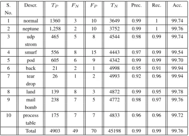
S. Descr. TP FN FP TN Prec. Rec. Acc. No.
1 normal 1360 3 10 3649 0.99 1 99.74 2 neptune 1,258 2 10 3752 0.99 1 99.76 3 udp 465 5 8 4544 0.98 0.99 99.74
strom
4 smurf 556 8 15 4443 0.97 0.99 99.54 5 pod 605 6 9 4342 0.99 0.99 99.70 6 back 21 2 1 4998 0.95 0.91 99.94 7 tear 26 1 2 4993 0.92 0.96 99.94
drop
8 land 139 8 3 4872 0.99 0.95 99.78 9 mail 238 7 5 4772 0.98 0.97 99.76
bomb
10 process 175 7 7 4833 0.96 0.96 99.72 table
Total 4903 49 70 45198 0.99 0.99 99.76
the accuracy of the RBP model over the same dataset is 99.35. It indicates that the accuracy of the proposed model is 0.41 higher than the RBP model. For better visualization, a graphical representation of the comparative analysis is shown in Figure 4. Figure 5 depicts the number of rules generated, number of rules discarded, and the number of rules finally selected for each class. The total number of rules generated are 169, and 18% number of rules are discarded through validation. This results the number of rules minimized to 82%.
Fig. 4: Graphical Presentation of Comparative Analysis
TABLE XVI: Comparative analysis
S. Descr. DRS RBP MCM RBF RAM WTM No. Acc. Acc. Acc. Acc. Acc. Acc.
1 normal 99.74 99.42 97.67 98.45 98.37 98.36 2 neptune 99.76 99.32 97.30 98.71 98.31 98.21 3 udp 99.74 99.35 98.00 98.63 98.75 98.74
strom
4 smurf 99.54 99.41 97.79 99.01 98.59 98.57 5 pod 99.70 99.27 97.61 98.79 99.01 99.00 6 back 99.94 99.40 97.45 99.04 98.45 98.77 7 tear 99.94 99.31 98.11 99.45 98.63 98.45
drop
8 land 99.78 99.56 97.38 98.37 98.67 98.37 9 mail 99.76 99.22 97.32 98.71 98.35 98.44
bomb
10 process 99.72 99.32 97.43 98.84 98.38 98.37 table
Total Acc. 99.76 99.35 97.60 98.80 98.55 98.53
Fig. 5: Graphical view of numbers of rules selected
VI. CONCLUSION
Denial-of-service attack is one of the key security threats in wireless networks. Defending against DoS attack is of prime importance for industries, and internet service providers. To overcome this attack many techniques are proposed by various researchers [5, 6, 8, 9, 11]. In this paper, we propose a model for the detection of denial of service attack in wireless networks using dominance based rough set. The proposed model is analyzed with the help of KDD cup dataset. The total number of rules generated are 169, and 18% number of rules are discarded through validation. This results the number of rules minimized to 82%. Additionally, it is compared with existing techniques and found better accuracy. The accuracy of the proposed model is 99.76 whereas the accuracy of the RBP model is 99.35. This shows that the proposed model is 0.41 higher than the RBP model.
REFERENCES
[1] X. Chuiyi, Z. Yizhi, B. Yuan, L. Shuoshan and X. Qin, A distributed intrusion detection system against flooding denial-of-services attacks, International Conference on Artificial Computing Technology, 2011, pp. 878-881.
[2] X. Ren,(2009)Intrusion detection method using protocol classification and rough set based support vector machine, Computer and Information Science, 2 (2009), pp. 100-108.
[3] R. C. Chen, K. F. Cheng and C. F. Hsieh,Using rough set and support vector machine for network intrusion detection, International Journal of Network Security and Its Applications, 1 (2009), pp. 1-13. [4] Y. Wang,Analysis of a distributed denial of service, Computer Network,
Elsevier, 41 (2009), pp. 1200-1210.
[5] D. Gavrilis and E. Dermatas,Real-time detection of distributed denial-of-service attacks using RBF networks and statistical features, Computer Network, Elsevier, 48 (2005), pp. 235-245.
[6] Y. Wang, C. Lin, Q. L. Li and Y. Fang,A queueing analysis for the denial of service (DoS) attacks in computer networks, Computer Networks, Elsevier, 51 (2007), pp. 3564-3573.
[7] E. Gelenbe and G. Loukas,A self-aware approach to denial of service defence, Computer Networks, Elsevier, 51 (2007), pp. 1299-1314. [8] P. Mell, D. Marks and M. McLarnon, A denial-of-service resistant
intrusion detection architecture, Computer Networks, Elsevier, 34 (2000), pp. 641-658.
[9] M. Hamdi and N. Boudriga, Detecting denial-of-service attacks using the wavelet transform, Computer Networks, Elsevier, 30 (2007), pp. 3203-3213.
[10] S. Chen, Y. Tang and W. Du, Stateful DDoS attacks and targeted filtering, Journal of Network and Computer Applications, Elsevier, 30 (2007), pp. 823-840.
[11] P. A. R. Kumar and S. Selvakumar, Distributed denial of service attack detection using an ensemble of neural classifier, Computer Communication, Elsevier, 30 (2011), pp. 1328-1341.
[12] Z. Pawlak, Rough set: theoretical aspects of reasoning about data, Springer+Business Media, Springer, 1 (1991).
[13] S. Greco, B. Matarazzo and R. Slowinski,The use of rough sets and fuzzy sets in MCDM, In T. Gal, T. Stewart and T. Hanne (eds.) Advances in Multiple Criteria Decision Making, chapter 14, Kluwer Academic Publishers, 1999, pp. 14.1-14.59.
[14] Z. Pawlak, Rough Sets, International Journal of Computer and Information Sciences, 11 (1982), pp. 341-356.
[15] D. B. Parker,Demonstrating the elements of information security with treats, Proceeding of the 17th National Computer Security Conference, 1994, pp. 421-430.
[16] S. Greco, B. Matarazzo and R. Slowinski, J. Stefanowski,An algorithm for induction of decision rules consistent with the dominance principle, European Journalof Operational Research, 117 (1999), pp. 63-83. [17] J. Blaszczynski, S. Greco, B. Matarazzo, R. Slowinski and M. Szelag,
Dominance-based rough set data analysis framework, Users Guide, pp. 1-19.
[18] J. W. Grzymala-Busse, LERS - a system for learning from examples based on rough sets. In R. Slowinski (eds.) Intelligent Decision Support. Handbook of Applications and Advances of the Rough Sets Theory, Kluwer Academic Publishers, Dordrecht, 1992, pp. 3-18.
[19] J. Komorowski, Z. Pawlak, L. Polkowski and A. Skowron,Rough Sets: tutorial. In A. Skowron (eds.) Rough Fuzzy Hybridization. A new trend in decision making, Springer Verlag, Singapore, 1999, pp. 3-98. [20] J. Komorowski,On rough set based approachesto induction of decision
rules. In L. Polkowski, A. Skowron (eds.) Rough Sets in Data Mining and Knowledge Discovery, Physica-Verlag, 1 (1998), pp. 500-529. [21] A. Chonka, W. Zhou, J. Singh and Y. Xiang, Detecting and tracing
distributed denial-of-service attacks by intelligent decision prototype, International Conference on Pervasive Computing and Communications, 1994, pp. 421-430.
[22] J. Yuan and K. Mills,Monitoring the macroscopic effect of distributed denial-of-service flooding attack, IEEE Transactions on Dependable and Secure Computing, 2 (2005), pp. 1-12.
[23] T. Peng, C. Leckie and K. Ramamohanarao,Survey of network-based defense mechanisms countering the DoS and DDoS problems, ACM Computing Surveys, 39 (2007), pp. 370-373.
[24] Y. Qing, W. Xiaoping, L. Yongqing and H. Gaofeng,A hybrid model of RST and DST with its applications in intrusion detection. Interna-tional Symposium on Intelligent Information Technology and Security Information, 2010, pp. 202-205.
[25] R. Shanmugavadivu and N. Nagarajan, Network intrusion detection system using fuzzy logic. Indian Journal of Computer Science and Engineering, 2 (2011), pp. 101-111.