www.the-cryosphere.net/3/57/2009/
© Author(s) 2009. This work is distributed under the Creative Commons Attribution 3.0 License.
The Cryosphere
Comparison of the meteorology and surface energy balance at
Storbreen and Midtdalsbreen, two glaciers in southern Norway
R. H. Giesen1, L. M. Andreassen2,3, M. R. van den Broeke1, and J. Oerlemans1
1Institute for Marine and Atmospheric research Utrecht, Utrecht University, Princetonplein 5, 3584 CC Utrecht, The Netherlands
2Section for Glaciers, Snow and Ice, Norwegian Water Resources and Energy Directorate, P.O. Box 5091 Majorstua, 0316 Oslo, Norway
3Department of Geosciences, University of Oslo, P.O. Box 1047 Blindern, 0316 Oslo, Norway Received: 13 October 2008 – Published in The Cryosphere Discuss.: 17 December 2008 Revised: 5 March 2009 – Accepted: 11 March 2009 – Published: 20 March 2009
Abstract. We compare 5 years of meteorological records from automatic weather stations (AWSs) on Storbreen and Midtdalsbreen, two glaciers in southern Norway, located ap-proximately 120 km apart. The records are obtained from identical AWSs with an altitude difference of 120 m and cover the period September 2001 to September 2006. Air temperature at the AWS locations is found to be highly corre-lated, even with the seasonal cycle removed. The most strik-ing difference between the two sites is the difference in wind climate. Midtdalsbreen is much more under influence of the large-scale circulation with wind speeds on average a factor 1.75 higher. On Storbreen, weaker katabatic winds are dom-inant. The main melt season is from May to September at both locations. During the melt season, incoming and net so-lar radiation are so-larger on Midtdalsbreen, whereas incoming and net longwave radiation are larger on Storbreen, primarily caused by thicker clouds on the latter. The turbulent fluxes are a factor 1.7 larger on Midtdalsbreen, mainly due to the higher wind speeds. Inter-daily fluctuations in the surface energy fluxes are very similar at the AWS sites. On average, melt energy is a factor 1.3 larger on Midtdalsbreen, a result of both larger net radiation and larger turbulent fluxes. The relative contribution of net radiation to surface melt is larger on Storbreen (76%) than on Midtdalsbreen (66%). As win-ter snow depth at the two locations is comparable in most years, the larger amount of melt energy results in an earlier disappearance of the snowpack on Midtdalsbreen and 70% more ice melt than on Storbreen. We compare the relative and absolute values of the energy fluxes on Storbreen and Midtdalsbreen with reported values for glaciers at similar
Correspondence to:R. H. Giesen ([email protected])
latitudes. Furthermore, a comparison is made with meteo-rological variables measured at two nearby weather stations, showing that on-site measurements are essential for an accu-rate calculation of the surface energy balance and melt accu-rate.
1 Introduction
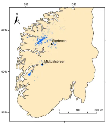
The climate in southern Norway shows a strong precipitation gradient from west to east, with a maritime climate at the western coast and a more continental climate east of the main watershed, located less than 150 km from the coast (Fig. 1, Green and Harding, 1980). The glaciers of southern Norway are found in the areas with the largest annual snow amount; areas characterized by a combination of low temperatures due to topography and sufficient precipitation (Figs. 1 and 2). The annual mass balance turnover (the summed absolute val-ues of the area-averaged winter and summer balance divided by two) on glaciers in southern Norway reflects the precip-itation gradient, ranging from 3.7 m water equivalent (w.e.) at ˚Alfotbreen near the coast to 0.92 m w.e. on Gr˚asubreen in eastern Jotunheimen, further inland. On ˚Alfotbreen, in-terannual fluctuations in the net mass balance are primar-ily determined by variations in the winter balance, while summer-balance variations dominate interannual variability at the more continental glaciers (Andreassen et al., 2005).
��������������� ��������� ������� ������ ����� ����� ����� �����
������ ������� ������� ������� ������� ������� ��������
�������������������������
��
���������� ����������� ����������� ����������� ����������� ���������� ��������� ���������
���������������������������
������������������� ���������� ����������� ���������� ��������� ��������� �������� �������� �����������
���������������������� ������������
� � �
�
� � �
�
� � �
�
Fig. 1. Annual mean air temperature, precipitation and maximum snow amount in southern Norway over the normal period 1971–2000. Note the non-linear scale. The maps are downloaded from seNorge.no, an initiative of the Norwegian Meteorological Institute, the Norwe-gian Water Resources and Energy Directorate and the NorweNorwe-gian Mapping Authority. The locations of Storbreen (S), Midtdalsbreen (M),
˚
Alfotbreen (A) and Gr˚asubreen (G) are indicated on each map.
N
200 km
0 100
5oE
60oN
10oE
62oN
58oN
Storbreen
Midtdalsbreen
Fig. 2. Glaciers in southern Norway (in blue) and the location of Storbreen and Midtdalsbreen. The source for this map is the Statens Kartverk 1:250 000 map series and includes perennial snow fields.
variables and factors, for example wind speed, cloudiness and surface properties. Therefore, detailed knowledge of the relation between meteorological quantities and the mass and energy exchange at the glacier surface can only be obtained from meteorological studies on glaciers. Between 1954 and 1981, glacio-meteorological experiments have been carried out on a number of glaciers in southern Norway (e.g., Li-estøl, 1967; Klemsdal, 1970; Messel, 1971). The combined results from these studies reveal that the relative importance of radiative fluxes compared to turbulent fluxes for surface melt increases from glaciers near the coast to the glaciers fur-ther inland (Messel, 1985). However, a detailed comparison could not be made as the studies were conducted in different years and for different periods during the summer season.
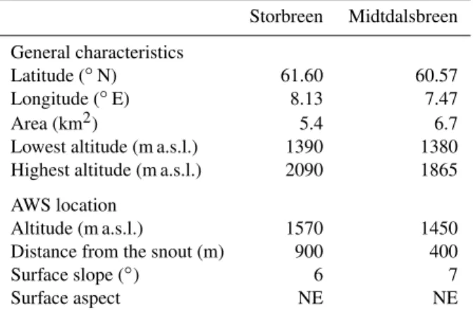
Table 1. The main characteristics of Storbreen and Midtdalsbreen and the AWS sites on the two glaciers. Values are derived from a digital terrain model (DTM) for Storbreen from 1997 (Andreassen, 1999) and a DTM for Hardangerjøkulen from 1995 derived from the 25 m resolution digital terrain model (DTM25) of Norway by the Norwegian mapping authorities (Statens Kartverk, http://www. statkart.no).
Storbreen Midtdalsbreen
General characteristics
Latitude (◦N) 61.60 60.57
Longitude (◦E) 8.13 7.47
Area (km2) 5.4 6.7
Lowest altitude (m a.s.l.) 1390 1380
Highest altitude (m a.s.l.) 2090 1865
AWS location
Altitude (m a.s.l.) 1570 1450
Distance from the snout (m) 900 400
Surface slope (◦) 6 7
Surface aspect NE NE
measured on the two glaciers and discuss their influence on the surface energy balance. In line with previous studies we compare the relative contribution of the surface energy fluxes to melt. The absolute and relative values of the surface en-ergy fluxes are compared with values found for glaciers at similar latitudes, for which we provide a summary which complements earlier overviews (e.g., Ohmura, 2001; Willis et al., 2002; Hock, 2005). To investigate whether similar-ities and differences found for meteorological variables on Storbreen and Midtdalsbreen are also observed outside the glacier boundary-layer, we compare our data with records from two nearby weather stations.
2 Setting and AWS description
Storbreen and Midtdalsbreen are located in southern Norway, 120 km apart (Figs. 2 and 3). Storbreen is a valley glacier in the western part of the Jotunheimen mountain massif. Midt-dalsbreen is an outlet glacier of Hardangerjøkulen, an ice cap situated at the north-western border of the Hardangervidda plateau. Both glaciers are facing north-east, cover a similar altitudinal range and are of comparable size (Table 1). Stor-breen has had a mass deficit since annual mass balance mea-surements started in 1949 (Andreassen et al., 2005). No long-term mass balance series are available for Midtdalsbreen, but annual measurements were initiated in 1963 on Rem-besdalssk˚aka, another outlet glacier from Hardangerjøkulen. They show an approximate equilibrium until the late 1980s and a subsequent mass surplus. After 2000, net mass bal-ances were mainly negative; the net balance of the year 2006 was the lowest ever measured on both Storbreen and Rem-besdalssk˚aka (Kjøllmoen et al., 2007). The net retreat over
the period 1982–2006, when length change was measured at both glaciers, was 80 m at Storbreen and 25 m at Midtdals-breen.
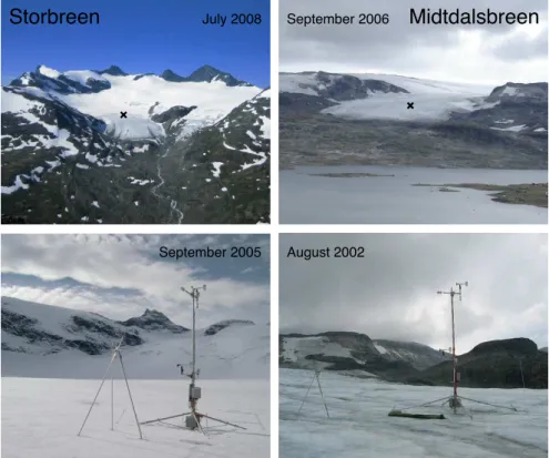
The AWSs on Midtdalsbreen and Storbreen (Fig. 3) are operated by the Institute of Marine and Atmospheric research Utrecht (IMAU). The AWS on Midtdalsbreen was placed in October 2000, the AWS on Storbreen in September 2001. The stations are of identical design and are both located in the ablation zones of the respective glaciers. The mast rests on the ice surface. Air temperature and humidity, wind speed and wind direction are measured at two levels. Temperature and humidity sensors (Vaisala HMP45C) are mounted on the arms at approximately 2.4 and 5.7 m above the ice surface, the measurement level of the wind speed and wind direction sensors (Young 05103) is 0.35 m higher. In addition, the up-per arm carries a radiation sensor (Kipp & Zonen CNR1), measuring the four components of the radiation balance (in-coming and reflected solar radiation, in(in-coming and outgoing longwave radiation), and a sonic ranger (Campbell SR50), measuring the distance to the surface. A second sonic ranger is mounted on a tripod, which is drilled into the ice (Fig. 3). This sonic ranger registers both ice melt and snow accumu-lation. The sonic ranger in the mast ensures a continuous record when the other sensor is buried by snow. Readings at one to four ablation stakes around the AWS are used as a reference for the sonic ranger measurements and enable continuation of the surface height record when data from the sonic rangers is missing. Air pressure (Vaisala PTB101B) is recorded inside the box containing the electronics. Sam-ple time varies per sensor, every 30 min (average) values are stored on a data logger (Campbell CR10X). Power is sup-plied by lithium batteries, the solar panel generates energy to ventilate the temperature sensors.
3 Methods
3.1 Data treatment
In this section we give an overview of the necessary correc-tions to the data. More detailed descripcorrec-tions are given in An-dreassen et al. (2008) and Giesen et al. (2008).
– Air temperature was corrected for radiation errors at times when the sensor was not aspirated using expres-sions that give the excess temperature as a function of wind speed and the sum of incoming and reflected solar radiation.
September 2006 July 2008
September 2005 August 2002
Storbreen
Midtdalsbreen
Fig. 3.The location of the AWSs (×) on Storbreen (left) and Midtdalsbreen (right) and a close-up of the AWS sites. The tripod with a sonic ranger is seen to the left of the mast.
– The sonic ranger uses the speed of sound at 0◦C to
deter-mine the distance to the surface. As the speed of sound is a function of air density and hence temperature, the record was corrected by multiplying with the ratio of the actual speed of sound and the speed of sound at 0◦C. – The tilt of the masts was estimated from tilt angles
mea-sured during maintenance visits, combined with data from a tilt sensor in the mast, which did not function properly. On Midtdalsbreen the estimated tilt of the mast is often large enough to significantly affect the ab-solute value of the incoming solar radiation. The tilt only affects the direct solar beam, hence we applied a tilt correction dependent on cloudiness. A tilted mast also influences the reflected solar radiation measure-ments, but the correction was found to be smaller than uncertainties associated with the poor tilt estimates and was therefore not applied. Tilt values recorded on Stor-breen are smaller and do not seem to influence daily mean values of incoming solar radiation significantly. Hence, no tilt correction was applied to the incoming solar radiation on Storbreen.
– Half-hourly values of net shortwave radiation were cal-culated using the accumulated albedo method (Van den Broeke et al., 2004) to remove the effects of a poor co-sine response of the radiation sensor at low sun angles and a possible phase shift due to tilting of the sensor on
the daily cycle of incoming solar radiation. As we only use daily averaged values in this analysis, the effect of this correction on net shortwave radiation is negligible.
– Due to the opening of a crevasse, the mast on Storbreen fell down in the summer of 2004. The same happened on Midtdalsbreen in 2005. As the data measured dur-ing these periods cannot be used in the analysis, the se-ries from Storbreen contains a 19-day gap from 30 July to 17 August 2004. The series from Midtdalsbreen has 39 days without useful data from 18 July to 25 August 2005. Motivated by the observation that the records of all variables on Storbreen and Midtdalsbreen generally display similar and simultaneous fluctuations, we used measurements from Midtdalsbreen to create a data set to fill the gap on Storbreen. For the data gap on Midt-dalsbreen, we used measurements from an AWS at the summit of Hardangerjøkulen, except for relative humid-ity and incoming longwave radiation where data from Storbreen were used.
the melt season we used melt values calculated from the surface energy balance, combined with stake readings. For Storbreen, measurements from both sonic rangers are lacking during the accumulation season of 2002– 2003. For this period, precipitation data from the nearby Norwegian Meteorological Institute (NMI) weather sta-tion Br˚at˚a (664 m a.s.l.) were used to create a continu-ous record.
3.2 Cloud fraction and effective cloud optical depth Information about clouds can be obtained from both incom-ing shortwave and incomincom-ing longwave radiation. Fractional cloud cover was estimated from incoming longwave radia-tion (Van den Broeke et al., 2008a). Cloud optical thickness was determined from incoming solar radiation using an ex-pression by Fitzpatrick et al. (2004), resulting in effective cloud optical depth values representative for a uniform cloud cover consisting of cloud droplets with a standard effective radius of 8.6 µm. However, this expression can only be ap-plied to daytime measurements without shading by the to-pography. For all days with more than 20 half-hourly values for the cloud optical thickness, we calculated daily averages and regressed these values against the cloud fraction. For both locations, an exponential function fitted the data well (linear correlation r of 0.81) and was used to obtain year-round daily values for cloud optical depth.
3.3 Surface energy balance
The energy balance at the glacier surface can be described by
Q=Sin+Sout+Lin+Lout+Hsen+Hlat+G (1)
=Snet+Lnet+Hsen+Hlat+G, (2)
whereQis melt energy (Q=0 if the surface temperature is below the melting point),SinandSoutare incoming and re-flected solar radiation, Lin andLout are incoming and out-going longwave radiation,HsenandHlatare the sensible and latent heat fluxes andGis the subsurface heat flux. Net solar radiation and net longwave radiation are written asSnet and Lnet. All fluxes are defined positive when directed towards the surface. Heat supplied by rain is neglected, which is jus-tified on glaciers with a considerable mass turnover (Oerle-mans, 2001). Penetration of shortwave radiation is not in-cluded either. Compared to the other fluxes its contribution to the energy balance is expected to be small and it has been shown not to affect total melt (Van den Broeke et al., 2008b).
3.3.1 Model description
We have used an energy balance model that solves Eq. (1) for a skin layer without heat capacity, which is described in more detail by Van den Broeke et al. (2005, 2006). Sin, Sout andLin are taken from the (corrected) measurements,
the other fluxes are written as functions of the surface tem-peratureTs. The model time-step is 10 min, to obtain model input for every time-step, the AWS data are linearly inter-polated between half-hourly values. Using an iterative pro-cedure, the surface energy balance is solved for the surface temperatureTs. IfTs found by the model is higher than the melting point temperature,Tsis set back to 0◦C and the ex-cess energy is used for melting. The amount of meltM in meters water equivalent (m w.e.) is calculated by dividingQ
by the latent heat of fusion (3.34×10⁵J kg−1) and the density of water (1000 kg m−3).
The turbulent fluxes are computed with the bulk method, based on differences in temperature, humidity and wind speed between the measurement level and the surface. We use measurements from the upper level, the records from the lower level sensors contain several data gaps. Following Van den Broeke et al. (2005), stability correction functions by Holtslag and De Bruin (1988) and Dyer (1974) are applied for stable and unstable conditions, respectively. A compar-ison of turbulent fluxes calculated with data from either the upper or the lower measurement level revealed that when us-ing wind speed measurements from the upper level, turbulent fluxes are underestimated, mainly on days with low wind speeds. At both AWS sites, the ratio of wind speeds mea-sured at the upper and lower level is always larger than unity for wind speeds above 6 m s−1; for lower wind speeds this ra-tio is smaller than unity about 20% of the time. On days with a wind speed maximum below the upper level, the wind is always directed down-slope. Moreover, the temperature dif-ference between the air and the surface is mostly larger than 5 K, suggesting the presence of katabatically driven flow. Al-though wind speeds are relatively low in these circumstances, turbulent fluxes are underestimated considerably by using the upper level measurements, because the temperature differ-ence between the air and the surface is large. To obtain good agreement between turbulent fluxes calculated with the up-per or lower level measurements, we limited the turbulent flux reduction by the stability correction to one third when using the upper level data. For the surface roughness length for momentum (z0v) we use constant values of 0.13 mm for
snow surfaces and 0.75 mm for ice surfaces at both AWS sites. Whether the surface is ice or snow is determined from a snow depth record constructed from the sonic ranger mea-surements. The roughness length values are median values, derived from wind speed differences between the AWS upper and lower measurement levels at near-neutral atmospheric conditions. We used the derived roughness lengths for Midt-dalsbreen, as only few datapoints remained for near-neutral conditions at Storbreen and these were mainly found in mid-winter, biasing z0v towards low values. Using roughness
-30 -25 -20 -15 -10 -5 0
-30 -25 -20 -15 -10 -5 0
T s
(modelled,
o C)
Ts(observed, oC)
Midtdalsbreen (b)
-30 -25 -20 -15 -10 -5 0
-30 -25 -20 -15 -10 -5 0
Ts(observed, oC)
T s
(modelled,
o C)
Storbreen (a)
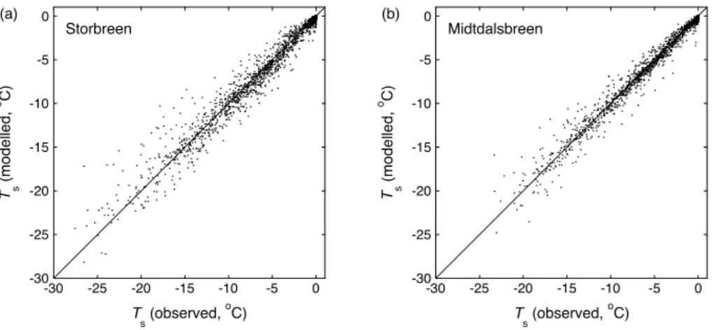
Fig. 4.Modelled versus observed surface temperature (daily mean values) for(a)Storbreen and(b)Midtdalsbreen.
from Midtdalsbreen, have shown that an order-of-magnitude change inz0vroughly affects the sum of the turbulent fluxes
by 15%, while removing the stability correction increases the summed turbulent fluxes by 20%, on average (Giesen et al., 2008). The roughness lengths for heat and moisture are cal-culated from expressions by Andreas (1987).
Subsurface heat conduction is computed from the one-dimensional heat-transfer equation for 0.04 m thick layers down to a depth of 20 m. The temperature at the lowest level is assumed to remain stable. The initial temperature profile is generated by continuously running the model over the mea-surement period until the 20 m temperature is stable within 0.01◦C. The number of snow layers is determined by
divid-ing the observed snow depth by the model layer thickness. Snow density has a constant value of 500 kg m−3, based on measurements in snow pits around the AWSs. Meltwater per-colates vertically through the snowpack and refreezes where snow temperatures are below the melting point. When the snowpack is saturated with melt water, the remaining melt water is assumed to run off. Note that in our approach, the changing snow depth is prescribed from the sonic ranger record and not calculated by the model. This ensures that the snow cover appears and disappears at the right moment. When the snow has disappeared, input from the height sensor is not needed anymore and model and measurements are in-dependent. For this snow-free period, the meltMcomputed by the model can be compared with the surface lowering reg-istered by the sonic ranger and the ablation stakes by divid-ingMby 0.9, the ratio of the ice and water densities used in this study.
3.3.2 Model performance
A comparison of the modelled and observed surface tempera-ture (from measuredLout, assuming a surface with unit emis-sivity) gives an indication of the model performance. Fig-ure 4 shows modelled versus observed daily average surface
temperatures for Storbreen and Midtdalsbreen. The overall agreement is good, although surface temperatures are some-what overestimated on clear-sky winter days. This cannot be attributed to the limited stability correction, removing the limit only slightly reduces the temperature difference on these days. Riming of the sky-facing longwave radiation sensor is a plausible cause. For Storbreen, the mean differ-ence between modelled and observed surface temperature is
+0.07◦C, with a root-mean-square error (RMSE) of 1.3◦C.
For Midtdalsbreen, the mean difference is+0.14◦C with a
RMSE of 1.1◦C. Given the uncertainties in both the
mea-surements and the energy balance model, this is a good re-sult. For both locations, the match between modelled and measured surface melt is generally good (Andreassen et al., 2008; Giesen et al., 2008), which indicates that all relevant processes are included in the model and the calculated energy balance is robust.
4 Results
For the main atmospheric quantities and the surface energy fluxes, mean values over the five years (7 September 2001 to 6 September 2006) were computed, as well as averages over all 30-min intervals when the surface was melting (Q>0). We used measurements made at the upper level for the anal-ysis, since the records from the lower level sensors have sev-eral data gaps. Correlation coefficients (r) between vari-ables on Storbreen and Midtdalsbreen were computed for both half-hourly and daily mean values. The periods with data missing for one of the locations were excluded from the calculation ofr. The mean values and linear correlations are listed in Table 2.
4.1 Air temperature and humidity
Annual mean air temperature is 0.7◦C higher on
-20 -15 -10 -5 0 5 10 15
Storbreen
Air temperature (
o C)
-20 -15 -10 -5 0 5 10 15
Midtdalsbreen
Air temperature (
o C)
-4 -2 0 2 4
1-Jan 1-Jan 1-Jan 1-Jan 1-Jan Storbreen
Midtdalsbreen
Air temperature anomaly (
o C)
2002 2003 2004 2005 2006
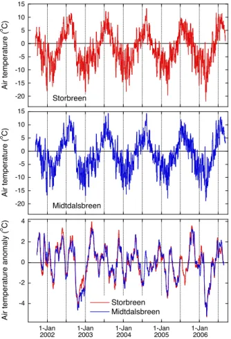
Fig. 5.Daily mean air temperature on Storbreen and Midtdalsbreen and 31-day moving average of daily air temperature anomalies on Storbreen and Midtdalsbreen. The temperature anomalies were cal-culated by subtracting the monthly mean temperature at both loca-tions.
AWS location. The mean and most frequent temperature lapse rate calculated from the two temperature records is 6.0◦C km−1. The temperature difference is smaller during melt (4.3◦C km−1), when the air above the glaciers is cooled by the melting surface. Daily mean air temperatures for the AWS sites on Storbreen and Midtdalsbreen have an almost perfect resemblance, in both inter-daily fluctuations and an-nual amplitude (Fig. 5). The correlation coefficient of daily mean air temperatures on the two glaciers is 0.98 (Table 2). To eliminate the correlation due to the seasonal cycle, we cal-culated daily mean temperature anomalies by subtracting the monthly mean temperature, including all months with mea-surements available from both AWSs. After the removal of the seasonal cycle the linear correlation is still 0.95. Com-puted daily temperature anomalies with a moving average of 31 days, show that the winters 2000–2001, 2002–2003 and 2005–2006 were relatively cold, while the major part of the summer of 2002 was warmer than the other summers in the record (Fig. 5, third panel). In 2003, temperatures in spring were relatively high and 2005 had a very warm autumn.
At both glaciers the air is humid, with an average relative humidity around 80% (Table 2). Relative and specific hu-midity are generally slightly lower on Storbreen. This could indicate a more continental climate than at Midtdalsbreen, but can also be the result of a different boundary-layer struc-ture at the two sites. As the local free-atmosphere humidity is not measured, we cannot distinguish whether the lower hu-midity values on Storbreen are a local or a regional feature. At both AWS sites, specific humidity averaged over the melt season is higher than the annual average, as warmer air can contain more water vapour. The mean relative humidity is also slightly higher in summer than in winter, because the free atmosphere air is cooled near the cold glacier surface, increasing the relative humidity.
4.2 Wind speed and wind direction
The most striking difference between the two glaciers is that wind speeds are on average 1.75 times larger on Midtdals-breen (Table 2). This ratio is almost constant through the year, from October to December values are slightly higher. A similar ratio is found for wind speeds at the lower level, using all available simultaneous wind speed measurements from both locations. The linear correlation between wind speeds at Storbreen and Midtdalsbreen is nonetheless rela-tively high (r=0.74 for daily means).
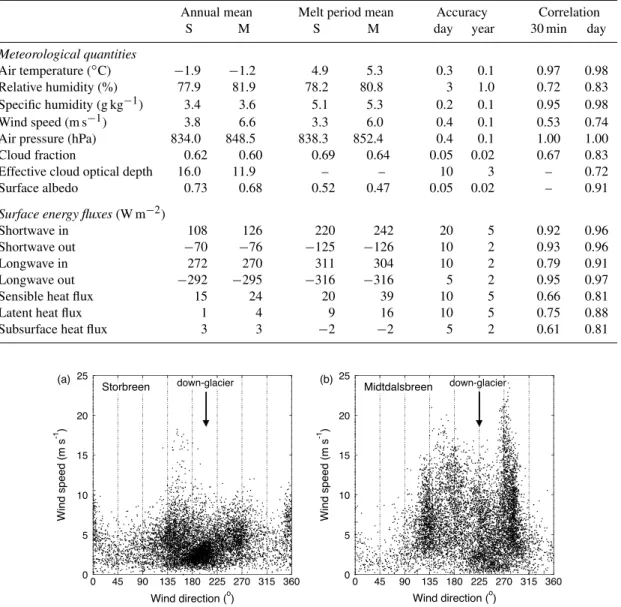
The dominant wind directions on the two glaciers (Fig. 6) are related to the local topography. Two wind directions are imposed by the orientation of the valleys in which the glaciers are situated. Midtdalsbreen flows into the valley Finsedalen, which has an approximate west-east orientation, seen as winds from directions 130◦ and 280◦. Northerly
Table 2.Mean values of meteorological quantities and energy fluxes for Storbreen (S) and Midtdalsbreen (M) over the period 7 September 2001–6 September 2006, for the entire period and periods when the surface was melting. The absolute accuracy is given for daily and annual mean values. Linear correlationsrbetween variables on Storbreen and Midtdalsbreen are shown for half-hourly and daily mean values.
Annual mean Melt period mean Accuracy Correlation
S M S M day year 30 min day
Meteorological quantities
Air temperature (◦C) −1.9 −1.2 4.9 5.3 0.3 0.1 0.97 0.98
Relative humidity (%) 77.9 81.9 78.2 80.8 3 1.0 0.72 0.83
Specific humidity (g kg−1) 3.4 3.6 5.1 5.3 0.2 0.1 0.95 0.98
Wind speed (m s−1) 3.8 6.6 3.3 6.0 0.4 0.1 0.53 0.74
Air pressure (hPa) 834.0 848.5 838.3 852.4 0.4 0.1 1.00 1.00
Cloud fraction 0.62 0.60 0.69 0.64 0.05 0.02 0.67 0.83
Effective cloud optical depth 16.0 11.9 – – 10 3 – 0.72
Surface albedo 0.73 0.68 0.52 0.47 0.05 0.02 – 0.91
Surface energy fluxes(W m−2)
Shortwave in 108 126 220 242 20 5 0.92 0.96
Shortwave out −70 −76 −125 −126 10 2 0.93 0.96
Longwave in 272 270 311 304 10 2 0.79 0.91
Longwave out −292 −295 −316 −316 5 2 0.95 0.97
Sensible heat flux 15 24 20 39 10 5 0.66 0.81
Latent heat flux 1 4 9 16 10 5 0.75 0.88
Subsurface heat flux 3 3 −2 −2 5 2 0.61 0.81
0 5 10 15 20 25
0 45 90 135 180 225 270 315 360 Wind direction (o)
Midtdalsbreen down-glacier (b)
Wind speed (m s
-1 )
0 5 10 15 20 25
0 45 90 135 180 225 270 315 360
Wind speed (m s
-1 )
Wind direction (o) Storbreen down-glacier (a)
Fig. 6.Half-hourly wind speed versus wind direction on(a)Storbreen and(b)Midtdalsbreen. Measurements are shown at hourly intervals for the period September 2005 to September 2006.
4.3 Incoming solar radiation and cloudiness
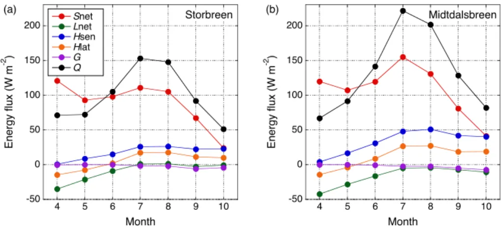
Incoming shortwave radiation is significantly larger on Midt-dalsbreen, both in the annual mean value as in periods with surface melt (Table 2). The annual mean top-of-the-atmosphere incoming solar radiation is only 5 W m−2 higher at Midtdalsbreen, hence the lower latitude of Midt-dalsbreen cannot explain this difference. Figure 7a shows that monthly mean atmospheric transmissivity at the AWS site on Midtdalsbreen is always higher than on Storbreen. On both glaciers, the atmospheric transmissivity is maximum in spring and gradually decreases during summer. The lower atmospheric transmissivity at Storbreen could be caused by
0 5 10 15 20
1 2 3 4 5 6 7 8 9 10 11 12 Storbreen
Midtdalsbreen
Month
Effective cloud optical depth
(b)
0 0.2 0.4 0.6 0.8 1
1 2 3 4 5 6 7 8 9 10 11 12 Storbreen
Midtdalsbreen
Transmissivity
Month (a)
Fig. 7.Monthly mean values of(a)atmospheric transmissivity and(b)effective cloud optical depth on Storbreen and Midtdalsbreen.
variables on Storbreen and Midtdalsbreen, includingSin, are highly correlated, the larger cloud fractions found for Stor-breen are likely associated with local factors affecting cloud properties and not with different synoptic situations at the two glaciers.
4.4 Reflected shortwave radiation and surface albedo Figure 8 presents the daily mean surface albedo for Stor-breen and MidtdalsStor-breen for two winter and summer seasons. These years were selected because the data are continuous and cover two complete seasons. Snow generally starts to accumulate at the AWS sites between the end of September and the end of October. The albedo fluctuations in winter are very similar on the two glaciers. In summer, most precip-itation falls as rain at the AWS sites, but occasional snow-fall events can be recognised by a simultaneous increase in albedo at both locations. In all years, the snow disappears earlier in summer at the AWS site on Midtdalsbreen than on Storbreen. The time difference in ice reappearance at the two locations varies between 11 days (2003) and 35 days (2002) and is weakly related to the maximum snow depth and the difference in total snow accumulation at the two locations. In the winter 2001–2002, Midtdalsbreen received considerably less snow than Storbreen, leading to the largest difference in ice reappearance dates. Ice albedo on Midtdalsbreen re-mained rather high during the summer of 2002 for unknown reasons. In general, ice albedo has a value around 0.3 at both locations, but can get as low as 0.22.
Annual mean reflected shortwave radiation is slightly larger on Midtdalsbreen (+6 W m−2), due to more incoming solar radiation (Table 2). For the period with surface melt, the difference between the two glaciers becomes very small (+1 W m−2), mainly a result of the earlier disappearance of the snowpack on Midtdalsbreen. As the difference between absoluteSoutat the two locations is small,Snet is larger on Midtdalsbreen (Fig. 9).
0 0.2 0.4 0.6 0.8 1
1-Oct 1-Jan 1-Apr 1-Jul 1-Oct 1-Jan 1-Apr 1-Jul 1-Oct Storbreen
Midtdalsbreen
Surface albedo
2002 2003
Fig. 8.Daily mean surface albedo on Storbreen and Midtdalsbreen from October 2001 to October 2003.
4.5 Longwave radiation
Annual mean incoming longwave radiation is comparable at the two AWS locations (Table 2). However, in summer monthly averagedLin is 4 to 6 W m−2larger on Storbreen, while during the winter seasonLin is often larger on Midt-dalsbreen. In summer, thicker clouds on Storbreen result in largerLin than on Midtdalsbreen (Fig. 7b), as was already discussed in Sect. 4.3. The largerLinfor Midtdalsbreen dur-ing the winter months is a result of occasional multi-day peri-ods with substantially more humid and cloudier weather than on Storbreen.
-50 0 50 100 150 200 250
(W m
-2 )
Storbreen
Snet
Lnet -50
0 50 100 150 200 250
Midtdalsbreen
-50 0 50 100
0 50 100 150 200 250 300 350
1-Jan 1-Mar 1-May 1-Jul 1-Sep 1-Nov 1-Jan
2004 2003
-50 0 50 100
(W m
-2 )
Hlat
Hsen
0 50 100 150 200 250 300 350
1-Jan 1-Mar 1-May 1-Jul 1-Sep 1-Nov 1-Jan
(W m
-2 )
2004 2003
Q
G
Fig. 9.Daily mean surface energy fluxes on Storbreen and Midtdalsbreen in 2003.
-50 0 50 100 150 200
4 5 6 7 8 9 10
Snet Lnet Hsen Hlat G Q
Energy flux (W m
-2 )
Month
Storbreen (a)
-50 0 50 100 150 200
4 5 6 7 8 9 10
Month
Energy flux (W m
-2 )
Midtdalsbreen (b)
0 0.2 0.4 0.6 0.8 1
1 2 3 4 5 6 7 8 9 10 11 12
Storbreen Midtdalsbreen
Fraction
Month (a)
-0.5 0 0.5 1 1.5
4 5 6 7 8 9 10
Rnet S
Hsen S
Hlat S G S
Rnet M
Hsen M
Hlat M G M
Month
Fraction
(b)
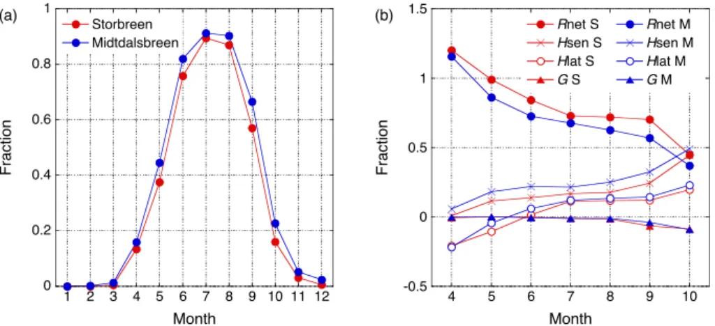
Fig. 11. Monthly values of(a)the fraction of time with melt and(b)the contribution of the energy fluxes to surface melt on Storbreen (S) and Midtdalsbreen (M).
4.6 Turbulent fluxes
On both glaciers, the daily mean sensible heat flux is almost permanently positive (Fig. 9), as the daily average surface temperature is seldom higher than the air temperature. The sensible heat flux is generally larger on Midtdalsbreen, espe-cially in summer, which is a result of the higher air tempera-tures and higher wind speeds.
The latent heat flux is mainly negative and partly balances the sensible heat flux (Fig. 9). Again, the absolute values of Hlat are generally larger on Midtdalsbreen, because of the more humid and windier conditions. During summer, bothHsen andHlat are positive and contribute substantially to the energy available for melting (Fig. 10).
4.7 Subsurface heat flux
The subsurface heat flux warms or cools the surface depend-ing on the sign of the sum of the atmospheric energy fluxes. Daily mean values only occasionally exceed 20 W m−2 and are small compared to the other energy fluxes (Fig. 9). The subsurface heat fluxes are similar in magnitude and inter-daily fluctuations at the two AWS sites. In the early melt season, when the surface consists of snow, G is generally zero or positive as the entire snowpack is at the melting point temperature. As soon as the snow has disappeared, G be-comes slightly negative. The glacier ice is still cold because it was isolated by the snowpack during spring; all through the melt season a small amount of energy is used to warm the ice. The model does not include penetration of shortwave ra-diation, but in reality the near-surface ice is likely heated by penetrating shortwave radiation during the day. This process creates an isothermal layer causingGto vanish.
4.8 Melting energy
The energy available for melting is, on average, a factor 1.3 larger on Midtdalsbreen. Net radiationRnet, the sum of the shortwave and longwave radiative fluxes, is 1.2 times larger
than on Storbreen, the turbulent fluxes are almost twice as large (factor 1.9). On both Storbreen and Midtdalsbreen, the surface is melting almost continuously during July and Au-gust (Fig. 11a). The main melt season is between May and October, whenSnetdominates overLnetand the sum ofHsen andHlatis positive (Fig. 9). In the winter months, melt oc-curs sporadically. During the five years considered in this study, the glacier surface at the AWS site on Storbreen was melting 32% of the time, on Midtdalsbreen this percentage is 35%. The relative contribution of the energy fluxes to the surface melt for the months between April to October is il-lustrated in Fig. 11b. Note that only periods with melt are included in this calculation. In early spring, the contribu-tion ofRnet to surface melt is larger than unity, to balance the negative Hlat. In fact, Snet needs to compensate Hlat and Lnet which are both negative (Fig. 10), implying that largeSin is required for melt in spring. The relative impor-tance ofRnet decreases during the melt season, when top-of-the-atmosphere solar irradiance becomes smaller, cloudi-ness increases and the turbulent fluxes increase due to higher wind speeds. In October,SnetandHsencontribute equally to the melt energy and the turbulent fluxes together dominate the surface energy balance (Figs. 10 and 11b). The largest melt fluxes occur on Midtdalsbreen in July, on Storbreen the amount of melt in July is significantly lower and compara-ble to melt in August. The main cause for this difference is the earlier disappearance of the snowpack on Midtdalsbreen, which happens in June or early July. The lower ice albedo enhances the amount of energy supplied bySnet. Net radia-tion dominates the surface energy balance at both AWS sites, but its relative contribution is larger on Storbreen. Over the entire period with melt its fraction of the total melt energy is 0.76 on Storbreen and 0.66 on Midtdalsbreen.
4.9 Accumulation and ablation
0 1 2 3
Snow depth (m)
-20 -15 -10 -5 0
1-Jan 1-Jan 1-Jan 1-Jan 1-Jan
Storbreen Midtdalsbreen
Surface height (m)
2002 2003 2004 2005 2006
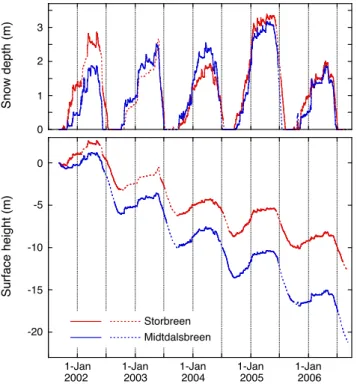
Fig. 12.Daily values of(a)snow depth and(b)cumulative surface height at the AWS sites on Storbreen and Midtdalsbreen for the en-tire period. Direct measurements from the sonic ranger are shown as solid lines, accumulation estimated from precipitation data and ablation computed with the energy balance model are drawn with dashed lines.
AWS sites (Fig. 12a). The similarity between the snow depth records indicates that the two glaciers are situated in a similar precipitation regime, even though Fig. 1 suggests a slightly more maritime climate on Midtdalsbreen. The largest differences between the two records occur when a heavy snowfall event takes place at only one of the two lo-cations. To determine whether these occasional events are related to local or large-scale wind directions, we selected the periods with large differences in snow accumulation. For these periods, we examined both the wind direction mea-sured at the AWS sites as well as the wind direction at the 850 hPa level from (re-)analyses by the European Centre for Medium-Range Weather Forecasts (ECMWF), but no rela-tion was found. On several days with more snowfall on Stor-breen, wind speeds were higher than 10 m s−1on Midtdals-breen, pointing towards fresh snow removal by snowdrift and sublimation. However, during other windy periods on Midt-dalsbreen snow accumulation was similar or higher than on Storbreen, hence no common cause for the snowfall differ-ences could be established.
The larger energy fluxes on Midtdalsbreen lead to a higher ablation rate than on Storbreen. The snowpack on Midt-dalsbreen melts away more quickly in spring, resulting in a longer period with ice at the surface. For the five years considered in this study, the surface became snow-free
be-tween 10 June (in 2002) and 17 July (in 2005) on Midtdals-breen, while on Storbreen the ice reappeared between 4 July (in 2006) and 12 August (in 2005). Over the entire period, the cumulative ice melt is 1.7 times larger on Midtdalsbreen (Fig. 12b). To quantify the effect of the earlier disappear-ance of the snowpack on Midtdalsbreen on the total ice melt, we compared the amount of ice melted in the periods with a snow-free surface at both locations. For these periods, cu-mulative ice melt on Midtdalsbreen is 30% larger than on Storbreen, entirely the result of the larger energy fluxes on Midtdalsbreen. Hence the effect of the earlier reappearance of the ice surface on Midtdalsbreen in the five summers con-sidered, is as large as 40%.
5 Discussion
5.1 Uncertainties in measurements and calculations Meteorological quantities measured on Storbreen and Midt-dalsbreen were found to be generally highly correlated, while absolute differences can be considerable. The identical de-sign of the AWSs minimizes uncertainties due to different instruments, sample intervals or measurement heights. Be-sides uncertainties due to measurement errors, the results from the energy balance model depend on the values chosen for the model parameters. By applying the same model to both data sets, we exclude uncertainties introduced by differ-ent model equations or computation methods. We estimated the accuracy of the measured and modelled variables, con-sidering random and systematic measurement errors as well as uncertainties arising from processing steps and the model design (Table 2). In this section, we discuss the largest error sources and implications for the energy balance calculations. Incoming solar radiation has the largest uncertainty of the measured variables. The instrument accuracy given by the manufacturers is±10% for daily totals (Andreassen et al.,
The effective cloud optical depth calculated from the AWS measurements also has a large uncertainty (Table 2). The parameterization requires solar incoming radiation measure-ments for an unshaded site and can therefore only be deter-mined during daytime when the solar zenith angle is large enough. An exponential relation with daily mean cloud frac-tion values was used to obtain the effective cloud optical depth for all days (Sect. 3.2), including winter days with all-day shading of the AWS site. Although the fitted function describes the relation between cloud fraction and cloud op-tical depth well, large uncertainties are associated with the computed values for individual days.
The largest model uncertainties result from the calcula-tion of the turbulent fluxes, as the available data only provide estimates for the stability correction and the surface rough-ness length, due to the limited number of usable data and the highly variable nature of the surface and the boundary-layer. Giesen et al. (2008) investigated the sensitivity of the turbulent fluxes and modelled melt to changes in the roughness length for momentum and the stability correction. Whenz0v on Midtdalsbreen is increased to 5 mm, the sum
of the mean turbulent fluxes during melt becomes 9 W m−2 higher, while the contribution of the turbulent fluxes to melt increases by 4%. Omitting the stability correction has a sim-ilar effect on the results; applying the full stability correction reduces the absolute and relative contributions to melt by the turbulent fluxes by a comparable magnitude. As the values for z0v and the stability correction used in this study have
been derived from local observations, we expect that these sensitivity tests give the upper limit of uncertainties associ-ated with the turbulent fluxes on Midtdalsbreen. Uncertain-ties in the turbulent fluxes will have a smaller effect on the energy balance at Storbreen, where the turbulent fluxes are less important than on Midtdalsbreen.
Although the uncertainties in the results introduced by measurement errors and model uncertainties are considerable (Table 2), they are mostly smaller than the observed differ-ences in meteorological quantities between the two locations. Hence, it is unlikely that these differences result from mea-surement or model uncertainties.
5.2 Comparison to other glaciers
To compare the surface energy fluxes on Storbreen and Midt-dalsbreen with values on other glaciers, we selected a num-ber of energy balance studies conducted on glaciers at com-parable latitudes, between 50◦and 70◦on both hemispheres.
Table 3 lists the absolute values for the energy fluxes found in these studies and their contribution to the energy balance. The reported values are mostly averages over the measure-ment period and not specifically for a melting surface. How-ever, most studies are conducted during the main melt season and the surface is often assumed or found to be melting con-tinuously. The mean air temperatureTaand wind speedvat the study sites are also listed in Table 3, when reported.
Hu-midity is not included because it is less often reported and cannot be compared directly as some studies report relative and others absolute humidity values.
The mean absolute and relative values for the energy fluxes on Storbreen found in this study are higher than those re-ported for Storbreen for the summer of 1955 (Liestøl, 1967), but the numbers reported for 1955 are within the range of the annual values reported for the period 2001–2006 (An-dreassen et al., 2008). Energy fluxes at the AWS site on Stor-breen compare both in absolute and relative numbers to Mc-Call Glacier (Klok et al., 2005). The total melt energy is also comparable to values reported for Storglaci¨aren (Hock and Holmgren, 1996), Nordbogletscher (Braithwaite and Olesen, 1990) and Omnsbreen (Messel, 1971), but at those loca-tions turbulent fluxes are more important. In fact, Storbreen has the highest contribution by net radiation of all the se-lected studies. A probable explanation is that many of the glaciers in this latitude range are situated in more maritime climates than Storbreen, but the surface albedo on Storbreen may also be lower. In relative numbers, the values found for Midtdalsbreen in this study compare well to those re-ported for Storglaci¨aren, Qamanˆarssˆup sermia (Braithwaite and Olesen, 1990), Ecology Glacier (Bintanja, 1995) and the measurements at 2300 m a.s.l. on Peyto Glacier (Munro, 1990), which were obtained above an ice surface. The abso-lute values for net radiation and total melt energy on Midt-dalsbreen are similar to those measured on Qamanˆarssˆup ser-mia and Peyto Glacier as well, although the values for the separate turbulent fluxes are different. The melting energy on Midtdalsbreen is considerably larger than on Omnsbreen, a small glacier located approximately 11 km north of Midt-dalsbreen. The values for the turbulent fluxes measured on the two glaciers are comparable, but net radiation is much smaller on Omnsbreen. During the investigation period in 1968, Omnsbreen remained snow-covered, in 1969 the ice was not exposed before 21 July (Messel, 1971). The higher surface albedo on Omnsbreen resulted in smaller net radia-tion than during melt periods on Midtdalsbreen.
Table 3. Mean values of the energy fluxes (W m−2) and relative contribution to the surface energy balance (%, boldface numbers) from several energy balance studies. Values are rounded to the nearest integer.Hris heat supplied by rain. The total melt energyQis the sum of the individual energy fluxes, not measured ablation as these are not always equal. When reported, the surface type (snow/firn/ice), altitude (m a.s.l.), mean air temperatureTa(◦C) and wind speedv(m s−1) at the study site are also listed.
Location Latitude Period Surface Ta Rnet Hsen Hlat Hr G Q
Reference Altitude v
McCall Glacier, Alaska 69◦N 15 Jun–20 Aug snow/ice 5.3 93 31 6 – −5 125
(Klok et al., 2005) 2004 1715 3.1 74 25 5 –4
Storglaci¨aren, Sweden 68◦N 19 Jul–27 Aug snow/ice 5.4 73 33 5 – −3 110
(Hock and Holmgren, 1996) 1994 1370 2.5 66 30 5 –3
Qamanˆarssˆup sermia, Greenland 64◦N 1 Jun–31 Aug ice – 103 62 −6 – – 161
(Braithwaite and Olesen, 1990) 1980–1986 790 – 64 39 –4
West Gulkana Glacier, Alaska 63◦N 21 Jun–19 Jul snow/ice – 79 49 11 1 – 139
(Brazel et al., 1992) 1986 1520 – 57 35 8 0
Ecology Glacier, King George Island 62◦S 17 Dec–16 Jan snow/ice 1.9 61 27 7 – – 96
(Bintanja, 1995) 1990–1991 100 5.7 64 29 7
Storbreen, Norway 62◦N 6 Jul–8 Sep snow/ice – 73 40 17 – – 130
(Liestøl, 1967) 1955 1600 – 56 31 13
Storbreen, Norway 62◦N 7 Sep–6 Sep snow/ice 4.9 89 20 9 – −2 117
(this study) 2001–2006 1570 3.3 76 17 8 –2
Nordbogletscher, Greenland 61◦N 1 Jun–31 Aug ice – 79 32 2 – – 111
(Braithwaite and Olesen, 1990) 1979–1983 880 – 71 29 2
Worthington Glacier, Alaska 61◦N 16 Jul–1 Aug ice 9.6 127 68 47 – – 242
(Streten and Wendler, 1968) 1967 ±850 2.1 51 29 20
Omnsbreen, Norway 60◦N 3 Jun–8 Sep snow/ice – 57 35 16 – – 108
(Messel, 1971) 1968–1969 1540 – 52 32 15
Midtdalsbreen, Norway 60◦N 7 Sep–6 Sep snow/ice 5.3 104 39 16 – −2 157
(this study) 2001–2006 1450 6.0 66 25 11 –2
Lemon Creek Glacier, Alaska 58◦N 5 Aug–20 Aug firn 7.6 41 36 8 – – 84
(Wendler and Streten, 1969) 1968 1200 1.5 48 43 9
Koryto Glacier, Russia 55◦N 7 Aug–12 Sep snow 7.6 43 59 31 – – 133
(Konya et al., 2004) 2000 810 2.4 33 44 23
Hodges Glacier, South Georgia 54◦S 1 Nov–4 Apr snow/ice – 47 41 −2 – – 86
(Hogg et al., 1982) 1973–1974 375 3.8 55 48 –3
Glaciar Lengua, Chile 53◦S 28 Feb–12 Apr ice 5.9 57 86 12 7 – 162
(Schneider et al., 2007) 2000 450 4.1 35 54 7 4
Peyto Glacier, Canada 52◦N 17 Jun–6 Jul ice – 108 57 2 – – 166
(Munro, 1990) 1988 2300 – 65 34 1
21 Jun–5 Jul snow – 39 32 5 – – 76
1988 2500 – 51 42 7
Tyndall Glacier, Chile 51◦S 9 Dec–17 Dec ice 5.1 137 111 19 – – 266
(Takeuchi et al., 1995a,b) 1993 700 6.6 51 42 7
Moreno Glacier, Chile 50◦S 12 Nov–27 Nov ice 7.9 139 126 −9 – – 256
(Takeuchi et al., 1995a,b) 1993 330 4.9 54 49 –4
methods are applied to calculate the turbulent fluxes and the contribution of the fluxes to surface melt, which should as well be considered when comparing results. The values re-ported in Table 3 for Storbreen and Midtdalsbreen are av-erages over half-hourly periods with surface melt, as given by the energy balance model. Changing to hourly instead of half-hourly intervals reduced the reported fluxes by 1 to 2%, whereas the relative contributions to melt did not change notably. Although the surface on Storbreen and
Table 4. Mean values and linear correlations of daily mean values of meteorological quantities for Storbreen (S), Sognefjellhytta (So), Midtdalsbreen (M) and Finsevatn (F) over the period 7 September 2001–6 September 2006, for all days with data available for all stations.
Variable Number Coverage Mean Correlation
of days (%) S M So F S–So S–F M–So M–F So–F
Air temperature (◦C) 1518 83 −2.4 −1.7 −2.1 −1.4 0.98 0.92 0.98 0.94 0.97
Relative humidity (%) 927 51 76.4 80.6 83.6 88.3 0.80 0.52 0.78 0.66 0.76
Specific humidity (g kg−1) 805 44 3.0 3.2 3.3 3.6 0.99 0.98 0.98 0.99 0.99
Wind speed (m s−1) 1549 85 3.8 6.6 3.9 5.2 0.70 0.71 0.72 0.90 0.75
Air pressure (hPa) 1305 71 834.0 848.5 850.5 872.9 1.00 0.99 1.00 1.00 1.00
changed by only 1–3% when periods without melt in July and August were included. We conclude that a thorough com-parison between energy fluxes at two different locations can only be made when the period of measurement and the meth-ods applied to determine the turbulent fluxes and the contri-bution to melt are identical, as they are in the present study. 5.3 Comparison to nearby weather stations
As glacio-meteorological records are only available for a limited number of glaciers, mass and energy balance models are mostly driven by meteorological data measured at a dis-tance from the glacier of interest. Although air temperature and air pressure are generally correlated over relatively large distances, variables like wind speed and cloudiness depend on small-scale topography and other local conditions. In this section we compare the records from Storbreen and Midt-dalsbreen with measurements from two NMI weather sta-tions located close to the respective glaciers. Sognefjellhytta (1413 m a.s.l.) is situated 8 km south-west from Storbreen, Finsevatn (1210 m a.s.l.) is located 4 km north-east from the AWS on Midtdalsbreen. Both stations are automatic weather stations with hourly measurements of air temperature, rela-tive humidity, air pressure, wind speed and wind direction. Precipitation is measured at Finsevatn, but is excluded from the comparison as these measurements are very uncertain at automatic weather stations and only snow accumulation is recorded at the AWSs on Storbreen and Midtdalsbreen. Rela-tive humidity measurements were corrected for temperatures below 0◦C (Sect. 3.1). Specific humidity has been calculated
from air temperature, relative humidity and air pressure when these three variables were available. Mean values and linear correlations (r) have been computed for all days with mea-surements from all four stations (Table 4) and are not annual mean values. The relative humidity record from Finsevatn contains large data gaps, hence the number of days included for relative and specific humidity is much smaller than for the other variables.
Daily mean air temperatures at Storbreen, Midtdalsbreen and Sognefjellhytta are highly correlated, while correlations with air temperatures at Finsevatn are considerably lower. On clear-sky days, the diurnal temperature cycle is much
stronger at Sognefjellhytta and Finsevatn than at the glacier sites (Fig. 13). On such days, low wind speeds are recorded outside the glaciers, promoting heating of the near-surface air during the day and strong cooling at night. On the sloping glacier surface, wind speeds are higher and the air is better mixed. Since especially the clear-sky nights are colder out-side the glaciers, mean air temperatures for Sognefjellhytta and Finsevatn are lower than expected from an extrapolation of the mean air temperatures at the glacier sites.
-15 -10 -5 0 5
25 26 27 28 29 30
Storbreen
Midtdalsbreen
Sognefjellhytta
Finsevatn
Air temperature (
o C)
Date (April 2005)
Fig. 13. Hourly air temperatures at Storbreen, Midtdalsbreen, Sognefjellhytta and Finsevatn on six days in April 2005.
depth and surface albedo are taken from the measurements, hence the positive feedback process of a possible change in ice reappearance date on net solar radiation is not included. The model has been run for Storbreen with data from Midt-dalsbreen and Sognefjellhytta, for MidtMidt-dalsbreen we used data from Storbreen and Finsevatn.
Using relative humidity data from another location affects the modelled melt by less than 2%. Applying air temper-atures from the other glacier AWS also has a small effect. However, air temperatures extrapolated from Sognefjellhytta result in 11% more melt on Storbreen and using air temper-atures from Finsevatn lead to an 8% increase in modelled melt on Midtdalsbreen. In spring, applying a different tem-perature record does not notably affect modelled melt, de-spite the large differences in the daily cycle. In summer, air temperatures on the glaciers are almost continuously overes-timated using air temperatures from Sognefjellhytta and Fin-sevatn. The air above the glaciers is cooled by the relatively cold glacier surface and variable lapse rates should be ap-plied. Using wind speeds measured on Midtdalsbreen in the energy balance calculations for Storbreen and vice versa in-duces the largest changes in modelled melt: a 17% increase on Storbreen and a 13% decrease on Midtdalsbreen. Wind speeds from Sognefjellhytta affect the melt on Storbreen by less than 1%, while wind speeds from Finsevatn reduce melt on Midtdalsbreen by 9%. Hence, on glaciers where the tur-bulent fluxes contribute significantly to the total melt, local wind speed and air temperature measurements are required for an accurate calculation of the surface energy balance. Energy balance models driven with data from outside the
glacier boundary-layer need to be calibrated with measure-ments made on the glacier. Alternatively, an energy balance model including glacier boundary-layer processes could be applied (e.g. Denby, 1999).
6 Conclusions
We compared measurements made with two identical AWSs on Storbreen and Midtdalsbreen, two glaciers in southern Norway, 120 km apart. Except for wind speed and wind direction, daily mean values of all recorded variables ex-hibit simultaneous fluctuations of comparable magnitude. Especially daily mean air temperature is highly correlated (r=0.98); the good correlation persists when the seasonal cycle is removed (r=0.95). The average wind speed is a factor 1.75 higher on Midtdalsbreen than on Storbreen. The wind climate on Midtdalsbreen is mainly dominated by the large-scale circulation. On Storbreen, a katabatic wind de-velops regularly and determines the dominant wind direction. Katabatic winds are also observed on Midtdalsbreen, but less frequently, as wind speeds associated with the large-scale cir-culation are much higher. On Midtdalsbreen, westerly winds are dominant.
Incoming and net solar radiation are larger on Midtdals-breen, due to a higher atmospheric transmissivity and an ear-lier disappearance of the snowpack than on Storbreen. In spring and summer, thicker clouds on Storbreen result in more positive incoming and net longwave radiation than on Midtdalsbreen. The turbulent fluxes are a factor 1.9 larger on Midtdalsbreen, mainly due to the larger wind speeds, but secondly because the air is slightly warmer and more humid. On both glaciers net radiation is the largest contributor to surface melt, its relative contribution is larger on Storbreen (76%) than on Midtdalsbreen (66%). The importance of net radiation decreases over the melt season, while the turbulent fluxes become more important. Recorded snow depth at the two AWS sites generally shows simultaneous snowfall events of comparable magnitude. The larger surface energy fluxes on Midtdalsbreen result in a larger ablation rate and an ear-lier reappearance of the ice surface. The consequent drop in albedo further enhances the difference in ablation at the two glaciers; annual ice melt is 70% larger on Midtdalsbreen.
The absolute values and relative contributions of the sur-face energy fluxes to sursur-face melt found for Storbreen and Midtdalsbreen lie within the range of values reported from energy balance studies performed on glaciers at comparable latitudes, although the contribution of net radiation for Stor-breen is relatively large.
Storbreen 0 10 20 30 40 50 60 70 80 90 100 110 120 130 140 150 160 170 180 190 200 210 220 230 240 250 260 270 280 290 300 310 320 330 340350 Midtdalsbreen 0 10 20 30 40 50 60 70 80 90 100 110 120 130 140 150 160 170 180 190 200 210 220 230 240 250 260 270 280 290 300 310 320 330 340350 Sognefjellhytta 0 10 20 30 40 50 60 70 80 90 100 110 120 130 140 150 160 170 180 190 200 210 220 230 240 250 260 270 280 290 300 310 320 330 340350 Finsevatn 0 10 20 30 40 50 60 70 80 90 100 110 120 130 140 150 160 170 180 190 200 210 220 230 240 250 260 270 280 290 300 310 320 330 340350
Fig. 14.Wind direction frequency distributions for Storbreen, Midtdalsbreen, Sognefjellhytta and Finsevatn, where all hourly intervals with measurements at all four stations are included (63% of all hourly intervals).
measurements made on the glacier or should include a glacier-boundary layer model.
Acknowledgements. We thank the IMAU technicians, in particular Wim Boot, for the dedicated maintenance of the AWSs and several colleagues for their assistance in the field. The Norwegian Meteo-rological Institute is thanked for access to and use of their meteo-rological database eKlima. ECMWF ERA-40 and operational data used in this study have been provided by ECMWF. This project has been supported by NWO (Netherlands Organisation for Scientific Research) through the Spinoza-grant to J. Oerlemans.
References
Andreas, E. L.: A theory for the scalar roughness and the scalar transfer coefficients over snow and sea ice, Bound.-Lay. Meteo-rol., 38, 159–184, 1987.
Andreassen, L. M.: Comparing traditional mass balance measure-ments with long-term volume change extracted from topographi-cal maps: a case study of Storbreen glacier in Jotunheimen, Nor-way, for the period 1940–1997, Geogr. Ann. A, 81, 467–476, 1999.
Andreassen, L. M., Elvehøy, H., Kjøllmoen, B., Engeset, R. V., and Haakensen, N.: Glacier mass-balance and length variation in Norway, Ann. Glaciol., 42, 317–325, 2005.
Andreassen, L. M., Van den Broeke, M. R., Giesen, R. H., and Oer-lemans, J.: A 5 year record of surface energy and mass balance from the ablation zone of Storbreen, Norway, J. Glaciol., 54, 245–258, 2008.
Bintanja, R.: The local surface energy balance of the Ecology Glacier, King George Island, Antarctica: measurements and modelling, Antarct. Sci., 7, 315–325, 1995.
Braithwaite, R. J. and Olesen, O. B.: A simple energy-balance model to calculate ice ablation at the margin of the Greenland ice sheet, J. Glaciol., 36, 222–228, 1990.
Brazel, A. J., Tempe, F. B., Chambers, D., and Kalkstein, L. S.: Summer energy balance on West Gulkana Glacier, Alaska, and linkages to a temporal synoptic index, Z. Geomorphol. Suppl. Band, 86, 15–34, 1992.
Curry, J. A. and Webster, P. J.: Thermodynamics of atmospheres and oceans, Academic Press, San Diego, 1999.
Denby, B.: Second-order modelling of turbulence in katabatic flows, Bound.-Lay. Meteorol., 92, 65–98, 1999.
Dyer, A. J.: A review of flux-profile relationships, Bound.-Lay. Me-teorol., 7, 363–372, 1974.
of solar radiation by clouds over snow and ice surfaces: a pa-rameterization in terms of optical depth, solar zenith angle, and surface albedo, J. Climate, 17, 266–275, 2004.
Giesen, R. H., Van den Broeke, M. R., Oerlemans, J., and An-dreassen, L. M.: The surface energy balance in the ablation zone of Midtdalsbreen, a glacier in southern Norway: Interan-nual variability and the effect of clouds, J. Geophys. Res., 113, D21111, doi:10.1029/2008JD010390, 2008.
Green, F. H. W. and Harding, R. J.: The altitudinal gradients of air temperature in southern Norway, Geogr. Ann. A, 62, 29–36, 1980.
Hock, R.: Glacier melt: a review of processes and their modelling, Prog. Phys. Geog., 29, 362–391, 2005.
Hock, R. and Holmgren, B.: Some aspects of energy balance and ablation of Storglaci¨aren, Northern Sweden, Geogr. Ann. A, 78, 121–131, 1996.
Hogg, I. G. G., Paren, J. G., and Timmis, R. J.: Summer heat and ice balances on Hodges Glacier, South Georgia, Falkland Islands Dependencies, J. Glaciol., 28, 221–238, 1982.
Holtslag, A. A. M. and De Bruin, H. A. R.: Applied modeling of the nighttime surface energy balance over land, J. Appl. Meteorol., 27, 689–704, 1988.
Kjøllmoen, B., Andreassen, L. M., Elvehøy, H., Jackson, M., Tvede, A. M., Laumann, T., and Giesen, R. H.: Glaciological investigations in Norway in 2006, NVE Report No 1, Norwegian Water Resources and Energy Directorate, Oslo, 99 pp., 2007. Klemsdal, T.: A glacio-meteorological study of Gr˚asubreen,
Jotun-heimen, in: Norsk Polarinstitutt – ˚Arbok 1968, Norsk Polarinsti-tutt, Oslo, Norway, 58–74, 1970.
Klok, E. J., Nolan, M., and Van den Broeke, M. R.: Analysis of meteorological data and the surface energy balance of McCall Glacier, Alaska, USA, J. Glaciol., 51, 451–461, 2005.
Konya, K., Matsumoto, T., and Naruse, R.: Surface heat balance and spatially distributed ablation modelling at Koryto Glacier, Kamchatka peninsula, Russia, Geogr. Ann. A, 86A, 337–348, 2004.
Liestøl, O.: Storbreen Glacier in Jotunheimen, Norway, Norsk Po-larinstitutt Skrifter Nr. 141, Norsk PoPo-larinstitutt, Oslo, Norway, 63 pp., 1967.
Messel, S.: Mass and heat balance of Omnsbreen – a climatically dead glacier in southern Norway, Norsk Polarinstitutt Skrifter No. 156, Norsk Polarinstitutt, Oslo, Norway, 43 pp., 1971. Messel, S.: Energibalanse-undersøkelser p˚a breer i Norge 1954–
1981, in: Glasiologiske undersøkelser i Norge 1982, NVE rap-port Nr. 1–85, edited by Roland, E. and Haakensen, N., Nor-wegian Water Resources and Energy Directorate, Oslo, Norway, 45–59, 1985.
Munro, D. S.: Comparison of melt energy computations and ab-latometer measurements on melting ice and snow, Arctic Alpine Res., 22, 153–162, 1990.
Oerlemans, J.: Glaciers and Climate Change, Balkema, Lisse, 2001. Ohmura, A.: Physical basis for the temperature-based melt-index
method, J. Appl. Meteorol., 40, 753–761, 2001.
Schneider, C., Kilian, R., and Glaser, M.: Energy balance in the ab-lation zone during the summer season at the Gran Campo Nevado Ice Cap in the Southern Andes, Global Planet. Change, 59, 175– 188, 2007.
Streten, N. A. and Wendler, G.: The midsummer heat balance of an Alaskan maritime glacier, J. Glaciol., 7, 431–440, 1968. Takeuchi, Y., Naruse, R., and Satow, K.: Characteristics of heat
balance and ablation on Moreno and Tyndall glaciers, Patagonia, in the summer 1993/94, Bull. Glacier Res., 13, 45–56, 1995a. Takeuchi, Y., Satow, K., Naruse, R., Ibarzabal, T., Nishida, K., and
Matsuoka, K.: Meteorological features at Moreno and Tyndall glaciers, Patagonia, in the summer 1993/94, Bull. Glacier Res., 13, 35–44, 1995b.
Van den Broeke, M. R., Reijmer, C. H., and Van de Wal, R. S. W.: Assessing and improving the quality of unattended radiation ob-servations in Antarctica, J. Atmos. Ocean. Tech., 21, 1417–1431, 2004.
Van den Broeke, M. R., Reijmer, C. H., Van As, D., Van de Wal, R. S. W., and Oerlemans, J.: Seasonal cycles of Antarc-tic surface energy balance from automaAntarc-tic weather stations, Ann. Glaciol., 41, 131–139, 2005.
Van den Broeke, M. R., Reijmer, C. H., Van As, D., and Boot, W.: Daily cycle of the surface energy balance in Antarctica and the influence of clouds, Int. J. Climatol., 26, 1587–1605, 2006. Van den Broeke, M. R., Smeets, P., Ettema, J., and Kuipers
Munneke, P.: Surface radiation balance in the ablation zone of the west Greenland ice sheet, J. Geophys. Res., 113, doi: 10.1029/2007JD009283, 2008a.
Van den Broeke, M., Smeets, P., Ettema, J., Van der Veen, C., Van de Wal, R., and Oerlemans, J.: Partitioning of melt energy and meltwater fluxes in the ablation zone of the west Greenland ice sheet, The Cryosphere, 2, 179–189, 2008b.
Wendler, G. and Streten, N. A.: A short term heat balance study on a coast range glacier, Pure Appl. Geophys., 77, 68–77, 1969. Willis, I. C., Arnold, N. S., and Brock, B. W.: Effect of snowpack