Evaluation of urban surface parameterizations in the WRF model using measurements during the Texas Air Quality Study 2006 field campaign

(1)

ACPD

10, 25033–25080, 2010

Evaluation of urban surface parameterizations

S.-H. Lee et al.

Title Page

Abstract Introduction

Conclusions References

Tables Figures

◭ ◮

Back Close

Full Screen / Esc

Printer-friendly Version Interactive Discussion

Discussion

P

a

per

|

Dis

cussion

P

a

per

|

Discussion

P

a

per

|

Discussio

n

P

a

per

|

Atmos. Chem. Phys. Discuss., 10, 25033–25080, 2010 www.atmos-chem-phys-discuss.net/10/25033/2010/ doi:10.5194/acpd-10-25033-2010

Atmospheric Chemistry and Physics Discussions

This discussion paper is/has been under review for the journal Atmospheric Chemistry and Physics (ACP). Please refer to the corresponding final paper in ACP if available.

Evaluation of urban surface

parameterizations in the WRF model

using measurements during the Texas Air

Quality Study 2006 field campaign

S.-H. Lee1,2, S.-W. Kim1,2, W. M. Angevine1,2, L. Bianco1,2, S. A. McKeen1,2, C. J. Senff1,2, M. Trainer2, S. C. Tucker1,2,*, and R. J. Zamora2

1

Cooperative Institute for Research in Environmental Sciences, University of Colorado, Boulder, Colorado, USA

2

NOAA Earth System Research Laboratory, Boulder, Colorado, USA

*

now at: Ball Aerospace and Technologies, Corporation, Boulder, Colorado, USA Received: 30 August 2010 – Accepted: 18 October 2010 – Published: 26 October 2010 Correspondence to: S.-H. Lee (sang-hyun.lee@noaa.gov)

(2)

ACPD

10, 25033–25080, 2010

S.-H. Lee et al.

Title Page

Tables Figures

◭ ◮

Back Close

Full Screen / Esc

Discussion

P

a

per

|

Dis

cussion

P

a

per

|

Discussion

P

a

per

|

Discussio

n

P

a

per

|

Abstract

The impact of urban surface parameterizations in the WRF (Weather Research and Forecasting) model on the simulation of local meteorological fields is investigated. The Noah land surface model (LSM), a modified LSM, and a single-layer urban canopy model (UCM) have been compared, focusing on urban patches. The model simula-5

tions were performed for 6 days from 12 August to 17 August during the Texas Air Quality Study 2006 field campaign. Analysis was focused on the Houston-Galveston metropolitan area. The model simulated temperature, wind, and atmospheric boundary layer (ABL) height were compared with observations from surface meteorological sta-tions (Continuous Ambient Monitoring Stasta-tions, CAMS), wind profilers, the NOAA Twin 10

Otter aircraft, and the NOAA Research VesselRonald H. Brown. The UCM simulation showed better results in the comparison of ABL height and surface temperature than the LSM simulations, whereas the original LSM overestimated both the surface temper-ature and ABL height significantly in urban areas. The modified LSM, which activates hydrological processes associated with urban vegetation mainly through transpiration, 15

slightly reduced warm and high biases in surface temperature and ABL height. A comparison of surface energy balance fluxes in an urban area indicated the UCM re-produces a realistic partitioning of sensible heat and latent heat fluxes, consequently improving the simulation of urban boundary layer. However, the LSMs have a higher Bowen ratio than the observation due to significant suppression of latent heat flux. The 20

comparison results suggest that the subgrid heterogeneity by urban vegetation and urban morphological characteristics should be taken into account along with the as-sociated physical parameterizations for accurate simulation of urban boundary layer if the region of interest has a large fraction of vegetation within the urban patch. Model showed significant discrepancies in the specific meteorological conditions when noc-25

(3)

ACPD

10, 25033–25080, 2010

S.-H. Lee et al.

Title Page

Tables Figures

◭ ◮

Back Close

Full Screen / Esc

Discussion

P

a

per

|

Dis

cussion

P

a

per

|

Discussion

P

a

per

|

Discussio

n

P

a

per

|

1 Introduction

Cities occupy less than 0.1% of the whole Earth’s surface, but about 50% of to-tal population inhabits cities. In the Northern America, about 80% of population lived in the urbanized areas in 2003. It is expected that sixty percent of the global population will reside in urban areas by 2030 (UN, 2004). Due to the concentra-5

tion of human activities, most anthropogenic greenhouse gases (e.g. CO2), air pol-lutants, and anthropogenic heat are released from cities, significantly influencing local weather and climate (Crutzen, 2004). Furthermore, population agglomeration in cities makes inhabitants vulnerable to the meteorological and environmental changes such as global/urban warming and poor air quality. Therefore accurate forecasts of local 10

weather and air quality and regional climate change within cities are of primary impor-tance to cope with the issues associated with urbanization.

Urban surfaces are largely composed of artificial buildings and paved roads, there-fore clearly distinguished from natural surfaces (e.g. grassland, there-forest) by mechanical, radiative, thermal, and hydraulic properties. These characteristics in urban morphol-15

ogy can be involved in complicated physical processes such as enhanced momentum drag, radiation trapping within the urban canyon, and efficient heat conduction in the artificial surfaces. The structures of urban boundary layer are influenced by the physi-cal processes over the urban surface. Many field measurements in various cities in the world have shown characteristic features of mean flow, turbulence, thermal structures 20

in the urban canopy layer, urban roughness sublayer, and urban boundary layer (e.g. Dupont et al., 1999; Allwine et al., 2002; Mestayer et al., 2005; Rotach et al., 2005).

Urban numerical modeling has progressed to reproduce the physical processes in an urban area and resultant urban boundary layer structures based on the measure-ments. Generally, an urban patch in land surface models has been represented in an 25

(4)

ACPD

10, 25033–25080, 2010

S.-H. Lee et al.

Title Page

Tables Figures

◭ ◮

Back Close

Full Screen / Esc

Discussion

P

a

per

|

Dis

cussion

P

a

per

|

Discussion

P

a

per

|

Discussio

n

P

a

per

|

natural surfaces. Recently, urban canopy models have been developed with an explicit representation of urban morphology and parameterizations of associated physical pro-cesses (e.g. Masson, 2000; Kusaka et al., 2001; Martilli et al., 2002; Lee and Park, 2008; Oleson et al., 2008). In the models urban physical processes such as in-canyon radiative transfer, turbulence exchanges of momentum, mass, and heat in and above 5

the canyon, and thermal conduction at artificial surfaces are explicitly calculated and interacted. Moreover, various urban surface types can be easily represented by diff er-ent morphological and physical parameters in the models. The inter-comparison study of Grimmond et al. (2010) gives a better description of current urban canopy models and their performance in a stand-alone version.

10

In this study, the urban parameterizations implemented in the meteorological model WRF (Weather Research and Forecasting) are quantitatively evaluated using measure-ments from the second Texas Air Quality Study (TexAQS II) field campaign (Parrish et al., 2009). The measurements include wind fields, temperatures, turbulent fluxes, and atmospheric boundary layer (ABL) heights from several platforms such as surface 15

stations, ship, and aircraft. The intensive observations in time and space allow a faith-ful assessment of the model physics parameterization, consequently giving clues for model physics improvements and overall skill enhancement in the application of air quality simulation. Even though the analysis is focused on quantitative evaluation of ABL processes over the Houston metropolitan area, thorough attention is also paid to 20

the surrounding Galveston Bay and the Gulf of Mexico due to the interactions of the sea/bay breezes and the urban-induced circulation. Complicated interactions of these local circulations characterize the flow patterns of the Houston-Galveston Bay area along with large-scale meteorological forcing conditions (Banta et al., 2005; Tucker et al., 2010). Several numerical simulations have been conducted in the region of interest 25

(5)

ACPD

10, 25033–25080, 2010

S.-H. Lee et al.

Title Page

Tables Figures

◭ ◮

Back Close

Full Screen / Esc

Discussion

P

a

per

|

Dis

cussion

P

a

per

|

Discussion

P

a

per

|

Discussio

n

P

a

per

|

This paper is presented as follows. Section 2 describes the meteorological model WRF and its configuration for the simulations and two urban surface parameterizations based on the Noah land surface model (LSM) and an urban canopy model (UCM). Sim-ple description of the YSU ABL parameterization is also given due to the importance of interpretation of simulation results. Section 3 addresses the measurement data used 5

for the evaluation of the urban surface parameterizations. Comparison results between the simulations and several observations are presented in Sect. 4. Summary and dis-cussions follow in Sect. 5.

2 Model description and configuration

2.1 Mesoscale meteorological model

10

The WRF is a three dimensional, compressible, and non-hydrostatic meteorological model that has been developed by the National Center for Atmospheric Research and several research institutes. It uses an Arakawa-C grid system and a terrain-following pressure coordinate. It includes various physical packages of shortwave and longwave radiative transfer, ABL turbulent mixing, grid-scale cloud physics, cumulus parameteri-15

zation, and land-atmosphere interaction. Several nesting capabilities are also provided. The Advanced Research WRF version 3.1 is used in this study.

Two nested domains are constructed for the simulations in this study. The outer domain has 246×164 mesh with a horizontal resolution of 20 km covering the whole United States (Fig. 1). The inner domain has 226×231 mesh of a 4 km horizontal grid 20

spacing covering the Houston-Galveston areas and Dallas in Texas. The vertical grid is composed of 35 full sigma levels stretching from near surface at about 20 m (the first half sigma level) to the model top (50 hPa). A summary of physical parameterizations used in this study is given in Table 1.

Three simulations with di_fferent urban surface parameterizations are conducted for 25

(6)

ACPD

10, 25033–25080, 2010

S.-H. Lee et al.

Title Page

Tables Figures

◭ ◮

Back Close

Full Screen / Esc

Discussion

P

a

per

|

Dis

cussion

P

a

per

|

Discussion

P

a

per

|

Discussio

n

P

a

per

|

nesting technique. The model ran continuously for the simulation days with a one-day spin-up on 11 August. The National Centers for Environmental Prediction (NCEP) Global Forecast System (GFS) model analysis data with a horizontal resolution of 1◦ are used as meteorological initial and boundary conditions. Analysis is focused on the Houston-Galveston Bay area (Fig. 2).

5

2.2 Urban surface parameterizations

The LSM (Chen and Dudhia, 2001) provides physical bottom boundary conditions to the WRF model. It calculates turbulence exchanges of momentum, mass, and energy between the surface and the overlying atmosphere for governing equations and surface temperature (skin temperature), albedo, and emissivity for radiative transfer equations. 10

Land surface at each grid cell is represented by land-use (vegetation) type and soil textural type, for which the LSM has 24 categorized land-use types and 16 soil textural types. Each land-use type is characterized by physical and aerodynamic parameters such as surface roughness length and displacement height, albedo, emissivity, vege-tation fraction, and leaf area index (LAI), and each soil textural type is characterized 15

by the parameters such as soil heat conductivity and diffusivity, maximum soil moisture content, wilting point soil moisture. Therefore, prescribed physical and aerodynamic parameters are used in computing the turbulence exchanges depending on land-use type and soil type in a model grid cell.

The same approach is applied to urban patches. The LSM does not parameterize 20

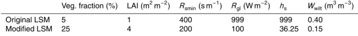
urban physical processes explicitly. Instead, it mimics resultant urban e_ffects by mod-ifying the values of vegetation and soil parameters prescribed for an urban patch. In the original LSM, vegetation fraction and LAI are, for example, set to the values of 10% and 1, respectively. These values are considerably low compared to those for other vegetation types. In addition, high resistances in moisture transfer from the soil surface 25

(7)

ACPD

10, 25033–25080, 2010

S.-H. Lee et al.

Title Page

Tables Figures

◭ ◮

Back Close

Full Screen / Esc

Discussion

P

a

per

|

Dis

cussion

P

a

per

|

Discussion

P

a

per

|

Discussio

n

P

a

per

|

volumetric heat capacity, is set to a relatively large value of 3120 J m−2_K−1_s−1/2 com-pared to those of concrete and asphalt materials (approximately 2000 J m−2_K−1_s−1/2_). These prescribed values of the parameters in the original LSM can highly suppress latent heat flux but enhance sensible heat and storage heat fluxes. Therefore, urban heat island effect can be exaggerated due to significant suppression of hydrological 5

processes in urban areas with urban vegetation.

As many cities in the Unites States, the Houston metropolitan area has a large frac-tion (over 20%) of vegetafrac-tion within the urban area. (Cheng and Byun, 2008). However, the original LSM in WRF cannot accurately consider the effects of the natural surfaces in the urban area as stated above. Therefore, the physical parameters of an urban 10

land-use type need to be modified for the simulation of the model domain in this study. The modification is focused on transpiration enhancement of urban vegetation. In the LSM, the canopy transpiration is calculated using a resistance approach (Jacquemin and Noilhan, 1990). The stomatal resistance Rs for transpiration is controlled by at-mospheric environmental conditions surrounding vegetation and soil wet condition as 15

follows

R_s= Rsmin (LAI)F1F2F3F4

, (1)

where F1, F2, F3, and F4 represent the adjustment factors for incoming solar radia-tion, vapor pressure deficit, air temperature, and soil moisture availability, respectively. These factors are limited to the range of 0 to 1. Rsmin is the minimum stomata re-20

sistance depending on vegetation type. Further, the adjustment factorF1 and F2 are formulated by

F1=

Rsmin/Rsmax+f

(8)

ACPD

10, 25033–25080, 2010

S.-H. Lee et al.

Title Page

Tables Figures

◭ ◮

Back Close

Full Screen / Esc

Discussion

P

a

per

|

Dis

cussion

P

a

per

|

Discussion

P

a

per

|

Discussio

n

P

a

per

|

wheref=0.55_RRg

gl

2 LAI, and

F2=

1

1+hs[qs(Ta)−qa]

, (3)

whereRsmax is the maximum stomata resistance of leaves and is set to 5000 s m− 1

,

Rgis the incoming solar radiation at the surface and the factor of 0.55 is used for the photosynthetically active radiation,Rglis a limit value depending on vegetation type,hs 5

is a non-dimensional coefficient used vapor pressure calculation,qs(Ta) is the saturated water vapor mixing ratio at the air temperatureTa, andqais the air mixing ratio around the vegetation. Details of the parameterization are described in Chen and Dudhia (2001).

For the simulation of the Houston area, we modified the parameters determining tran-10

spiration process in the urban land-use type. The vegetation fraction was assigned as 25% according to the estimation from high resolution land-use mapping data (Cheng and Byun, 2008) and LAI was set to 4. Three land-use type-dependent parameters (Rsmin, Rgl, and hs) associated with transpiration process were changed with corre-sponding values in natural surface land-use types. Finally, the wilting point of soil mois-15

tureWwilt prescribed for an urban patch was reduced from 0.4 m 3

m−3_{to 0.15 m}3_m−3_. This parameter modification activates the transpiration process exerted by the mean vegetation fraction in all urban patches. Modified parameters are listed in Table 2. Cheng and Byun (2008) used similar modification along with additional anthropogenic contribution term in canopy water content equation for the Houston area simulation 20

using MM5 (the fifth generation Pennsylvania State University-National Center for At-mospheric Research Mesoscale Model).

Unlike the traditional approach described above, the UCM used in this study ex-plicitly parameterizes urban physical processes such as in-canyon radiative transfer, turbulence exchanges of momentum, heat, and moisture between the urban surface 25

(9)

ACPD

10, 25033–25080, 2010

S.-H. Lee et al.

Title Page

Tables Figures

◭ ◮

Back Close

Full Screen / Esc

Discussion

P

a

per

|

Dis

cussion

P

a

per

|

Discussion

P

a

per

|

Discussio

n

P

a

per

|

and Cleugh, 1987), in which an urban surface is represented by roof, wall, and road surfaces. Radiation trapping effect within the canyon is parameterized using the sky view factor, albedo, and emissivity at the wall and road surfaces. Surface temperatures at the artificial surfaces are predicted by solving the thermal conduction equations of the roof, wall, and road surfaces. Using the surface temperatures and surrounding 5

air temperatures, sensible heat flux is explicitly calculated at each surface. The urban canopy air temperature is determined diagnostically based on a local thermal equilib-rium assumption. The wind speed required for the calculation of turbulent heat fluxes within the canyon is estimated by a combination of logarithmic profile (above mean building height) and exponential profile (within the canyon). The turbulence exchanges 10

between the urban surface and the overlying atmosphere is calculated using the Monin-Obukhov similarity theory. Detailed formulations can be found in Kusaka et al. (2001).

In addition, the UCM has a capability to represent the subgrid scale variation in an urban grid cell with a separate tile approach (Chen et al., 2004). If artificial surfaces co-exist with natural surfaces in an urban grid, it is represented by a coverage fraction 15

in the model. Therefore, total turbulent fluxes for momentum, heat, and moisture over an urban patch are calculated by

F=fUFU+(1−fU)FN, (4)

wherefU is the fraction of artificial urban surface in an urban patch, and FU and FN indicate the turbulent fluxes from the artificial surface and the natural surface, respec-20

tively. The turbulent flux from the artificial surface FU is calculated in the UCM as a weight-averaged flux of two contributing sources: the roof surface and the canyon, that is,

FU=fRFR+(1−fR)FC, (5)

wherefR is the roof fraction of the whole artificial urban surface, andFR and FC are 25

(10)

ACPD

10, 25033–25080, 2010

S.-H. Lee et al.

Title Page

Tables Figures

◭ ◮

Back Close

Full Screen / Esc

Discussion

P

a

per

|

Dis

cussion

P

a

per

|

Discussion

P

a

per

|

Discussio

n

P

a

per

|

Due to this capability, various urban surface types such as shown in Fig. 3 can be represented with flexibility in the model.

The Houston urban areas are classified into three different classes of commer-cial/industrial area, high density residential area, and low density residential area for the simulation using the National Land Cover Dataset (NLCD) 2001. Figure 2 shows 5

a spatial distribution of dominant land-use type for the nested domain in the Houston-Galveston Bay area. The majority of the urban areas are classified as the low density residential area, and it is surrounded by dryland/cropland/pasture, needle leaf forest, and water bodies (Galveston Bay and the Gulf of Mexico). Physical parameters used for the three urban types are shown in Table 3. Morphological parameters are estimated 10

based on Burian et al. (2003). Urban roughness length and displacement height of each type are calculated in the model using a morphometric method (Macdonald et al., 1998), in which the drag coefficientCDis 1.2 and two empirical constants αm,βm are

4.43, 1.0 respectively. The calculated canyon aspect ratios from mean building height and road width range from 0.25 to 0.67. The sky view factors at the ground range from 15

0.54 in the commercial/industrial area to 0.78 in the low density residential area, which is an important parameter for the radiation trapping effect and is parameterized as a function of canyon aspect ratio in the model. Considering the morphological charac-teristics (Table 3), flow regimes in the Houston areas correspond to wake interference flow or skimming flow (Grimmond and Oke, 1999). Another important parameter used 20

for the simulation of the Houston area is a vegetation fraction that is assigned to 5%, 20%, and 40% for each urban type, respectively. Thermal and radiative parameters for roof, wall, and road surfaces are taken from previous studies (e.g. Kawai et al., 2009).

2.3 Vertical turbulent diffusion parameterization

The vertical turbulent mixing term of the prognostic equation is solved by the Yonsei 25

(11)

ACPD

10, 25033–25080, 2010

S.-H. Lee et al.

Title Page Abstract Introduction Conclusions References Tables Figures ◭ ◮ ◭ ◮ Back Close

Full Screen / Esc

Printer-friendly Version Interactive Discussion Discussion P a per | Dis cussion P a per | Discussion P a per | Discussio n P a per |

performance in a well-mixed atmospheric boundary layer and computational efficiency (e.g. Fast et al., 2006). Here, a brief description of the scheme is given for interpretation of the model simulation results. The vertical turbulent diffusion equation in the mixed layer (z<h) can be expressed as

∂C ∂t =

∂(−wc)

∂z = ∂ ∂z Kc _∂C

∂z −γc

−wch z

h 3

, (6)

5

whereCis the prognostic variables of the model governing equations, K_c is the eddy diffusivity,γ_cis a counter-gradient flux (non-local turbulent mixing),−wchis an

entrain-ment flux at the interfacial layer,zis height above ground level, andhis the ABL height. In the formulation the eddy thermal diffusivity is calculated as

K_θ=P r−1_kw

sz(1−z/h)2, (7)

10

wherek is the von Karman constant, Pr is the turbulence Prandtl number, andw_s is the mixed layer velocity scale. The mixed layer velocity scale is calculated by

ws=(u3∗+8kw 3 ∗z/h)

1/3_,

(8) whereu_∗is the surface friction velocity, w_∗ is the convective velocity scale determined by surface buoyancy flux and ABL height. Therefore, the surface momentum and buoy-15

ancy fluxes and the ABL height are key variables in calculating the eddy diffusivity in the scheme. The ABL height is determined a method based on the surface bulk Richard-son number, in which a height from surface exceeding a critical surface bulk RichardRichard-son number (Rbcr) is found. The surface bulk Richardson number (Rbs) between the surface and a levelz is calculated by

20

Rbs=z

_g

θ0

_θ₍_z₎

−θs

U(z)2 , (9)

(12)

ACPD

10, 25033–25080, 2010

S.-H. Lee et al.

Title Page

Tables Figures

◭ ◮

Back Close

Full Screen / Esc

Discussion

P

a

per

|

Dis

cussion

P

a

per

|

Discussion

P

a

per

|

Discussio

n

P

a

per

|

flux and a mixed layer velocity scale, andU(z) is the horizontal wind speed at a height

z. Di_fferentRbcrare used in the scheme according to the atmospheric stability regime. The YSU scheme uses a value of zero for unstable atmospheric condition and 0.25 for stable atmospheric condition. For free atmosphere above the mixed layer (z>h), the eddy di_ffusivity is calculated based on the localK-closure as in Louis (1979), in which 5

non-local mixing and entrainment processes are ignored.

The YSU scheme in WRF version 3.1 includes several modifications for stable boundary layer that is di_fferent from Hong et al. (2006). One noticeable change is that a parabolic functional form is used in the calculation of eddy diffusivity as is for unstable boundary layer. Another change is thatRbcr for stable ABL height over water 10

bodies is determined as a function of the surface Rossby number following Vickers and Mahrt (2004), instead of a constantRbcr of 0.25. This modification may enhance ver-tical turbulent mixing in stable atmospheric boundary layer compared to the previous version, especially over the land.

3 Observations

15

Quantitative comparison is made for the evaluation of the urban surface parameteri-zations using intensive measurements from surface observation stations, aircraft, and research vessel during the TexAQS II field campaign. The measurements cover the Houston-Galveston Bay area with high resolutions in both space and time. 24 surface stations are used for near surface temperature evaluation. 10 selected surface sta-20

tions among them are used for surface wind field evaluation. These surface stations are mainly located in and around the Houston area. Surface energy balance fluxes at the Brenham and Kirbyville sites are available. These sites are located in the north-western area and northeastern area from Houston, respectively. Several wind profilers were operating during the field campaign (e.g. Wilczak et al., 2009). Wind profiles 25

(13)

ACPD

10, 25033–25080, 2010

S.-H. Lee et al.

Title Page

Tables Figures

◭ ◮

Back Close

Full Screen / Esc

Discussion

P

a

per

|

Dis

cussion

P

a

per

|

Discussion

P

a

per

|

Discussio

n

P

a

per

|

metropolitan area, are also compared with the model results. The wind profiler data were processed using quality control methods (Angevine et al., 1998) and the ABL heights were estimated based on radar reflectivity profiles. Regions of strong signal return are associated with the elevated inversion that caps the convective boundary layer. Following White et al. (1999), the evolution of the ABL was determined by se-5

lecting the height of the peak in reflectivity profiles. Figure 2 shows the location of the surface observation stations.

The NOAA Twin Otter aircraft conducted 22 flights between 1 August and 13 Septem-ber 2006 and covered the Houston-Galveston Bay area, the Dallas-Fort Worth area, and the eastern Texas area. Five flights were done over the Houston-Galveston Bay 10

area during the simulation period. Using the tunable optical profiler for aerosol and ozone lidar (TOPAZ) deployed on the aircraft, profiles of ozone and aerosol concentra-tions in the lower troposphere were measured with 90-m vertical and 600-m horizontal resolutions. The retrieval of the ABL height from these lidar data can be done by de-tecting the maximum gradient of the lidar backscattered data (White et al., 1999; Senff 15

et al., 2002). In this study the estimated ABL height from the aircraft lidar measure-ments is used for the evaluation. Due to wide coverage in and around the Houston areas, these estimates are useful for the evaluation of the impacts of urban surface parameterizations.

During the field campaign, the high-resolution Doppler lidar (HRDL) on the NOAA 20

Research VesselRonald H. Brown was continuously operated. The ship covered ar-eas of the Gulf of Mexico, Galveston Bay, and the Houston Ship Channel. The ship-based HRDL measures horizontal mean wind and turbulence profiles. Based on the measurements, specifically vertical profiles of velocity variance, the ABL heights along ship tracks can be accurately estimated once every 15 minutes (Tucker et al., 2009), 25

(14)

ACPD

10, 25033–25080, 2010

S.-H. Lee et al.

Title Page

Tables Figures

◭ ◮

Back Close

Full Screen / Esc

Discussion

P

a

per

|

Dis

cussion

P

a

per

|

Discussion

P

a

per

|

Discussio

n

P

a

per

|

4 Results

4.1 Surface temperatures and wind fields

The daytime and nighttime 9-h mean observed temperatures for four classified land-use types are given in Table 4. The mean temperature in the commercial/industrial area is higher than that in the high density residential area and the low density residential 5

area by up to 1.5◦_{C in daytime and 1.1}◦_{C in nighttime. When the mean temperature in} the commercial/industrial area is compared to that in the natural surfaces, temperature difference is more distinctive, especially during the nighttime (Table 4). The nighttime mean temperature is higher than that in the natural surfaces by about 1.8◦_{C, indicating} that the vegetated area in the residential areas may have an influence on formation of 10

a nocturnal urban boundary layer.

Figure 4 shows diurnal variations of the observed and simulated 2-m air tempera-tures for each land-use type during the simulation period. The UCM simulation is in better agreement with the observed temperatures than the original LSM simulation for both the residential areas. The UCM well reproduces the observed diurnal variations of 15

2-m temperature including maximum and minimum temperatures, while the LSM over-estimates the temperature in both daytime and nighttime. The observed temperatures in the natural surfaces are well simulated by all the simulations. Therefore, the urban heat island intensity during the nighttime is also better simulated by the UCM than the LSMs. The modified LSM simulation reduces warm biases slightly but the overesti-20

mation remains. For the commercial/industrial area, the simulated temperature by the UCM was lower than the observed temperature by 1–2◦_{C around noon.}

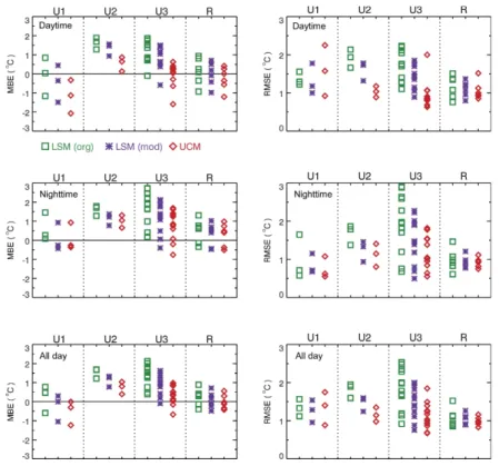
Mean bias error (MBE) and root mean square error (RMSE) of 2-m temperature at 24 stations for the simulation period are shown in Fig. 5. The simulated 2-m temperatures by the LSM show warm biases in most urban stations by up to 2◦_{C in the daytime and} 25

(15)

ACPD

10, 25033–25080, 2010

S.-H. Lee et al.

Title Page

Tables Figures

◭ ◮

Back Close

Full Screen / Esc

Discussion

P

a

per

|

Dis

cussion

P

a

per

|

Discussion

P

a

per

|

Discussio

n

P

a

per

|

and nighttime. Statistics of simulated temperatures with the UCM have the MBE of less than 1.0◦_{C and the RMSE of less than 1.5}◦_{C for most stations during the simulation} period (See the plots for all day in Fig. 5). Furthermore, several stations located in the natural surfaces show improved statistics by urban impacts due to the proximity to the urban areas.

5

Figure 6 compares the simulated 10-m wind fields with the observed during the sim-ulation period. Seven urban stations and three rural stations in and around Houston are averaged (Fig. 2). Statistical evaluation results for each station are presented in Fig. 7. During the first three days from 12 to 14 August, southerly wind was predomi-nant throughout the days. Relatively quick changes in near-surface wind direction due 10

to the influence of sea breeze (bay breeze) are found in the last three days. South-westerly or South-westerly wind near the surface quickly changed to southeasterly or easterly by the intrusion of sea breeze (bay breeze) in the afternoon followed by clockwise ro-tation in wind direction to westerly from late afternoon to early morning (Tucker et al., 2010). This characteristic diurnal rotation in wind direction is partly attributed to the 15

interactions of local circulations and inertial motion due to the Earth’s rotation (Ro-tunno, 1983; Banta et al., 2005). All simulations captured the diurnal variation of the near-surface wind direction throughout the days (Fig. 6a). The MBE of wind direction in each station has a value within 10◦ _{relative to the observed wind direction (Fig. 7).} On the other hand, bias in wind speed is relatively higher than that in wind direction. 20

The daytime wind speed is relatively well simulated by the models, whereas the wind speed is overestimated by up to 1.5 m s−1 _{from late afternoon to early morning.} Dur-ing the nighttime periods, strong winds associated with the nocturnal low-level jet were observed at the La Porte site and from the ship (Tucker et al., 2010). Causes of the nocturnal wind speed bias are explained in Sect. 4.3. Overall performance based on 25

(16)

ACPD

10, 25033–25080, 2010

S.-H. Lee et al.

Title Page

Tables Figures

◭ ◮

Back Close

Full Screen / Esc

Discussion

P

a

per

|

Dis

cussion

P

a

per

|

Discussion

P

a

per

|

Discussio

n

P

a

per

|

4.2 Surface energy balance fluxes

Evaluation of radiative fluxes and turbulent heat fluxes is of primary importance to inter-pret the simulated temperatures and ABL structures. Figure 8 shows the observed and simulated downward shortwave and longwave radiation, sensible heat flux, and latent heat flux at the Brenham site during the simulation period. The site is surrounded by 5

roads, houses, bare grounds, and grasslands. In the model the grid point of the site location is represented as a low density residential area (Fig. 2). The radiative and turbulent fluxes were calculated in an interval of 30 min. The peak downward short-wave radiation exceeds 900 W m−2 _{throughout the days while the longwave radiation} has a value of about 400 W m−2 _{with a small diurnal variation. In the urban patch, the} 10

observed sensible heat and latent heat fluxes show clear diurnal cycles during the sim-ulation period except for 12 August when more cloud cover was present. The sensible heat flux has a peak value of about 300 W m−2_{, and the latent heat flux is lower than} the sensible heat flux by about 60 W m−2_{in the peak time.}

All the models simulate the observed downward shortwave and longwave radiation 15

throughout the days well. Only a small di_fference in radiation is found among the sim-ulations, as expected. In contrast to radiation, the simulated turbulent heat fluxes are significantly different among the simulations, which are caused by different parame-terization of an urban patch. The UCM accurately reproduces the observed sensible heat and latent heat fluxes in magnitude and time. However, the original LSM totally 20

suppresses the latent heat flux, consequently overestimates both the sensible heat flux to the overlying atmosphere and the conductive heat flux into the soil layers during the daytime. These daytime energy partitioning can cause an amplified nocturnal urban heat island effect through the role of the overestimated storage heat flux (Fig. 4). The modified LSM reduces the biases mainly through transpiration process compared to 25

(17)

ACPD

10, 25033–25080, 2010

S.-H. Lee et al.

Title Page

Tables Figures

◭ ◮

Back Close

Full Screen / Esc

Discussion

P

a

per

|

Dis

cussion

P

a

per

|

Discussion

P

a

per

|

Discussio

n

P

a

per

|

energy balance.

Figure 9 shows the comparison of the observed and simulated surface energy bal-ance fluxes at the Kirbyville site, which is located in the northeastern forest area from Houston (Fig. 2). Unlike the Brenham site, the Bowen ratio at this site is less than 1 but downward shortwave and longwave radiative fluxes at the two sites have similar 5

magnitudes. The observed sensible heat flux is simulated quite well by the models, whereas the observed latent heat flux is overestimated. Previous studies with the LSM showed the same bias from the comparison of the observed and simulated latent heat flux in forest areas (Chen et al., 2007; Hong et al., 2009). Due to long distance from the Houston area, the impact of an urban parameterization on the surface energy balance 10

fluxes is insignificant at this site.

4.3 Wind profiles and ABL heights from wind profilers

Figure 10 shows diurnal variations of the observed and simulated wind profiles at the La Porte site on 12 and 16 August. Because the site is located between Houston and Galveston Bay, it is very useful to interpret local circulations associated with contrast of 15

different land-use types. On 12 August, southerly and southwesterly winds in the lowest 1 km were predominant throughout the day (Fig. 10a). In addition, a thick layer with a strong wind speed over 10 m s−1_{(the nocturnal low-level jet) was measured at the site} during the night. The wind direction change due to bay breeze was captured around 18:00 UTC, but local thermal forcing was not enough to overwhelm large scale forcing. 20

In contrast, wind direction changed in accordance with sea/bay breezes development on 16 August. The weak easterly bay breeze formed first around 18:00 UTC with a depth of about 300 m, and then southerly sea breeze with a depth of about 500 m intruded at the site in about 2 h later. This is one of characteristic wind patterns forming in the Houston-Galveston Bay area during the summertime (Nielsen-Gammon, 2002; 25

(18)

ACPD

10, 25033–25080, 2010

S.-H. Lee et al.

Title Page

Tables Figures

◭ ◮

Back Close

Full Screen / Esc

Discussion

P

a

per

|

Dis

cussion

P

a

per

|

Discussion

P

a

per

|

Discussio

n

P

a

per

|

compare well with the observation, especially in wind direction. The simulated sea/bay breezes by the original LSM are stronger and thicker compared to those by the UCM (Figs. 10d-f) because of stronger land-sea thermal contrast in the original LSM.

Figure 11 shows the observed and simulated diurnal variations of wind direction and speed at about 300 m above the ground level at the site during the simulation period. 5

The models well simulate the variation of wind direction throughout the days. The tim-ing of sea/bay breezes at this site is reproduced with an error of an hour or less, except for a slightly larger lag on 17 August. The daytime wind speed is in relatively good agreement with the observation, whereas the nocturnal wind speed is underestimated by the model up to 3 m s−1_{. The bias tends to increase with the wind speed. The} sim-10

ulated wind speed by the UCM is lower by up to 1.5 m s−1_{than that by the LSMs in the} afternoon (approximately 18:00 UTC to 00:00 UTC) when the site is under the influence of sea/bay breezes. This can be explained by the difference in turbulent heat fluxes, especially sensible heat flux, over the Houston metropolitan area shown in Fig. 8. Dur-ing nighttime, the simulated 10-m wind speeds are overestimated as previously shown 15

in Sect. 4.1, while the model winds at 300 m are underestimated, indicating weaker vertical gradients of wind speed for lower atmospheric boundary layer in the model simulations. All simulations fail to capture a strong vertical gradient of the observed wind speed in a layer of several hundred meters above the surface during the night-time. This may be due to excessive vertical turbulent mixing of wind that enhances 20

downward momentum transfer and momentum sink at the surface, consequently flat-tening the vertical profile of wind. The overestimation of nocturnal ABL height can lead to the excessive turbulent mixing because the YSU scheme uses a prescribed parabolic functional form for eddy diffusivity calculation as described in Sect. 2. The possibility that the nocturnal ABL height over land is overestimated in the model will be 25

described in Sect. 4.5. Model discrepancies associated with low-level jets have also reported in the previous studies (e.g. Zhang et al., 2001; Storm et al., 2008).

(19)

ACPD

10, 25033–25080, 2010

S.-H. Lee et al.

Title Page

Tables Figures

◭ ◮

Back Close

Full Screen / Esc

Discussion

P

a

per

|

Dis

cussion

P

a

per

|

Discussion

P

a

per

|

Discussio

n

P

a

per

|

profiler can be calculated with confidence only when the convective boundary layer is well defined (Angevine et al., 2003). Therefore, the comparison is valid for the daytime. The La Porte site is classified in the low density residential area and the Arcola site is in the natural surfaces in the model (Fig. 2). All simulations accurately reproduce the gradual development of the ABL height after breakdown of morning surface inversion at 5

both sites. In addition, the observed rapid decrease of the ABL height in the afternoon with intrusion of sea/bay breezes (15–17 August) is also captured in the simulations. The influence of the urban surface parameterizations is more distinctive at the La Porte site (up to about 300 m) than the Arcola site due to the predominance of southerly and southwesterly winds during the simulation period and the land-use difference between 10

the sites.

4.4 ABL heights from NOAA Twin Otter aircraft

Spatial and temporal distributions of ABL heights measured from the aircraft are com-pared to the simulations in Fig. 13. The flights mainly cover the central and northern areas of Houston, Galveston Bay, and the Gulf of Mexico (right panels) in space and 15

the afternoon period in time. Land-use types along the flight tracks are color coded at the top of each figure (left panels). The observed ABL heights over land have large spatial fluctuations ranging from 1 km to 2 km, whereas the ABL heights over ocean are rather homogeneous with a lower height than over land. In addition, noticeable changes in the ABL height are observed in the transition areas of land-use type, espe-20

cially between urban area and natural surface and between land and water bodies. As expected, a difference among the simulations is conspicuous in and around the urban areas. The original LSM tends to overestimate the observed ABL height, which is as-sociated directly with the overestimation of sensible heat flux in the urban areas. On the other hand, the UCM compares better with the observation than the LSM in the ur-25

(20)

ACPD

10, 25033–25080, 2010

S.-H. Lee et al.

Title Page

Tables Figures

◭ ◮

Back Close

Full Screen / Esc

Discussion

P

a

per

|

Dis

cussion

P

a

per

|

Discussion

P

a

per

|

Discussio

n

P

a

per

|

difference near the urban areas.

Figure 14 shows the statistical comparison of the observed and simulated ABL heights in terms of land-use type. Statistical analysis was done for the three clear days of 14–16 August when cloud influence was relatively insignificant in both the model simulation and observation. The highest mean ABL height was observed in the high 5

density residential area by about 1740 m, which is higher than those in the commer-cial/industrial area and the low density residential area by about 300 m. Meanwhile, the mean ABL heights in the dryland/cropland/grassland and forest areas were 1310 m and 1400 m, respectively. The mean ABL height over the water bodies was 890 m. Among them, the ABL heights in Galveston Bay and the Gulf of Mexico ranged from 10

500 m to 1000 m, whereas the ABL height over small inland lakes exceeded 1000 m. A significant improvement is made by the UCM in all three urban classes compared to the LSM simulations. Especially in both the high density and low density residential areas, the MBE of about 600 m in the original LSM simulation is lowered to about 200 m in the UCM simulation. The RMSEs are also reduced noticeably in the urban patches as 15

shown in Fig. 14. Due to the advection effect from near the urban areas, the MBE and RMSE in two natural patches are also enhanced slightly. The improvements both in the ABL height and in the near surface temperature over the urban areas suggest that the UCM is able to reproduce a realistic urban boundary layer through a reasonable partitioning of surface energy balance fluxes.

20

The generally poor performance over water bodies (Figs. 13 and 14) is further ana-lyzed. Figure 15 shows the vertical distribution of simulated potential temperature by the UCM and the observed and simulated ABL heights near Galveston Bay and the Gulf of Mexico in the flights on 14 and 16 August (left panels). These correspond to about 200 km initial flight path of the days (shaded areas in Fig. 13). It also shows the 25

(21)

ACPD

10, 25033–25080, 2010

S.-H. Lee et al.

Title Page

Tables Figures

◭ ◮

Back Close

Full Screen / Esc

Discussion

P

a

per

|

Dis

cussion

P

a

per

|

Discussion

P

a

per

|

Discussio

n

P

a

per

|

shows a near neutral profile of about 300 K. Thermal internal boundary layer is devel-oped due to cold advection from the bay area. In contrast, the simulated ABL height is significantly suppressed on 16 August when Galveston Bay and the Gulf of Mexico are influenced by warm advection from the inland area in the simulation (Fig. 15b). When the inland warm air moves over Galveston Bay and the near-coastal area in the 5

afternoon, the ABL structure over the water bodies has a multi-layer thermal structure vertically by the combination of the upward sensible heat flux from the ocean (weakly unstable) and the overlying warm advection in the model simulation. This feature is clearly shown in the simulated potential temperature profile at 20:00 UTC on 16 August (right panel in Fig. 15b). The YSU scheme fails to reproduce the observed ABL height 10

over the water on 16 August. The increase ofRbcr, which is a critical parameter in ABL height determination in the YSU scheme, to 0.5 did not improve the performance.

4.5 ABL heights from NOAA Research Vessel

Further comparison is made by using the ship-based lidar ABL height measurements (Tucker et al., 2009) which were available 24 h a day around Galveston Bay and the 15

Gulf of Mexico, unlike the aircraft measurements that were only available during flight times, usually in the late afternoon. Figure 16 shows the observed and simulated ABL heights along the ship tracks (right panels) on 12 and 16 August. Here we focus on the observed ABL heights over Galveston Bay and the Gulf of Mexico (shaded region in the figure). In this region, the observed ABL heights range from 300 m to 800 m throughout 20

the days except for a few points that have the ABL heights greater than 1000 m. Pre-vious studies showed that the area of interest is under weakly unstable atmospheric condition (upward sensible heat flux) during summertime (e.g. Hanna et al., 2006). The simulations show good agreement with the observed ABL heights during the daytime except the nighttime on 12 August (Fig. 16a) and the daytime over Galveston Bay on 25

(22)

ACPD

10, 25033–25080, 2010

S.-H. Lee et al.

Title Page

Tables Figures

◭ ◮

Back Close

Full Screen / Esc

Discussion

P

a

per

|

Dis

cussion

P

a

per

|

Discussion

P

a

per

|

Discussio

n

P

a

per

|

nocturnal winds. The observed ABL heights during the nighttime (03:00–13:00 UTC) are about 300 m homogeneously along the ship channel. However, the simulations overestimate the observation up to about 300 m. This may be due that the noctur-nal boundary layer heights over the surrounding land areas are overestimated by the model. As described in the previous section, the model fails to simulate the ABL height 5

around 17:00 UTC on 16 August when warm advection affects atmospheric boundary layer formation over the water.

On the other hand, the model shows the diurnal evolution of ABL height character-ized over land areas in contrast to the observation in the afternoon (18:00–00:00 UTC) on 16 August when the ship was stationed. This can be explained by the fact that the 10

ship location during the time period is represented as a land patch in the model.

5 Summary and conclusions

The urban land surface parameterizations in the WRF model were quantitatively eval-uated using the measurements during the TexAQS II field campaign. The simulations with an original LSM, a modified LSM, and a single-layer UCM were conducted for 15

the period of 12–17 August 2006, during which intensive measurements from various measurement platforms are available for the model evaluation. The measurements in-clude near surface wind fields and temperatures, surface energy balance fluxes, wind profiles, and ABL heights from wind profilers, the NOAA Twin Otter aircraft, and the NOAARonald H. BrownResearch Vessel. The UCM categorizes the urban areas into 20

three different subclasses which are characterized by different morphological, radiative, and thermal properties. Unlike the original LSM, the UCM explicitly parameterizes the urban physical processes (e.g. in-canyon radiative transfer, turbulence exchanges of momentum and energy, and thermal conduction) and also has a capability to consider subgrid vegetation with its fraction of an urban patch in the surface energy balance. 25

(23)

ACPD

10, 25033–25080, 2010

S.-H. Lee et al.

Title Page

Tables Figures

◭ ◮

Back Close

Full Screen / Esc

Discussion

P

a

per

|

Dis

cussion

P

a

per

|

Discussion

P

a

per

|

Discussio

n

P

a

per

|

representation of the urban areas. The analysis was mainly focused on the Houston-Galveston Bay area.

The UCM showed better performance in the comparisons of ABL height and near surface temperature than the LSM simulations. The original LSM overestimated the observed surface temperature and ABL height significantly in Houston due to the sup-5

pression of latent heat flux. The discrepancy of the LSM in the partitioning of turbulent heat fluxes was confirmed by the comparison with the surface energy fluxes observed in an urban area. The modified LSM slightly reduced model biases in surface tem-perature and ABL height compared to the original LSM, but still had warm surface temperature and high ABL biases. These comparison results suggest that subgrid 10

heterogeneity by urban vegetation and urban morphological characteristics should be taken into account along with the associated parameterization of urban physical pro-cesses for accurate simulation of urban boundary layer in the Houston metropolitan area. This study shows the UCM has a great potential to accurately simulate the ob-served urban boundary layer. Meanwhile, the impacts of the urban parameterization 15

on wind field are relatively small with a difference of less than 10◦_{in wind direction and} 1 m s−1_{in wind speed among the simulations.}

This study identified several model discrepancies associated with atmospheric boundary layer processes. The YSU scheme used in this study reasonably reproduced the observed ABL heights for convective atmospheric boundary layer over land sur-20

faces. However, the models significantly underestimated the ABL heights over Galve-ston Bay and the Gulf of Mexico when relatively warm air advected over the water bodies, especially in the daytime. Another model discrepancy was found in wind field under nocturnal high wind conditions like low-level jets. When relatively high wind speed at low-level (< 1 km) existed, the model underestimated the vertical shear of 25

(24)

ACPD

10, 25033–25080, 2010

S.-H. Lee et al.

Title Page

Tables Figures

◭ ◮

Back Close

Full Screen / Esc

Discussion

P

a

per

|

Dis

cussion

P

a

per

|

Discussion

P

a

per

|

Discussio

n

P

a

per

|

Acknowledgements. The authors would like to thank Bryan Lambeth from the Texas Commis-sion on Environmental Quality (TCEQ) for providing the surface observation data and the La Porte wind profiler data. Song-Yoo Hong from Yonsei University provided helpful comments on the manuscript.

References

5

Allwine, K. J., Shinn, J. H., Streit, G. E., Clawson, K. L., and Brown, M.: Overview of UR-BAN 2000: A multiscale field study of dispersion through an urban environment, Bull. Amer. Meteor. Soc., 83, 521–536, 2002.

Angevine, W. M., Bakwin, P. S., and Davis, K. J.: Wind profiler and RASS measurements compared with measurements from a 450-m-tall tower, J. Atmos. Ocean. Technol., 15, 818–

10

825, 1998.

Angevine, W. M., White, A. B., Senff, C. J., Trainer, M., Banta, R. M., and Ayoub, M. A.: Urban– rural contrasts in mixing height and cloudiness over Nashville in 1999, J. Geophys. Res., 108(D3), 4092, doi:10.1029/2001JD001061, 2003.

Banta, R. M., Senff, C. J., Nielsen-Gammon, J. W., Darby, L. S., Ryerson, T. B., Alvarez, R.

15

J., Sandberg, S. P., Williams, E. J., and Trainer, M.: A bad air day in Houston, Bull. Amer. Meteor. Soc., 86, 657–669, 2005.

Bao, J.-W., Michelson, S. A., McKeen, S. A., and Grell, G. A.: Meteorological evaluation of a weather-chemistry forecasting model using observations from the TEXAS AQS 2000 field experiment, J. Geophys. Res., 110, D21105, doi:10.1029/2004JD005024, 2005.

20

Burian, S. J., Han, W.-S., and Brown, M. J.: Morphological analyses using 3D building databases: Houston, Texas. Los Alamos National Laboratory Final Report, LA-UR-03-8633, 66 pp., 2003.

Chen, F. and Dudhia, J.: Coupling an advanced land-surface-hydrology model with the Penn State-NCAR MM5 modeling system. Part I: Model description and implementation, Mon.

25

Weather Rev., 129, 569–585, 2001.

Chen, F., Kusaka, H., Tewari, M., Bao, J.-W., and Hirakuchi, H.: Utilizing the coupled WRF/LSM urban modeling system with detailed urban classification to simulate the urban heat island phenomena over the greater Houston area, Preprints, Fifth Conference on Urban Environ-ment, Vancouver, BC, Canada, Amer. Meteor. Soc., CD-ROM, 9.11, 2004.

(25)

ACPD

10, 25033–25080, 2010

S.-H. Lee et al.

Title Page

Tables Figures

◭ ◮

Back Close

Full Screen / Esc

Discussion

P

a

per

|

Dis

cussion

P

a

per

|

Discussion

P

a

per

|

Discussio

n

P

a

per

|

Chen, F., Manning, K. W., LeMone, M. A., Trier, S. B., Alfieri, J. G., Roberts, R., Tewari, M., Niyogi, D., Horst, T. W., Oncley, S. P., Basara, J. B., and Blanken, P. D.: Description and evaluation of the characteristics of the NCAR high-resolution land data assimilation system, J. Appl. Meteor. Climat., 46, 694–713, 2007.

Cheng, F.-Y., and Byun, D. W.: Application of high resolution land use and land cover data for

5

atmospheric modeling in the Houston-Galveston metropolitan area, Part I: Meteorological simulation results, Atmos. Environ., 42, 7795–7811, 2008.

Crutzen, P. J.: New directions: The growing urban heat and pollution “island” effect-impact on chemistry and climate, Atmos. Environ., 38, 3539–3540, 2004.

Deardorff, J. W.: Efficient prediction of ground surface temperature and moisture, with inclusion

10

of a layer of vegetation, J. Geophys. Res., 83(C4), 1889–1903, 1978.

Dickinson, R. E., Shaikh, M., Bryant, R., and Graumlich, L.: Interactive canopies for a climate model, J. Climate, 11, 2823–2836, 1998.

Dupont, E., Menut, L., Carissimo, B., Pelon, J., and Flamant, P.: Comparison between atmo-spheric boundary layer in Paris and its rural suburbs during the ECLAP experiment, Atmos.

15

Environ., 33, 979–994, 1999.

Fast, J. D., Gustafson, Jr, W. I., Easter, R. C., Zaveri, R. A., Barnard, J. C., Chapman, E. G., Grell, G. A., and Peckham, S. E.: Evolution of ozone, particulates, and aerosol direct radiative forcing in the vicinity of Houston using a fully coupled meteorology-chemistry-aerosol model, J. Geophys. Res., 111, D21305, doi:10.1029/2005JD006721, 2006.

20

Grell, G. A. and Devenyi, D.: A generalized approach to parameterizing convection com-bining ensemble and data assimilation techniques, Geophys. Res. Lett., 29(14), 1693, doi:10.1029/2002GL015311, 2002.

Grimmond, C. S. B. and Oke, T. R.: Aerodynamic properties of urban areas derived from analysis of surface form, J. Appl. Meteor., 38, 1262–1292, 1999.

25

Grimmond, C. S. B., Blackett, M., Best, M. J., Barlow, J., Baik, J.-J., Belcher, S. E., Bohnen-stengel, S. I., Calmet, I., Chen, F., Dandou, A., Fortuniak, K., Gouvea, M. L., Hamdi, R., Hendry, M., Kawai, T., Kawamoto, Y., Kondo, H., Krayenho_ff, E. S., Lee, S.-H., Loridan, T., Martilli, A., Masson, V., Miao, S., Oleson, K., Pigeon, G., Porson, A., Ryu, Y.-H., Salamanca, F., Shashua-Bar, L., Steeneveld, G.-J., Tombrou, M., Voogt, J., Young, D., and Zhang, N.:

30

The international urban energy balance models comparison project: First results from phase 1, J. Appl. Meteor. Climat., 49, 1268–1292, 2010.

(26)

ACPD

10, 25033–25080, 2010

S.-H. Lee et al.

Title Page

Tables Figures

◭ ◮

Back Close

Full Screen / Esc

Discussion

P

a

per

|

Dis

cussion

P

a

per

|

Discussion

P

a

per

|

Discussio

n

P

a

per

|

years of boundary layer observations over the Gulf of Mexico and its shores, Estuarine Coast. Shelf Sci., 70, 541–550, 2006.

Hong, S., Lakshmi, V., Small, E. E., Chen, F., Tewari, M., and Manning, K. W.: Effects of vegeta-tion and soil moisture on the simulated land surface processes from the coupled WRF/Noah model, J. Geophys. Res., 114, D18118, doi:10.1029/2008JD011249, 2009.

5

Hong, S.-Y., Noh, Y., and Dudhia, J.: A new vertical diffusion package with an explicit treatment of entrainment processes, Mon. Weather Rev., 134, 2318–2341, doi:10.1175/MWR3199.1, 2006.

Jacquemin, B., and Noilhan, J.: Sensitivity study and validation of a land surface parameteriza-tion using the HAPEX-MOBILHY data set, Bound.-Layer Meteor., 52, 93–134, 1990.

10

Kawai, T., Ridwan, M. K., and Kanda, M.: Evaluation of the simple urban energy balance model using selected data from 1-yr flux observations at two cities, J. Appl. Meteor. Climat., 48, 693–715, 2009.

Kusaka, H., Kondo, H., Kikegawa, Y., and Kimura, F.: A simple single-layer urban canopy model for atmospheric models: Comparison with multi-layer and slab models, Bound.-Layer

15

Meteor., 101, 329–358, 2001.

Lee, S.-H., and Park, S.-U.: A vegetated urban canopy model for meteorological and environ-mental modelling, Bound.-Layer Meteor., 126, 73–102, 2008.

Louis, J. F.: A parametric model of vertical eddy fluxes in the atmosphere, Bound.-Layer Me-teor., 17, 187–202, 1979.

20

Macdonald, R. W., Griffiths, R. F., and Hall, D. J.: An improved method for estimation of surface roughness of obstacle arrays. Atmos. Environ., 32, 1857–1864, 1998.

Martilli, A., Clappier, A., and Rotach, M. W.: An urban surface exchange parameterization for mesoscale models, Bound.-Layer Meteor., 104, 261–304, 2002.

Masson, V.: A physically-based scheme for the urban energy budget, Bound.-Layer Meteor.,

25

94, 357–397, 2000.

Mestayer, P. G., Durand, P., Augustin, P., Bastin, S., Bonnefond, J.-M., Benech, B., Camp-istron, B., Coppalle, A., Delbarre, H., Dousset, B., Drobinski, P., Druilhet, A., Frejafon, E., Grimmond, C. S. B., Groleau, D., Irvine, M., Kergomard, C., Kermadi, S., Lagouarde, J.-P., Lemonsu, A., Lohou, F., Long, N., Masson, V., Moppert, C., Noilhan, J., Offerle, B., Oke, T. R.,

30

(27)

ACPD

10, 25033–25080, 2010

S.-H. Lee et al.

Title Page

Tables Figures

◭ ◮

Back Close

Full Screen / Esc

Discussion

P

a

per

|

Dis

cussion

P

a

per

|

Discussion

P

a

per

|

Discussio

n

P

a

per

|

Mlawer, E. J., Taubman, S. J., Brown, P. D., Iacono, M. J., and Clough S. A.: Radiative transfer for inhomogeneous atmosphere: RRTM, a validated correlated-k model for the long-wave, J. Geophys. Res., 102(D14), 16663–16682, doi:10.1029/97JD00237, 1997.

Nielsen-Gammon, J.: Validation of physical processes in MM5 for photochemical model input: The Houston 2000 ozone episode, paper presented at 2002 MM5 Meeting, Univ. Corp. for

5

Atmos. Res., Boulder, Colorado, 24–25 June, 2002.

Oke, T. R. and Cleugh, H. A.: Urban heat storage derived as energy balance residuals, Bound.-Layer Meteor., 39, 233–245, 1987.

Oleson, K. W., Bonan, G. B., Feddema, J., Vertenstein, M., and Grimmond, C. S. B.: An urban parameterization for a global climate model. Part 1: Formulation and evaluation for two cities,

10

J. Appl. Meteor. Climat., 47, 1038–1060, 2008.

Parrish, D. D., Allen, D. T., Bates, T. S., Estes, M., Fehsenfeld, F. C., Feingold, G., Ferrare, R., Hardesty, R. M., Meagher, J. F., Nielsen-Gammon, J. W., Pierce, R. B., Ryerson, T. B., Seinfeld, J. H., and Williams, E. J.: Overview of the Second Texas Air Quality Study (TexAQS II) and the Gulf of Mexico Atmospheric Composition and Climate Study (GoMACCS), J.

15

Geophys. Res., 114, D00F13, doi:10.1029/2009JD011842, 2009.

Rotach, M. W., Vogt, R., Bernhofer, C., Batchvarova, E., Christen, A., Clappier, A., Feddersen, B., Gryning, S.-E., Martucci, G., Mayer, H., Mitev, V., Oke, T. R., Parlow, E., Richner, H., Roth, M., Roulet, Y.-A., Ruffieux, D., Salmond, J. A., Schatzmann, M., and Voogt, J. A.: BUBBLE-an urban boundary layer project, Theor. Appl. Climatol., 81, 231–261, 2005.

20

Rotunno, R.: On the linear theory of the land and sea breeze, J. Atmos. Sci., 40, 1999–2009, 1983.

Sellers, P. J., Randall, D. A., Collatz, G. J., Berry, J. A., Field, C. B., Dazlich, D. A., Zhang, C., Collelo, G. D., and Bounoua, L.: A revised land surface parameterization (SiB2) for atmo-spheric GCMs: Model formulation, J. Climate, 9, 676–705, 1996.

25

Senff, C. J., Banta, R. M., Darby, L. S., Angevine, W. M., White, A., Berkowitz, C., and Doran, C.: Spatial and temporal variations in mixing height in Houston. Final report of TNRCC project F-20, 58 pp., 2002.

Storm, B., Dudhia, J., Basu, S., Swift, A., and Giammanco, I.: Evaluation of the Weather Research and Forecasting model on forecasting low-level jets: Implications for wind energy,

30

Wind Energ., doi:10.1002/we.288, 2008.