Hydrol. Earth Syst. Sci., 17, 2581–2597, 2013 www.hydrol-earth-syst-sci.net/17/2581/2013/ doi:10.5194/hess-17-2581-2013
© Author(s) 2013. CC Attribution 3.0 License.
Geoscientiic
Geoscientiic
Hydrology and
Earth System
Sciences
Open Access
Climate change impacts on maritime
mountain snowpack in the Oregon Cascades
E. A. Sproles1,*, A. W. Nolin1, K. Rittger2, and T. H. Painter2
1College of Earth, Ocean, and Atmospheric Sciences, 104 CEOAS Administration Building, Oregon State University,
Corvallis, OR USA 97331-5503, USA
2Jet Propulsion Laboratory, California Institute of Technology, 4800 Oak Grove Dr, Pasadena, CA USA 91109, USA *currently at: National Health and Environmental Effects Research Laboratory, US Environmental Protection Agency,
Corvallis, OR, USA
Correspondence to:E. A. Sproles ([email protected])
Received: 26 October 2012 – Published in Hydrol. Earth Syst. Sci. Discuss.: 21 November 2012 Revised: 15 May 2013 – Accepted: 27 May 2013 – Published: 9 July 2013
Abstract. This study investigates the effect of projected temperature increases on maritime mountain snowpack in the McKenzie River Basin (MRB; 3041 km2) in the Cas-cades Mountains of Oregon, USA. We simulated the spa-tial distribution of snow water equivalent (SWE) in the MRB for the period of 1989–2009 with SnowModel, a spatially-distributed, process-based model (Liston and Elder, 2006b). Simulations were evaluated using point-based measurements of SWE, precipitation, and temperature that showed Nash-Sutcliffe Efficiency coefficients of 0.83, 0.97, and 0.80, re-spectively. Spatial accuracy was shown to be 82 % using snow cover extent from the Landsat Thematic Mapper. The validated model then evaluated the inter- and intra-year sen-sitivity of basin wide snowpack to projected temperature in-creases (2◦C) and variability in precipitation (±10 %). Re-sults show that a 2◦C increase in temperature would shift the average date of peak snowpack 12 days earlier and decrease basin-wide volumetric snow water storage by 56 %. Snow-pack between the elevations of 1000 and 2000 m is the most sensitive to increases in temperature. Upper elevations were also affected, but to a lesser degree. Temperature increases are the primary driver of diminished snowpack accumula-tion, however variability in precipitation produce discernible changes in the timing and volumetric storage of snowpack. The results of this study are regionally relevant as melt wa-ter from the MRB’s snowpack provides critical wawa-ter sup-ply for agriculture, ecosystems, and municipalities through-out the region especially in summer when water demand is high. While this research focused on one watershed, it serves
as a case study examining the effects of climate change on maritime snow, which comprises 10 % of the Earth’s seasonal snow cover.
1 Introduction
1.1 Significance and motivation
In the mountains of the Western United States, snow water equivalent (SWE, the amount of water stored in the snow-pack) reaches its basin-wide maximum on approximately 1 April (Serreze et al., 1999; Stewart et al., 2004). In the PNW, there have been significant declines in 1 April SWE and accompanying shifts in streamflow have been observed (Service, 2004; Barnett et al., 2005; Mote et al., 2005; Luce and Holden, 2009; Stewart, 2009; Fritze et al., 2011). This reduction in SWE has been attributed to higher winter tem-peratures (Knowles et al., 2006; Mote, 2006; Abatzoglou, 2011; Fritze et al., 2011). Throughout the region, current analyses and those of projected future climate change im-pacts show rising temperatures (Mote and Salath´e, 2010). This increase is expected to transition more snow into rain, resulting in diminished snowpacks, and reduced summer-time streamflow (Service, 2004; Stewart et al., 2004, 2005; Barnett et al., 2005; Mote et al., 2005; Stewart, 2009; Mote and Salath´e, 2010).
This problem is not unique to the Oregon Cascades and is of significance globally as snowmelt provides a sustained source of water for over one billion people (Barnett et al., 2005; Dozier, 2011). The maritime snow class comprises roughly 10 % of the spatial extent of all terrestrial seasonal snow (Sturm et al., 1995) and includes large portions of Japan, Eastern Europe, and the western Cordillera of North America. Many of these regions are mountainous, and mea-surements of snowpack are limited due to complex terrain and sparse observational networks. This deficiency limits the ability to accurately predict snowpack and runoff at the basin scale, especially in a changing climate (Bales et al., 2006; Dozier, 2011). Improvements in quantifying the water stor-age of mountain snowpack in present and projected climates advance the ability to assess climate impacts on hydrologic processes. While climate impacts on mountain snowpack are a global concern, addressing them at the basin-level provides information at a scale that is effective for resource manage-ment strategies (Dozier, 2011).
1.2 Study area
The McKenzie River Basin has an area of 3041 km2 and ranges in elevation from 150 m at the confluence with the Willamette River near the city of Eugene to over 3100 m at the crest of the Cascades. Precipitation increases with el-evation in the MRB. Average annual precipitation ranges from approximately 1000 mm in the lower elevations to over 3500 mm in the Cascade Mountains (Jefferson et al., 2008). With winter air temperatures commonly close to 0◦C, pre-cipitation phase is highly sensitive to temperature and can fall as rain, snow, or a rain-snow mix. In the MRB, the rain-snow transition zone is broad, ranging from 400 to 1200 m, where a transient snowpack commonly accumulates and melts over the course of a winter (Tague and Grant, 2004; Jefferson et al., 2008; Tague et al., 2008). The seasonal snow zone (areas with a distinct accumulation and ablation period) is situated
above 1200 m where deep snows accumulate from Novem-ber through March, increasing their water storage until the onset of melt, on approximately 1 April. In the MRB regions above 1200 m, the underlying basalt geology provides excel-lent aquifer storage that sustains summer flows (Tague and Grant, 2004; Jefferson et al., 2008; Tague et al., 2008; Brooks et al., 2012). Isotopic analysis found that 60–80 % of summer flow in the Willamette River originated from elevations over 1200 m in the Oregon Cascades (Brooks et al., 2012).
The MRB’s “reservoir” of snow above 1200 m is es-pecially important to the greater Willamette River Basin (30 300 km2). While occupying 12 % of the Willamette, the MRB supplies nearly 25 % of the late summer discharge at its confluence with the Columbia River near Portland, Ore-gon (Hulse et al., 2002). Over 70 % of OreOre-gon’s population resides in the Willamette River Basin and the economy and regional ecosystems depend heavily on the Willamette River, especially in summer months when rainfall is sparse. This makes the MRB’s seasonal snowpack a key resource for eco-logical, urban, and agricultural interests and of great inter-est to water resource managers in the MRB and Willamette River Basin.
Monitoring of the MRB’s seasonal snowpack has been conducted for decades; however accurate measurements of basin-wide mountain snowpack do not exist. The present-day monitoring of mountain snowpack uses point-based data from the Natural Resources Conservation Service (NRCS) Snowpack Telemetry (SNOTEL) network covering an eleva-tion range of only 245 m (1267–1512 m) in a basin where snow typically falls at elevations between 750 and 3100 m. While these middle elevations represent roughly 35 % of the basin’s area, they do not quantify SWE at high elevations. Once the snow melts at the monitoring sites, there is no fur-ther information even though snow persists at higher eleva-tions for several weeks. In the past, this limited configuration of SNOTEL sites has functioned successfully in helping pre-dict streamflow (Pagano et al., 2004), however the network was not designed to quantify and evaluate the impacts of pro-jected future climate change at the watershed scale (Molotch and Bales, 2006; Brown, 2009; Nolin et al., 2012). Mean annual temperatures are projected to increase 2◦C by mid-century, potentially limiting the effectiveness of the current monitoring system. These deficiencies underscore the need for a spatially detailed understanding of snow water stor-age at the watershed scale, which would improve water man-agers’ ability to manage this vital resource in the present and plan for future projected temperature changes.
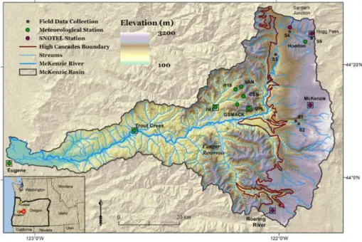
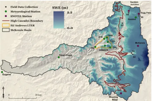
Fig. 1.Context map for the McKenzie River Basin, Oregon. Model forcing locations are enclosed by a black square.
et al., 2009). Such mechanistic snowpack models also al-low us to make projections for future climate scenarios. Re-mote sensing is an effective means of mapping the spatio-temporal character of seasonal snow (Nolin, 2011). Rittger (2012) used a computationally efficient method to compute Fractional Snow Cover Area (fSCA) from Landsat Thematic Mapper in the Sierra Nevada Mountains based on the work of Rosenthal and Dozier (1996) and Painter et al. (2009). Such data are at a spatial scale comparable to topographic and vegetation variations in the MRB and are appropriate for capturing the heterogeneous melt patterns in this watershed. By mapping fSCA, we can obtain an accurate estimate of spatially and temporally varying snow extent, however these data cannot provide estimates of SWE.
Using the MRB as a case study that is representative of mid-latitude maritime snowpacks, this research examines and quantifies the sensitivity of snowpack to climate change. Specifically the research objectives are to: (1) quantify the present-day distribution and volumetric storage of snow wa-ter equivalent at the wawa-tershed scale and across multiple decades; (2) quantify the watershed scale response of snow water equivalent to increases in temperature; and (3) quantify the watershed scale response of snow water equivalent to in-creases in temperature combined with inin-creases or dein-creases in precipitation.
2 Methods
To accomplish these objectives, we applied SnowModel (Lis-ton and Elder, 2006b) to simulate meteorological and snow conditions throughout the McKenzie River Basin at daily
time steps and at a grid resolution of 100 m. The spatially-distributed, process-based model SnowModel computes tem-perature, precipitation, and the full winter season evolution of SWE including accumulation, canopy interception, wind redistribution, sublimation/evaporation, and melt (Liston and Elder, 2006b). The SnowModel framework is comprised of four sub-models. MicroMet provides realistic distributions of air temperature, humidity, precipitation, temperature, wind speed and wind direction, surface pressure, incoming solar and longwave radiation (Liston and Elder, 2006a). The En-Bal sub-model computes the internal energy balance of the snowpack using atmospheric conditions computed by Mi-croMet (Iziomon et al., 2003; Liston and Elder, 2006a, b). SnowTran 3-D is a physically-based snow transport model that distributes the transport and sublimation of snow due to wind (Liston et al., 2007). SnowPack is a single layer sub-model that calculates changes in snow density, depth, and SWE from fluxes in precipitation and melt (Liston and Elder, 2006b). SnowModel was selected because this study required a spatially explicit model that distributes meteorological con-ditions and simulates detailed calculations of the energy bal-ance with a high degree of accuracy. Because SnowModel is physically-based it accounts for slope and aspect in calcu-lating the energy balance, which is especially relevant in the MRB where over 30 % of the basin has slopes greater that 20◦. Additionally the role of land cover (e.g. canopy inter-ception, sublimation, and unloading) is included in the sim-ulations of snowpack evolution. These physical and environ-mental boundary conditions would be lost in a simple degree day model.
Table 1.Meteorological and snow monitoring stations that were applied as model forcings and/or in evaluation of simulation results.Tair
– Air Temperature,P – Precipitation, RH – Relative humidity, Wind – Wind speed and direction, SWE – Snow water equivalent; NWS – National Weather Service, HJA LTER – HJ Andrews Long Term Ecological Research site, NRCS – National Resource Conservation Service.
Used as
Station Measurements model Used in Elevation Run
name used forcing Evaluation (m) by
Eugene Airport Tair,P Yes No 174 NWS
Trout Creek P No Yes 230 NWS
PRIMET Tair,P, RH, Wind, SWE Yes Yes 430 HJA LTER
H15MET Tair,P, RH, Wind No Yes 922 HJA LTER
CENMET Tair,P, RH, Wind, SWE No Yes 1018 HJA LTER
VANMET Tair,P, RH, Wind, SWE No Yes 1273 HJA LTER
UPLMET Tair,P, RH, Wind, SWE Yes Yes 1294 HJA LTER
Santiam Junction Tair,P, SWE No Yes 1267 NRCS
Hogg Pass Tair,P, SWE Yes Yes 1451 NRCS
McKenzie Tair,P, SWE Yes Yes 1454 NRCS
Roaring River Tair,P, SWE Yes Yes 1512 NRCS
direction data as its model forcings. These data were readily available for multiple decades. We applied data from seven automated weather stations distributed throughout the MRB at elevations ranging from 174 to 1512 m (Fig. 1, Table 1). Hypsometrically, 74 % of the area of the McKenzie River Basin is encompassed by the elevation ranges of the monitor-ing sites (430–1512 m), and 85 % of the basin lies below the highest elevation site of 1512 m. While higher elevation me-teorological measurements would have benefitted the study, access to higher elevations was not logistically feasible. A spatially-balanced network of input stations was used to cre-ate a more evenly weighted distribution of forcing data across the watershed (Fig. 1 – stations used as model forcings are enclosed in a black square). The spatially-balanced network was found to be important in distributing precipitation (P ) and air temperature (Tair). The MicroMet sub-model uses the
Barnes Objective Analysis technique, a weighted interpola-tion scheme based on the data spacing from a datum (stainterpola-tion) to the grid cell (Koch et al., 1983). Clusters of stations in the center of the model domain were found to negatively impact model results in the outer regions. The addition of the Eugene Airport improved model agreement by providing a datum in the western portion of the basin. The upper elevation SNO-TEL (National Resource Conservation Service, 2012) sites were added to more evenly distribute meteorological condi-tions in the upper elevacondi-tions. Discussion on how this configu-ration was finalized is discussed in greater detail in the model calibration sub-section.
The study period, WY 1989–2009, was constrained by the availability of meteorological data to drive the model, as stations were required to have a near-complete data record (greater than 90 %). A limited dataset of hourly data for me-teorological stations (10 yr) was available. But because one of our primary objectives was to simulate basin-wide snow-pack over multiple decades, we selected the longer daily time
series. Implementing the hourly forcing data would have de-creased the number of years available for the study by almost 50 % (a full decade). Additionally, the maritime snowpack of the MRB does not have a strong diurnal signal because there is little diurnal variability in air temperature. For example, we calculated the coefficient of variation (CV) for hourly air temperature in WY 2007 and found that 86 % of all days had a CV value that varied by only±2 %. This (and other) mar-itime regions have snowpacks that are warm, nearly isother-mal, and highly sensitive to increased temperature. These characteristics highlight the importance of studies such as this to demonstrate the accumulation and ablation sensitiv-ities of maritime snow. Additionally the study did not fo-cus on the sub-daily/diurnal dynamics of snowpack, which would have required hourly data.
Meteorological data was available through the study pe-riod at 00:00, 06:00, 12:00, 18:00 UTC, and with daily means of air temperature. However, only the 00:00 UTC data from SNOTEL sites are quality assessed (National Resource Con-servation Service, 2013). Test iterations of the model were run with individual inputs for each of these times and results were compared to independent data for goodness of fit and Nash-Sutcliffe Efficiency (NSE) values. The data acquired at 00:00 UTC provided the best goodness of fit and NSE values. We strived to minimize model tuning so we used published values for albedo, albedo decay, and rain-snow temperature partitioning rather than use them as tuning parameters for a better fit with input data from other times of the day. Ad-ditionally, daily precipitation measurements begin and end at 00:00 UTC, which aggregated precipitation to the correct day. Our approach minimized model tuning and allowed a validated model to be run for multiple decades.
(ENSO) for the study period. This time period represents a warm phase of the Pacific Decadal Oscillation (Brown and Kipfmueller, 2012) and compared with records dating back 70 yr, SWE measurements are below the long-term mean (Nolin, 2012).
Physical boundary conditions for the model required el-evation and land cover for the model domain, which was 112 km in the east-west direction and 76 km in the north-south direction. Digital elevation data were obtained from the United States Geological Survey’s (USGS) Seamless Na-tional Elevation Dataset (NED) (Gesch, 2007). The NaNa-tional Land Cover Dataset (NLCD) (Fry et al., 2009) was also ob-tained through USGS. The land cover boundary condition uses vegetation classes (i.e. coniferous forest, barren land), so NLCD land cover types were reclassified to the appro-priate SnowModel land cover code (Sproles, 2012). Both datasets were resampled from 30 m to the model grid resolu-tion of 100 m resoluresolu-tion. Resampling the 30 m data to a grid cell of 100 m captures variability in topography and snow-pack across the landscape, while reducing the computational demands by a factor of eleven. Concerns over potential mis-classification of land cover that may arise from reclassifica-tion are moderated by landscape patterns in the areas where snowfall occurs. These areas are almost entirely coniferous forests in the Western Cascades or unforested, exposed land-scapes in the High Cascades. Any misclassification in resam-pling would most likely only occur at transitional areas. A greater concern regarding land cover is the application of a static land cover dataset over a 21 yr period in a region with a dynamic forest landscape that includes active timber harvest and re-planting. However, developing a dynamic land cover dataset lies outside the scope of this research.
The overall goals of providing spatial and temporal esti-mates of basin-wide SWE across multiple decades were com-pleted in four general steps: (1) apply a physically based, spatially distributed model that uses meteorological data as model forcings; (2) calibrate and validate model outputs of P andTairusing independent station data; (3) calibrate and
validate model outputs of SWE using station data and maps of snow covered area from remote sensing; and (4) conduct a sensitivity analysis of snowpack with regard to temperature and precipitation. Each of these steps is described in greater detail below.
2.1 Model modifications
Two primary modifications were made to SnowModel: a rain/snow precipitation partition function and an albedo de-cay function. These modifications more accurately simulate physical conditions, and improved model performance. The rain/snow precipitation partition function was required be-cause in maritime climates, wintertime temperatures com-monly remain close to 0◦C and mixed phase precipitation events are common. In the PNW, empirical measurements by the United States Army Corps of Engineers (USACE) (1956)
show that the transition from rain to snow exists primarily between a temperature range of−2 to 2◦C. Based upon the USACE study the relationship was implemented in the model using Eq. (1).
SFE=(0.25∗(275.16−Tair))∗P (1)
where, SFE (Snow Fall Equivalent) is the amount of amount of precipitation reaching the ground that falls as snow, Tair
is air temperature in degrees Kelvin, andP is total precipita-tion. Rainfall is computed asP minus SFE. We tested more computationally complex rain-snow algorithms and results were virtually identical. The USACE linear partition pro-vided higher computational efficiency so we proceeded with this approach.
The shortwave albedo of snow (α) has significant effects on surface energy balance, internal energetics, and seasonal evolution of snowpack (Wiscombe and Warren, 1980). Previ-ous versions of SnowModel included snow albedo as a static, tunable parameter (Liston and Elder, 2006b). This study ap-plied an improved snow albedo decay function from Strack et al. (2004) where:
for non-melting conditions
αt =(αt−1−grnm) (2)
and, for melting snow
αt =(αt−1−αmin)∗exp(−grm)+αmin (3)
Whereαt is the snow albedo value used at each time step by
the model in energy balance calculations,αt−1represents the
snow albedo at the previous time step, and the decay gradient is represented by grm= 0.018, grnm= 0.008 for melting and
non-melting conditions, respectively. The maximum albedo value after new snowfall (when new snow depth≥2.5 cm) is set to 0.8 in unforested areas and to 0.6 in forested areas (Burles and Boon, 2011). A minimum snow albedo (αmin)
was set to 0.5 in unforested areas and 0.2 in forested areas. We understand that applying a single albedo decay function has its limitations, and does not account for variation in land cover or topographic effects (Molotch et al., 2004). This po-tential source of model error is addressed in the Discussion.
2.2 Model calibration
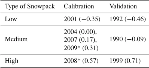
Table 2.Water years used in the calibration and validation of the model. Selected Values in parentheses represent the deviation from the mean (in meters) of peak SWE measurements at Santiam Junc-tion, Hogg Pass, Roaring River, and McKenzie. Years noted by an * represent years with field measurements of SWE.
Type of Snowpack Calibration Validation
Low 2001 (−0.35) 1992 (−0.46)
Medium
2004 (0.00),
1990 (−0.09) 2007 (0.17),
2009* (0.31)
High 2008* (0.57) 1999 (0.71)
The initial phase focused on optimizing the spatially-distributed gridded values of dailyP andTair. Because
me-teorological conditions are first order controls on snowpack accumulation and ablation, maximizing the accuracy of these spatially interpolated and temporally varying model forcings is an important first step. Without accurate inputs, the result-ing snowpack might be calibrated to correct values, but not for the right reasons (Kirchner, 2006). The second phase fo-cused on optimizing simulations of snowpack. Model eval-uation used point-based measurements for SWE and Land-sat fSCA remote-sensing data for snow cover extent, pro-viding a robust means of model calibration and validation (Andersen and Bates, 2001). Prior to the implementation of the albedo decay function and rain-snow partition, there was an overestimation of modeled snow extent compared to the point-based measurements and remote-sensing data. How-ever, once these modifications were incorporated into the model, spatial agreement improved considerably. This im-provement makes sense conceptually. The fixed rain-snow partition simulated 100 % of precipitation to fall as snow when air temperature was 2◦C or colder, and lead to an over-estimation of snow. Compounding this overover-estimation was a fixed albedo that underestimated shortwave energy critical to the melt process. The rain-snow partition would propor-tion less precipitapropor-tion falling as snow, and the albedo decay would hasten the melt process.
The optimal configuration of meteorological stations was determined by iteratively adding individual stations in the model. Results of each iteration were compared to stations independent of those used in the model (Table 1) using met-rics described later in the next section. Paired sets of wa-ter years with statistically high, low, and average peak SWE were used to calibrate and validate the model (Table 2). Cali-bration was performed on the first set of water years, and then validated to the second set of water years. Once model cali-bration and validation was completed for the selected years, the model was run for WY 1989–2009 to establish a present-day reference simulation for applying the future climate pro-jections, and hereafter is referred to as the study period.
2.3 Calibration metrics
Nash-Sutcliffe Efficiency (NSE) and Root Mean Square Er-ror (RMSE) were used to evaluate modeled P, Tair, and
SWE compared to measured values from SNOTEL stations and meteorological stations independent of those used in the model. NSE is a dimensionless indicator of model perfor-mance where NSE=1 when simulations are a perfect match with observations. For 0<NSE<1, the model is more accu-rate than the mean of the observations. While an NSE values >0.50 are considered satisfactory (Moriasi et al., 2007), we used a target threshold of 0.80 or greater for all stations. This value represents a model efficiency that is very close to mea-sured values and is significantly better than using mean val-ues (Nash and Sutcliffe, 1970; Legates and McCabe, 1999). If NSE is less than 0, the mean is a better predictor (Nash and Sutcliffe, 1970; Legates and McCabe, 1999). RMSE in-dicates the overall difference between observed and simu-lated values, and retains the unit of measure (Armstrong and Collopy, 1992). RMSE provided a better understanding of the scale of error that occurred in simulations, and was used as a metric to improve model results.
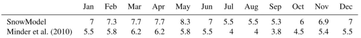
Air temperature proved to be a challenging parameter to calibrate due to the complex terrain of the MRB. Here, true temperature lapse rates do not always follow a linear temperature-elevation relationship and synoptic scale atmo-spheric patterns can affect local lapse rates, especially when high pressure systems dominate causing cold air pooling (Daly et al., 2010). For the model, we used initial monthly lapse rates from the Washington Cascades, roughly 350 km north of the MRB (Minder et al., 2010). These lapse rates were iteratively adjusted to minimize RMSE for temperature using the forcing and evaluation stations listed in Table 1. The final model iteration applied monthly lapse rate values ranging from 5.5–7◦C km−1 and were 1.5◦C km−1 cooler than Minder found in the Washington Cascades (Table 3). Minimum RMSE for some calibration sites were outside of the target threshold of 2◦C, as large errors for a few values can exacerbate RMSE values (Freedman et al., 1991). Thus R2values (Legates and McCabe, 1999) and 95 % confidence intervals were calculated (Freedman et al., 1991) to augment model evaluation.R2values describe the proportion (0.0 to 1.0) of how much of the observed data can be described by the model, and confidence intervals indicate simulation relia-bility. Methods on how to potentially improve lapse rate cal-culations for future work are described in the third paragraph of the Discussion section.
Table 3.Lapse rate values (◦C km−1)used in SnowModel and those published by Minder et al. The values posted by Minder et al. (2010) are for the Washington Cascades, which are approximately 350 km north of the MRB.
Jan Feb Mar Apr May Jun Jul Aug Sep Oct Nov Dec
SnowModel 7 7.3 7.7 7.7 8.3 7 5.5 5.5 5.3 6 6.9 7
Minder et al. (2010) 5.5 5.8 6.2 6.2 5.8 5.5 4 4 3.8 4.5 5.4 5.5
approach does not provide a detailed measurement of SWE in a 100 m×100 m grid cell, and thus was used as a broad metric for assessing the magnitude of simulated SWE and the timing of accumulation and ablation. Logistically, this rapid assessment approach allowed samples at all five sites to be conducted in a single day. In addition, colleagues at the University of Idaho provided SWE measurements at two lo-cations in the basin on two dates in WY 2008 and 2009 (Link et al., 2010).
2.4 Remote sensing based calibration
The spatial extent of modeled snow cover was assessed us-ing satellite-derived maps of fractional snow-covered area (fSCA). The Landsat TM fractional snow covered area data were aggregated from 30 m data to the 100 m grid resolu-tion of SnowModel and converted to a binary grid where <15 % fSCA was classified as nosnow, and>15 % fSCA was classified as snow in the grid cell. The co-occurrence of modeled and measured snow cover was assessed using metrics of accuracy, precision, and recall as in Painter et al. (2009). Precision is the probability that a pixel identi-fied with snow indeed has snow.Recall, the metric that Dong and Peters-Lidard (2010) employed, is the probability of de-tection of a snow-covered pixel.Accuracyis the probability a pixel is correctly classified. For detailed explanations of these measures and their application to snow mapping, see Rittger (2012).
There were a limited number of valid images each win-ter because of cloud cover common in maritime climates and the 16 day repeat cycle of Landsat. For example, during WY 2009, only one image between the months of Novem-ber and April had a cloud cover less than 25 % in the MRB. However, each calibration year had at least one image with cloud cover less than 10 % that could be used to effectively assess the spatial accuracy of the model. While the day of year of Landsat acquisition varied across years, multiple im-ages were acquired during accumulation, peak, and ablation phases of SWE. The spatial agreement between fSCA and SnowModel results was evaluated for physiographic vari-ables including land cover class, elevation, slope and aspect. This allows us to identify the physical characteristics of the domain that were potentially misrepresented by the model.
2.5 Climate perturbations
The calibrated and validated model was run for the study pe-riod and then used to assess the sensitivity of snowpack to increased temperature and variable precipitation. To deter-mine the response of snowpack to increased temperature and changes in precipitation, a sensitivity analysis was conducted in three phases. The first phase increased all temperature in-puts for WY 1989–2009 by 2◦C (hereafter referred to byT2), which is considered to be the mean annual average tempera-ture increase in the region by mid-century (Mote and Salath´e, 2010). The second and third phases retained the temperature increases, but also scaled precipitation inputs by±10 % to incorporate the uncertainty in projected future precipitation (Mote and Salath´e, 2010). Hereafter these phases will be re-ferred to byT2P10(representing+2◦C and a 10 % increase in precipitation), andT2N10(representing+2◦C and a 10 % decrease in precipitation). Results from the±10 % precipita-tion also provide insight into how annual variability in pre-cipitation can affect SWE relative to the effects of increased temperature. The model was then run, applying the three sets of scaled meteorological data for the study period of WY 1989–2009.
3 Results
3.1 Model assessment
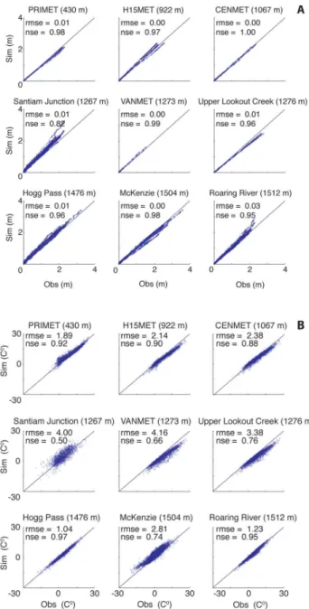
Model results were evaluated at SNOTEL stations, meteoro-logical stations in the HJA, and our field measurement sites (Figs. 2–4, Table 4). Model simulations ofP andTair
per-formed well at input stations (used to force the model) and reference stations (used to validate the model) (Fig. 2a and b). For years other than calibration and validation years, the mean NSE of P andTair at all stations was 0.97 and 0.80,
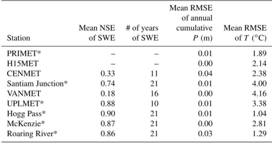
respectively (Table 4) during the snow season (1 November– 30 June). The model simulations of SWE (Figs. 3 and 4) showed mean NSE coefficients of 0.83 across the basin at automated SNOTEL locations and 0.70 at the field sites. Spa-tially, simulations had an overall accuracy of 82 % compared to the Landsat fSCA data.
Table 4.Mean Nash Sutcliffe Efficiency (NSE) Rating and Root Mean Squared Error for Daily SWE, andT and AnnualP. These stations all have 10 or years of record.
Mean RMSE of annual
Mean NSE # of years cumulative Mean RMSE
Station of SWE of SWE P (m) ofT (◦C)
PRIMET* – – 0.01 1.89
H15MET – – 0.00 2.14
CENMET 0.33 11 0.04 2.38
Santiam Junction* 0.74 21 0.01 4.00
VANMET 0.18 16 0.00 4.16
UPLMET* 0.88 10 0.01 3.38
Hogg Pass* 0.90 21 0.01 1.04
McKenzie* 0.87 21 0.00 2.81
Roaring River* 0.86 21 0.03 1.29
Stations noted by an asterisk * are SWE measurements that have been reviewed and calibrated.
showed that in a few cases there were significant discrepan-cies (>1 m of annual cumulative precipitation) at several of the stations that were used as forcing data. Additionally, a few large precipitation inputs were offset by one day. The shifts were not systematic and appeared to be random in na-ture, most likely due to equipment mistiming at several sta-tions. As a result storms with a significant amount of to-tal precipitation (>50 mm) were, in effect, double counted and processed on two consecutive days by the model. While the errors were present in less than 10 % of the datasets these events were characterized by heavy precipitation and cold temperatures that increased snowpack accumulation. This double count of precipitation provided simulations with around a 1 m overestimation of SWE, roughly the same mag-nitude as the over estimation of annual precipitation. Thus this year was omitted. WY 2005 displayed model deficien-cies in resolving lapse rates associated with temperature in-versions. Simulations of spatially distributed gridded temper-ature in WY 2005 had an RMSE of 3.8◦C and NSE of 0.72, whereas the study period had values of 2.5◦C and 0.80, re-spectively. This was due to extended periods of high pres-sure, which resulted in cold air pooling and negative tem-perature lapse rates (Daly et al., 2010). Extensive snowmelt and near complete loss of upper elevation snowpack oc-curred in mid-to-late February (National Resource Conser-vation Service, personal communication, 2009; National Re-source Conservation Service, 2012) as unseasonably warm temperatures at higher elevations and unseasonably cool tem-peratures at lower elevations persisted for several weeks. The model deficiencies caused by such extensive temperature in-versions are addressed in the Discussion section.
Precipitation was effectively distributed for all stations and across the full range of elevations used in the validation (Fig. 2a). The mean RMSE error was 0.01 m and the mean NSE value was 0.96 for the full study period. It is important to note that the addition of the low elevation Eugene Airport
meteorological station (174 m) greatly improved model per-formance. This station provided meteorological input data at a low elevation and at the western edge of the model domain, which improved the spatial interpolation of precipitation.
Air temperature had a mean RMSE of 2.5◦C and mean NSE value of 0.80 (Fig. 2b and Table 4). Model simulations at the Santiam Junction SNOTEL station consistently under-performed in relation to all other stations. Santiam Junction is adjacent to a state highway, an Oregon Department of Trans-portation facility, and an airstrip which combined, make it more exposed to wind than the nearby natural forest setting found at the other stations. The station elevation also pro-vided a small bias, as simulations at middle elevation stations (800–1300 m) underestimatedTairon average by 2.0◦C. The
upper elevation stations (1300–1550 m) overestimated tem-perature on average by 0.25◦C. This bias reflects the to-pographic character of the MRB. The upper elevation sites are situated in the High Cascades geological province, where the topography has a more gradual slope averaging approx-imately 10◦. In the Western Cascades (up to 1300 m) geo-logical province, slopes are steeper averaging approximately 20◦, but are also frequently characterized by slopes up to 50◦. In the Western Cascades during periods of high pressure, it is common to have cold air drainage, where cooler, more dense air moves down a slope and pools in valleys creating cooler temperatures at lower elevations (Daly et al., 2010).
The RMSE for Tair (2.5◦C) was larger than anticipated,
however further analysis showed anR2of 0.85 and 98 % of allTairsimulations within a 95 % confidence interval. The
ad-ditional evaluation metrics support the likelihood that a small minority of poor model simulations forTairhad a significant
Fig. 2.Model performance for precipitation (top –(a)) and temper-ature (bottom –(b)) in years not used in calibration and validation. Each dot represents a day during 1 November–30 June.
resolve these issues are found in the third paragraph of the Discussion section.
The model simulations of SWE (Figs. 3 and 4) showed mean NSE coefficients of 0.83 across the basin at point-based locations. The data record for SWE is more limited than the records ofP andTair and only the four SNOTEL
sites (elev. 1267 to 1512 m) have measurements of SWE that span the full data record. These sites provide the primary ref-erence points for model evaluation (Figs. 3 and 4). Compar-isons of observed and simulated values showed an RMSE of 0.13 m at all sites used in the validation SNOTEL sites
Modeled
Measured + 20C
0 0.5 1.0
SWE (m)
0 0.5 1.0
0 1.0 2.0
Oct Dec Feb Apr Jun 0
1.0 2.0
SWE (m)
0
Oct Dec Feb Apr Jun
Oct Dec Feb Apr Jun 0
1.0 2.0
1.0 2.0 nse = 0.95
nse = NaN
nse = 0.98
nse = 0.63
nse = 0.84 nse = 0.97
CENMET Santiam Junction Upper Lookout Creek
Hogg Pass McKenzie Roaring River
WY 1991 - Below Average Snowpack
WY 1999 - Above Average Snowpack
WY 2002 - Average Snowpack
0 0.5 1.0
SWE (m)
0 0.5 1.0
0 1.0 2.0
Oct Dec Feb Apr Jun 0
1.0 2.0
SWE (m)
0
Oct Dec Feb Apr Jun
Oct Dec Feb Apr Jun 0
1.0 2.0
1.0 2.0
nse = NaN nse = 0.84 nse = NaN
nse = 0.94 nse = 0.87 nse = 0.94
CENMET Santiam Junction Upper Lookout Creek
Hogg Pass McKenzie Roaring River
0 0.5 1.0
SWE (m)
CENMET
0 0.5 1.0
Santiam Junction
0 1.0 2.0
Upper Lookout Creek
Oct Dec Feb Apr Jun 0
1.0 2.0
Hogg Pass
SWE (m)
0
Oct Dec Feb Apr Jun
Oct Dec Feb Apr Jun 0
1.0 2.0
McKenzie
1.0 2.0
Roaring River
nse = 0.67 nse = 0.86 nse = 0.92
nse = 0.99 nse = 0.99 nse = 0.90
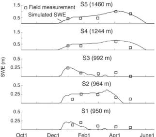
Fig. 4.Model performance of SWE at field locations in WY 2009. Location of field sites are shown in Fig. 1.
(Table 4). Field measurements collected at a range of eleva-tions during WY 2008 and 2009 also show a high level of agreement between measured and modeled SWE values with an NSE coefficient of 0.70 (Fig. 4). These field sites suggest that model results successfully simulate the timing and mag-nitude of snowpack evolution, especially at the higher eleva-tions. The lower elevation sites (S1–S3) show a lower level of agreement during the ablation period. Here, spring SWE is less than 0.1 m and the mean difference between the ob-served and simulated values during the ablation period was only 0.07 m. It is worth noting the highest SNOTEL site is situated at an elevation of 1512 m, but 75 % of the model-estimated SWE lies above that elevation. This result is con-sistent with the work of Gillan et al. (2010) who found that >70 % of SWE accumulates above the mean elevation sur-rounding SNOTEL sites in a snow-dominated watershed in Northwestern Montana.
The length and consistency of the automated SWE data record at lower elevation sites is more limited. With the ex-ception of UPL, snow pillows in the HJA are not calibrated and the reported data have not been fully quality assured. The result is an inconsistent dataset with values that often do not represent expected snowpack evolution in the region. Due to the questionable accuracy of the measured SWE values in the HJA, these data were not used as a metric for model valida-tion. This issue also highlights the need for a careful calibra-tion and regular maintenance of SWE measurement sites.
In the spatial validation, 14 yr of SnowModel simulations of snow cover compared to Landsat TM fSCA (converted to snow/no snow) had an overall accuracy of 82 % (the ratio of correctly identified grid cells – i.e. snow as snow, bare as bare), and overall precision of 71 % (the probability that a pixel identified with snow indeed has snow) and an overall recall of 93 % (the proportion of positives correctly
identi-fied as positives). Although the accuracy statistic may rise be-cause of overwhelming numbers of cells in which there is no snow (Rittger et al., 2012), we include it because a large por-tion of the MRB can be snow covered and validapor-tion scenes are distributed throughout the season. Disagreement between the fSCA images and simulations primarily occurred where the model estimated snow cover and the fSCA did not have snow cover (13 %). This degree of False Positive (FP) is ex-pected as remotely sensed data typically omits snow cover in the steep and heavily forested landscapes that dominate the Western Cascades and the MRB (Nolin, 2011). The inter-annual changes associated with harvested forest are not ex-pressed in the static land cover dataset, but are incorporated into the fSCA product. This classification discrepancy prop-agated through each year contributing to the lower precision value by decreasing the number of True Positive (TP). Ad-ditionally, the fSCA binary product classifies any cell with a fractional snow cover value less than 15 % asno snow. Even though the Landsat fSCA product was coarsened to 100 m, cells at the transitional snow line will be classified as no snow and result in an increase in False Positive (FP) classifications for modeled snow cover. WY 2006, 2008, and 2009 were the exceptions, showing more False Negative (FN) classifi-cations, but with a similarly higher level of agreement. For a more detailed discussion of the model assessment using remote-sensing data, please refer to Sproles (2012).
3.2 Impacts of warmer climate and changing precipitation on snow
Sensitivity of snowpack to changes in temperature and precipitation
Fig. 5.Map of simulated SWE on 1 April 2009 for Reference conditions.
Table 5.Changes in peak SWE, % of peak SWE lost, and the shift in the number of days earlier for the MRB averaged across the ref-erence period.
Mean Peak SWE (km3) 1.26
Mean Date of Peak SWE 31 March
Scenario
Mean Peak T2 0.56
SWE (km3) T2P10 0.64
T2N10 0.48
% of Mean Peak T2 56
SWE Lost T2P10 49
T2N10 62
Shift of Mean T2 12
Date of Peak T2P10 6
SWE (days) T2N10 22
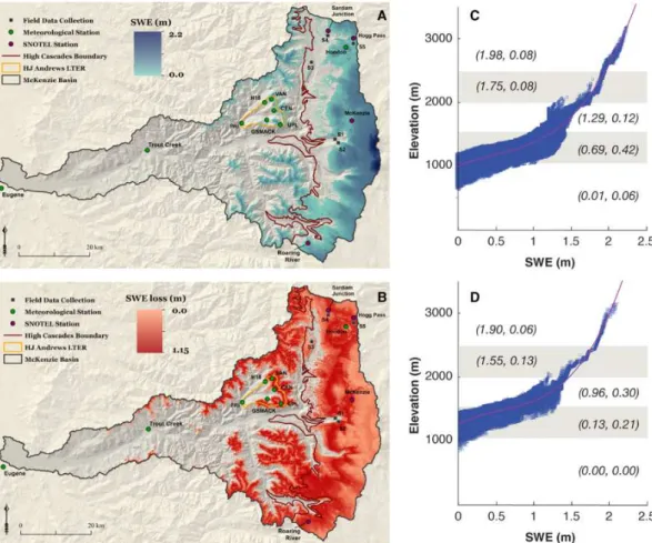
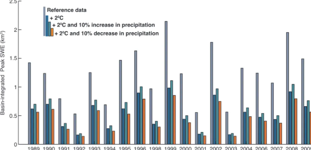
MRB. The 0.21 km3 (69 mm) difference of area-integrated peak SWE predicted by theT2P10andT2N10scenarios is substantial and is equal to slightly less than available storage at Cougar Reservoir. However, 2◦C temperature increases alone result in a 0.70 km3loss (230 mm of SWE distributed across the basin, Figs. 6a–d and 7, Table 5). Increased pre-cipitation in theT2P10scenario results in additional SWE at elevations primarily over 1800 m, where a 2◦C increase in temperature is not sufficient to convert snowfall to rainfall or to significantly accelerate snowmelt. However, this increase in SWE at the high elevations only partially offsets some of the losses at lower elevations.
With warmer conditions, the date of peak SWE is pro-jected to occur earlier in the spring and properly into the winter (before the vernal equinox). The average date for sim-ulated peak SWE in the MRB during the study period is 31 March. However, inT2the average date for peak SWE shifts 12 days earlier in the WY. Similarly, peak SWE arrives 6 days and 22 days earlier in theT2P10andT2N10 scenar-ios, respectively, indicating a greater sensitivity in theT2N10 than theT2P10scenario.
We assessed the sensitivity of the snowpack to tempera-ture increases by elevation using the 10 day mean of peak SWE and frequency of snow cover for WY 2007. The 10 day mean of peak SWE minimized the influence of any single large accumulation event in order to emphasize the overall snowpack trend for that season. WY 2007 was a statistically average year for SWE at the four SNOTEL sites. Peak SWE was−0.07 m of the reference mean and had a standard de-viation of 0.02 m from the reference mean value (0.83 m). In WY 2007 the greatest net losses of peak SWE were found be-tween 1001 and 1500 m (Fig. 8). This elevation zone gener-ated 53 % of the basin-wide losses of SWE in theT2scenario, and comprises 45 % of the basin area. Proportionately, the areas between 1501 and 2000 m generate a more significant component of peak SWE loss. This elevation zone generated 45 % of the basin-wide peak SWE losses in theT2scenario, but comprises only 17 % of the basin area. The mean loss of peak SWE lost per grid cell was 0.61 m in this elevation zone, as compared to 0.26 m in areas between 1001 and 1500 m.
Fig. 6.Map of simulated SWE on 1 April 2009 with a 2◦C increase in temperature(a). Map of the loss of simulated SWE on 1 April 2009 with a 2◦C increase in temperature(b). SWE by elevation on 1 April 2009 using reference observed data(c). SWE by elevation on 1 April 2009, 2009 with a 2◦C increase in temperature(d). Each dot on the plot represents a grid cell in the MRB. The values in parentheses represent the mean SWE and standard deviation of SWE(meanSWE, stdSWE)at each elevation band. The upper elevations are not affected as significantly as the lower elevation snowpack.
the basin, with the areas between 1001 and 1500 m affected the most. This range of elevations saw an average of 36 fewer days of snow cover than in the reference year (Fig. 8). Ele-vations between∼1501 and 2000 m see a less dramatic re-duction of snow covered days. Areas between∼2001 and 2500 m experienced increased losses in snow cover days with elevation.
4 Discussion
Our results quantified the basin-wide distribution and volu-metric storage of snow water in the MRB, which averaged 1.26 km3of SWE (414 mm distributed across the basin) over the study period. This natural “reservoir” stores roughly five times more water than the largest impoundment in the water-shed. The maritime snowpack of the MRB was highly sensi-tive to increased temperatures, showing a 56 % loss in peak SWE when temperature forcings were increased by 2◦C. Projected warmer conditions also hasten the melt cycle, with
peak SWE occurring 12 days earlier. Elevations between 1000 and 2000 m are most affected in theT2scenario as snow transitions to rain, and snow on the ground has an enhanced melt cycle (Fig. 3). Figure 6c–d suggest that a 2◦C temper-ature increase will shift snowpack characteristics by approx-imately 250 m. The elevation zone from 1000–1500 m has the greatest volumetric loss of stored water (Figs. 6a–d and 8), and represents the largest areal proportion of the basin. In WY 2009, mean SWE values for this elevation band diminish considerably, from 0.69 to 0.13 m. Elevations above 2000 m are affected by warmer temperatures, but to a lesser extent, retaining a similar average SWE by elevation (Fig. 6c–d).
1989 1990 1991 1992 1993 1994 1995 1996 1998 1999 2000 2001 2002 2003 2004 2006 2007 2008 2009 0
0.5 1 1.5 2 2.5
Basin-wide SWE Sensitivity
Basin-integrated Peak SWE (km
3)
+ 20C
+ 20C and 10% increase in precipitation
+ 20C and 10% decrease in precipitation
Reference data
Fig. 7.Peak SWE integrated over the area of the MRB and its sensitivity to a 2◦C increase in temperature.
increases in theT2P10scenario above∼2000 m where in-creased precipitation also increases the seasonal accumula-tion of SWE. However even with gains at high elevaaccumula-tions, there is still a considerable net loss of snowpack (−49 %) compared to the study period. Not surprisingly, the response of snow cover frequency to a 2◦C increase is very similar to the pattern of the change in SWE (Fig. 8). Snow cover duration in the elevation zone from 1000–1500 m were most affected, with some locations losing more than 80 days of snow cover in an average snow year.
Initially the meandering nature of the snow loss curves in Fig. 8 might not seem intuitive, but can be explained by the topography of the MRB. Elevations between∼1001 and 1500 m can receive both rain and snow during the winter, even though elevations above 1200 m retain a seasonal snow-pack. This elevation range is the most sensitive to increased temperature and shows a transition to a rain-dominated area with a 2◦C increase. Elevations between∼1501 and 2000 m are less sensitive to increased temperatures and more likely to retain enough precipitation falling as snow with a 2◦C in-crease to develop distinct periods of accumulation and ab-lation. Retention of the snowpack in this elevation range is aided by the highly-dissected Western Cascades (which dom-inate this elevation) where adjacent terrain provides shade, reduces incoming short-wave radiation, and mitigates poten-tial snow loss (DeWalle and Rango, 2008). This shading also helps explain the loss of snow between∼2000 and 2500 m, where topography shifts from the rugged Western Cascades to the more exposed High Cascades. This shift towards a gradual, consistent slope in the High Cascades provides less shading throughout the course of day that would potentially mitigate increased temperatures.
Efforts in calibrating and validating the model clearly demonstrated that precipitation and temperature are first or-der controls on snowpack accumulation and peak SWE. This highlights that it is critical to achieve optimal accuracy of the
spatially distributed values ofP andTairprior to calibrating
the model based on SWE.P had a high level of agreement between observations and simulations (NSE of 0.97). There were distinct similarities between theR2(0.85) and NSE of Tair (0.80) with the NSE of SWE (0.83) and the accuracy
of the spatial distribution of snowpack (82 %). These simi-larities lead to the logical conclusion that improvements in accuracy of snowpack simulations can be made through im-provements in temperature simulations.
The challenges in simulatingTairare partially explained by
the physical characteristics of the MRB. Daly et al. (2010) used empirical data to establish that expected temperature lapse rates that exist between elevation and temperature are often decoupled from one another and are largely controlled by topography and elevation. Steeper slopes can produce cold air drainage and different lapse rates than lapse rates for more gentle slopes (Daly et al., 2010). Additionally, moisture content of a storm (as determined by its temperature, source area, and history) affects the wet adiabatic lapse rate. Daly et al. (2010) suggest that variability in lapse rates may in-crease with projected future climate. Combined, these factors highlight the shortcomings of using a standard temperature lapse rate in a model. Though outside of the scope of this re-search, an improvement to the monthly static lapse rates used in SnowModel would be to compute dynamic lapse rates with a dual-pass approach. The first pass through the meteorolog-ical station data would establish the lapse rate and the second pass would apply time step specific lapse rates in the Barnes Objective Analysis method to spatially distribute tempera-ture data. This would allow an individual storm’s lapse rate characteristics to be included in the model. A dynamic lapse rate would also help during stable conditions when cold air drainage may be important.
Fig. 8.Loss of SWE (upper) and snow covered days (lower) by elevation with a 2◦C increase on 1 April 2007. Each dor on the plot represents a grid cell in the MRB. Snowpack between 1000 and 2000 m are the most sensitive to temperature and show the greatest losses.
stations in the HJA decreased overall model accuracy by skewing the data spacing in the weighting scheme. To cre-ate a balanced simulation ofTairandP requires stations that
are widely spaced and that span the range of elevation values. Iterative testing of the model with various station combina-tions revealed that it was best to use just two stacombina-tions in the HJA in the final model implementation: PRI (elev. 430 m) and UPL (elev. 1294 m). The addition of the Eugene station (elev. 174 m) also improved model agreement by providing a datum in the western portion of the basin. Incorporating the meteorological data from Hogg Pass, McKenzie, and Roar-ing River created anchor points in the eastern portion of the basin. These locations were especially pertinent in address-ing the challenges associated with distributaddress-ing temperature across the basin.
While this study achieved a high level of agreement be-tween simulated and measured values, the complex topog-raphy and land cover of the MRB also introduce potential sources of error. While the MicroMet and EnBal sub-models implicitly included land cover and topography in calculat-ing incomcalculat-ing shortwave radiation, the albedo function did not account for these factors in reflected shortwave radia-tion. An improved albedo function inclusive of land cover and topography would provide the opportunity to reduce or account for model error. Similarly, there are limitations in estimating snow cover extent in complex terrain using re-motely sensed images (Rittger et al., 2013). The thick vege-tation of the MRB potentially obscures snow underneath the
forest canopy. Our validation applied the most recent scien-tific advances in calculating fSCA in mountainous regions (Rittger et al., 2013), that can be improved in future work by field validation.
The elevation range of stations (174–1512 m) limited model assessment at higher elevations. Hypsometrically, this comprises 74 % of the basin, and extends from regions domi-nated by rain into the seasonal snow zone above 1200 m. The authors recognize that higher elevation measurements would have benefitted the study, and could help minimize uncer-tainty in future research. Unfortunately access to elevations above 2000 m was not logistically feasible during the field season. Future improvements in field methods would include at least one high elevation site above 1800 m rather than three lower elevation sites. Data was also limited temporally, with hourly data beginning in WY 1999. Because one of the pri-mary goals of the study was to simulate snowpack for multi-ple decades, we moved forward pragmatically, applying the best data available supplemented by field observations. We are applying our findings to improve field measurements in the basin that will ultimately aid future model-based studies in this watershed and region.
Looking forward – the impacts of climate perturbations on snowpack
Losses in SWE and declining snow duration will impact years with high, low and average snowpack and will change the statistical representation and human perceptions of what a high, low and average snowpack represents. The MRB will increasingly experience more precipitation falling as rain rather than snow in warmer conditions. Areas presently in the rain/snow transition zone will become dominated almost en-tirely by rain. The changes will affect the timing and magni-tude of runoff during the winter, spring, and summer months as more precipitation shifts from snow to rains (Stewart et al., 2005; Jefferson et al., 2008; Jefferson, 2011).
the year, dam operations will need to reflect these changes in their management strategy. Results from this study have already helped water resource professionals choose a site for a new SNOTEL station to augment the existing monitor-ing network (Webb, personal communication, 2011) and de-velop water management strategies for municipal water use (Morgenstern, personal communication, 2010).
Snow and snowmelt serve as a resource for winter and summer recreation, agriculture, industry, municipalities, and hydropower. The difference with a 2◦C increase in tempera-ture on peak area-integrated SWE is considerable (0.70 km3 or 230 mm of basin-wide SWE) – more than twice the size of the largest impoundment in the basin. While this esti-mated loss only pertains to the MRB it would scale up to be major factor at the regional level. Potential management concerns pertaining to the supply of water could be com-pounded by shifts in the demand of water as well. Oregon’s population is expected to grow by 400 000 from 2010 to 2020 (Office of Economic Analysis, 2011). The increase in population would most likely increase demand especially in the summer and fall when stakeholders compete for an al-ready limited supply (United States Army Corps of Engi-neers, 2001; Oregon Water Supply and Conservation Initia-tive, 2008). Because mountain snowpack serves as an effi-cient and cost-effective reservoir, any research that examines socio-economic topics should contain a mountain snowpack component. For example, an examination of socio-economic impacts of the adaption costs associated with mitigating cli-mate change would need to include the costs associated with a diminished mountain snowpack.
5 Conclusions
This research provided the first detailed spatial and tempo-ral understanding of snow accumulation and ablation in the MRB for present conditions and serves as a prognostic tool for understanding snowpack in projected future climates. Be-cause maritime snow accumulates at temperatures close to 0◦C, the seasonal accumulation and ablation of maritime snow is sensitive to temperature. These findings provide in-sights into the mechanisms controlling snowpacks in such environments and serves as an example of the magnitude and types of changes that may affect similar watersheds in a warmer climate. Moreover, with the modifications made to the model (rain-snow partitioning, albedo decay function), this model can readily be transitioned to other regions with maritime snow with minimal reconfiguration. Although this study focused on a single watershed, the processes affecting snowpack in the McKenzie River are similar to other mar-itime snowpacks across the Earth.
Mountain snowpack is a key common-pool resource, pro-viding a natural reservoir that supplies water for drinking, worship, hydropower, agriculture, ecosystems, industry, and recreation for over 1 billion people globally. The spatial
dis-tribution of maritime snowpack and its sensitivity to cli-mate change at basin scale does not provide global answers, but it does provide clarity at a scale appropriate for de-veloping management strategies for the future (Seibert and McDonnell, 2002).
Acknowledgements. This research was supported by National Science Foundation grant #0903118 and through initial funding provided by the Institute for Water and Watersheds at Oregon State University. The authors would like to thank Jeff McDonnell, Christina Tague, John Bolte, Bettina Schaefli (editor), and the reviewers for their contributions that helped improve the quality of this manuscript.
Edited by: B. Schaefli
References
Abatzoglou, J. T.: Influence of the PNA on declining mountain snowpack in the Western United States, Int. J. Climatol., 31, 1135–1142, doi:10.1002/joc.2137, 2011.
Andersen, M. G. and Bates, P. D.: Hydrological Science: Model Credibility and Scientific Integrity, in: Model validation: per-spectives in hydrological science, edited by: Andersen, M. G. and Bates, P. D., J. Wiley, Chichester, New York, xi, 500 p., 2001. Armstrong, J. S. and Collopy, F.: Error measures for generalizing
about forecasting methods: Empirical comparisons, Int. J. Fore-cast., 8, 69–80, 1992.
Bales, R. C., Molotch, N. P., Painter, T. H., Dettinger, M. D., Rice, R., and Dozier, J.: Mountain hydrology of the western United States, Water Resour. Res., 42, W08432, doi:10.1029/2005wr004387, 2006.
Barnett, T. P., Adam, J. C., and Lettenmaier, D. P.: Potential impacts of a warming climate on water availability in snow-dominated regions, Nature, 438, 303–309, doi:10.1038/nature04141, 2005. Bavay, M., Lehning, M., Jonas, T., and L¨owe, H.: Simulations of
fu-ture snow cover and discharge in Alpine headwater catchments, Hydrolog. Process., 23, 95–108, 2009.
Brooks, J. R., Wigington, P. J., Phillips, D. L., Comeleo, R., and Coulombe, R.: Willamette River Basin surface water isoscape (δ18O andδ2H): temporal changes of source water within the river, Ecosphere, 3, 39, doi:10.1890/es11-00338.1, 2012. Brown, A.: Understanding the Impact of Climate Change on
Snow-pack Extent and Measurement in the Columbia River basin and Nested Sub Basins, Masters of Science, Geosciences, Oregon State University, 2009.
Brown, D. P. and Kipfmueller, K. F.: Pacific Climate Forcing of Multidecadal Springtime Minimum Temperature Variability in the Western United States, Ann. Assoc. Am. Geogr., 102, 521– 530, doi:10.1080/00045608.2011.627052, 2012.
Burles, K. and Boon, S.: Snowmelt energy balance in a burned for-est plot, Crowsnfor-est Pass, Alberta, Canada, Hydrolog. Process., 25, 3012–3029, doi:10.1002/hyp.8067, 2011.
DeWalle, D. R. and Rango, A.: Principles of snow hydrology, Cam-bridge University Press, CamCam-bridge, UK, 410 pp., 2008. Dong, J. and Peters-Lidard, C.: On the relationship between
tem-perature and MODIS snow cover retrieval errors in the Western US, Selected Topics in Applied Earth Observations and Remote Sensing, IEEE J. Sel. Top. Appl., 3, 132–140, 2010.
Dozier, J.: Mountain hydrology, snow color, and the
fourth paradigm, Eos Trans. AGU, 92, 373–375,
doi:10.1029/2011eo430001, 2011.
Freedman, D., Pisani, R., Purves, R., and Adhikari, A.: Statistics, 2nd Edn., WW Norton and Company, New York, 514 pp., 1991. Fritze, H., Stewart, I. T., and Pebesma, E.: Shifts in West-ern North American Snowmelt Runoff Regimes for the Recent Warm Decades, J. Hydrometeorol., 12, 989–1006, doi:10.1175/2011jhm1360.1, 2011.
Fry, J. A., Coan, M. J., Homer, C. G., Meyer, D. K., and Wickham, J. D.: Completion of the National Land Cover Database (NLCD) 1992–2001 Land Cover Change Retrofit product: US Geological Survey Open-File Report, 2008, US Geological Survey, 18, 2009. Gesch, D. B.: The National Elevation Dataset, in: Digital Elevation Model Technologies and Applications: The DEM Users Man-ual, edited by: Maune, D., American Society for Photogramme-try and Remote Sensing, Bethesda, Maryland, 99–118, 2007. Gillan, B. J., Harper, J. T., and Moore, J. N.: Timing of present
and future snowmelt from high elevations in northwest Montana, Water Resour. Res., 46, W01507, doi:10.1029/2009wr007861, 2010.
Hulse, D., Gregory, S., and Baker, J. P.: Willamette River Basin planning atlas: trajectories of environmental and ecological change, Oregon State University Press, Corvallis, OR, 2002. Iziomon, M. G., Mayer, H., and Matzarakis, A.: Downward
atmo-spheric longwave irradiance under clear and cloudy skies: Mea-surement and parameterization, J. Atmos. Solar-Terrest. Phys., 65, 1107–1116, 2003.
Jefferson, A. J.: Seasonal versus transient snow and the elevation de-pendence of climate sensitivity in maritime mountainous regions, Geophys. Res. Lett., 38, L16402, doi:10.1029/2011gl048346, 2011.
Jefferson, A., Nolin, A., Lewis, S., and Tague, C.: Hydrogeologic controls on streamflow sensitivity to climate variation, Hydrolog. Process., 22, 4371–4385, doi:10.1002/hyp.7041, 2008.
Kirchner, J. W.: Getting the right answers for the right rea-sons: Linking measurements, analyses, and models to advance the science of hydrology, Water Resour. Res., 42, W03S04, doi:10.1029/2005wr004362, 2006.
Knowles, N., Dettinger, M. D., and Cayan, D. R.: Trends in Snow-fall versus RainSnow-fall in the Western United States, J. Climate, 19, 4545–4559, 2006.
Koch, S. E., desJardins, M., and Kocin, P. J.: An Interactive Barnes Objective Map Analysis Scheme for Use with Satellite and Conventional Data, J. Clim. Appl. Meteorol., 22, 1487–1503, doi:10.1175/1520-0450(1983)022, 1983.
Legates, D. R. and McCabe, G. J.: Evaluating the use of “goodness-of-fit” measures in hydrologic and hydroclimatic model valida-tion, Water Resour. Res., 35, 233–241, 1999.
Lehning, M., V¨olksch, I., Gustafsson, D., Nguyen, T. A., St¨ahli, M., and Zappa, M.: ALPINE3D: a detailed model of mountain sur-face processes and its application to snow hydrology, Hydrolog. Process., 20, 2111–2128, doi:10.1002/hyp.6204, 2006.
Link, T., Snyder, A., Metzger, S., and Hacking, J.: SWE Mea-surements for the McKenzie River Basin, University of Idaho, Moscow, ID, 2010.
Liston, G. E. and Elder, K.: A Meteorological Distribution System for High-Resolution Terrestrial Modeling (MicroMet), J. Hy-drometeorol,, 7, 217–234, 2006a.
Liston, G. E. and Elder, K.: A Distributed Snow-Evolution Mod-eling System (SnowModel), J, Hydrometeorol,, 7, 1259–1276, 2006b.
Liston, G. E., Haehnel, R. B., Sturm, M., Hiemstra, C. A., Bere-zovskaya, S., and Tabler, R. D.: Instruments and Methods Simu-lating complex snow distributions in windy environments using SnowTran-3D, J, Glaciol,, 53, 241–256, 2007.
Luce, C. H. and Holden, Z. A.: Declining annual streamflow distri-butions in the Pacific Northwest United States, 1948–2006, Geo-phys. Res. Lett., 36, L16401, doi:10.1029/2009gl039407, 2009. Marks, D., Domingo, J., Susong, D., Link, T., and Garen, D.: A
spatially distributed energy balance snowmelt model for appli-cation in mountain basins, Hydrolog. Process., 13, 1935–1959, doi:10.1002/(sici)1099-1085(199909)13:12/13< 1935::aid-hyp868>3.0.co;2-c, 1999.
Minder, J. R., Mote, P. W., and Lundquist, J. D.: Surface temperature lapse rates over complex terrain: Lessons from the Cascade Mountains, J. Geophys. Res., 115, D14122, doi:10.1029/2009jd013493, 2010.
Molotch, N. P. and Bales, R. C.: SNOTEL representativeness in the Rio Grande headwaters on the basis of physiographics and remotely sensed snow cover persistence, Hydrol. Process., 20, 723–739, 2006.
Molotch, N. P., Painter, T. H., Bales, R. C., and Dozier, J.: Incorporating remotely-sensed snow albedo into a spatially-distributed snowmelt model, Geophys. Res. Lett., 31, L03501, doi:10.1029/2003gl019063, 2004.
Moriasi, D. N., Arnold, J. G., Van Liew, M. W., Bingner, R. L., Harmel, R. D., and Veith, T. L.: Model Evaluation Guidelines for Systematic Quantification of Accuracy in Watershed Simula-tions, Trans. AASBE, 50, 885–900, 2007.
Mote, P. W.: Climate-Driven Variability and Trends in Mountain Snowpack in Western North America, J. Climate, 19, 6209– 6220, 2006.
Mote, P. and Salath´e, E.: Future climate in the Pacific North-west, Clim. Change, 102, 29–50, doi:10.1007/s10584-010-9848-z, 2010.
Mote, P. W., Hamlet, A. F., Clark, M. P., and Lettenmaier, D. P.: De-clining Mountain Snowpack in Western North America, B. Am. Meteorol. Soc., 86, 39–49, 2005.
Nash, J. E. and Sutcliffe, J. V.: River flow forecasting through con-ceptual models part I – A discussion of principles, J. Hydrol., 10, 282–290, 1970.
National Resource Conservation Service: NRCS SNOTEL data, United States Department of Agriculture, available at: http:// www.wcc.nrcs.usda.gov/snotel/Oregon/oregon.html, last access: 30 November, 2012.
National Resource Conservation Service: NRCS SNOTEL data, United States Department of Agriculture, available at: http: //www.wcc.nrcs.usda.gov/nwcc/sitenotes?sitenum=619, last ac-cess: 1 April, 2013.
Nolin, A. W.: Perspectives on Climate Change, Mountain Hydrol-ogy, and Water Resources in the Oregon Cascades, USA, Moun-tain Res. Develop., 32, S35–S46, doi:10.1659/mrd-journal-d-11-00038.s1, 2012.
Nolin, A. W. and Daly, C.: Mapping “At Risk” Snow in the Pacific Northwest, J. Hydrometeorol., 7, 1164–1171, 2006.
Nolin, A. W., Sproles, E. A., and Brown, A.: Climate change im-pacts on snow and water resources in the Columbia, Willamette, and McKenzie River Basins, USA: A nested watershed study, in: Transboundary River Governance in the Face of Uncertainty: The Columbia River Treaty, edited by: Cosens, B., Oregon State University Press, Corvallis, OR, 2012.
Office of Economic Analysis: Oregon’s Demographic Trends, State of Oregon, Salem, Oregon, 2011.
Oregon Water Supply and Conservation Initiative: Southern Willamette Valley Municipal Water Providers Final Report, 64, 2008.
Pagano, T., Garen, D., and Sorooshian, S.: Evaluation of official western US seasonal water supply outlooks, 1922–2002, J. Hy-drometeorol., 5, 896–909, doi:10.1175/1525-7541(2004), 2004. Painter, T. H., Rittger, K., McKenzie, C., Slaughter, P., Davis, R.
E., and Dozier, J.: Retrieval of subpixel snow covered area, grain size, and albedo from MODIS, Remote Sens. Environ., 113, 868– 879, 2009.
Rittger, K.: Spatial estimates of snow water equivalent in the Sierra Nevada PhD, The Bren School of Environmental Science and Management, University of California, Santa Barbara, University of California, Santa Barbara, 2012.
Rittger, K., Painter, T. H., and Dozier, J.: Assessment of methods for mapping snow cover from MODIS, Adv. Water Resour., 51, 367–380, doi:10.1016/j.advwatres.2012.03.002, 2013.
Rosenthal, W. and Dozier, J.: Automated Mapping of Mon-tane Snow Cover at Subpixel Resolution from the Land-sat Thematic Mapper, Water Resour. Res., 32, 115–130, doi:10.1029/95wr02718, 1996.
Seibert, J. and McDonnell, J. J.: On the dialog between experimen-talist and modeler in catchment hydrology: Use of soft data for multicriteria model calibration, Water Resour. Res., 38, 1241, doi:10.1029/2001wr000978, 2002.
Serreze, M. C., Clark, M. P., Armstrong, R. L., McGinnis, D. A., and Pulwarty, R. S.: Characteristics of the western United States snowpack from snowpack telemetry (SNOTEL) data, Water Re-sour. Res., 35, 2145–2160, 1999.
Service, R. F.: As the West Goes Dry, Science, 303, 1124–1127, 2004.
Sproles, E. A.: Climate change impacts on mountain snowpack presented in a knowledge to action framework PhD, Water Re-sources Graduate Program, Oregon State University, Oregon State University, 2012.
Stewart, I. T.: Changes in snowpack and snowmelt runoff for key mountain regions, Hydrolog. Process., 23, 78–94, doi:10.1002/hyp.7128, 2009.
Stewart, I. T., Cayan, D. R., and Dettinger, M. D.: Changes in Snowmelt Runoff Timing in Western North America under a “Business as Usual” Climate Change Scenario, Clim. Change, 62, 217–232, 2004.
Stewart, I. T., Cayan, D. R., and Dettinger, M. D.: Changes toward earlier streamflow timing across western North America, J. Cli-mate, 18, 1136–1155, 2005.
Strack, J. E., Liston, G. E., and Pielke Sr, R. A.: Modeling snow depth for improved simulation of snow-vegetation-atmosphere interactions, J. Hydrometeorol., 5, 723–734, 2004.
Sturm, M., Holmgren, J., and Liston, G. E.: A Seasonal Snow Cover Classification System for Local to Global Applications, J. Cli-mate, 8, 1261–1283, 1995.
Tague, C. and Grant, G. E.: A geological framework for inter-preting the low-flow regimes of Cascade streams, Willamette River Basin, Oregon, Water Resour. Res., 40, W04303, doi:10.1029/2003wr002629, 2004.
Tague, C., Grant, G., Farrell, M., Choate, J., and Jefferson, A.: Deep groundwater mediates streamflow response to climate warming in the Oregon Cascades, Clim. Change, 86, 189–210, doi:10.1002/hyp.8067, 2008.
United States Army Corps of Engineers: Comprehensive Water Supply Study – An examination of current water supply issues, Alexandria, Virginia, 2001.