Generalised cascades
S´ılvio M. Duarte Queir´os Unilever R&D Port Sunlight Quarry Road East, CH63 3JW, UK
(Received on 19 December, 2008)
In this manuscript we give thought to the aftermath on the stable probability density function when standard multiplicative cascades are generalised cascades based on theq-product of Borges that emerged in the context of non-extensive statistical mechanics.
Keywords:q-product, Nonextensivity, Log-normal distribution
1. INTRODUCTION
In the twenty years that have elapsed since the publication of the non-additive entropy Sq, which is also fairly known as Tsallis entropy [1], many applications and connections with to natural and man-mind phenomena have been estab-lished [2]. One of the most exciting applications which have emerged within the non-extensive scope is the definition of a whole new set of mathematical operations/functions that goes from the generalised algebra independently defined by Borges [3] and Nivanenet al. [4] and the integro-differential opera-tors by Borges to theq-trigonometric functions [5]. Besides its inherent beauty, these generalisations have found its own field of applicability. Namely, theq-product plays a primary role in the definition of theq-Fourier transform [6], thus inq -Central Limit Theorem [7], whereas the generalised trigono-metric functions have been quite successful in describing the critical behaviour of a class of composed materials known as manganites [8]. In this article, we inquire into the possi-ble applications of theq-product in the generation of random variables and its consequence on the definition of a new class of probability density functions.
2. PRELIMINARIES: THEq-PRODUCT
Theq-product,⊗q, has been introduced with the purpose to find a functional form that is able to generalise, in a non-extensive way, the mathematical identity,
exp[lnx+lny] =x×y, (x,y>0), (1) so that the equality,
x⊗qy≡expq[lnqx+lnqy], (2) holds. The representations lnq(.)and expq(.)correspond to theq-logarithm [9],
lnq(x)≡
x1−q−1
1−q , (x>0,q∈ℜ), (3)
and its inverse, theq-exponential,
expq(x)≡[1+ (1−q)x]1−1q, (x,q∈ℜ), (4)
respectively (expq(x) =0 if 1+ (1−q)x≤0). Forq→1, equation (2) recovers the usual property,
ln(x×y) =lnx+lny
(x,y>0), withx×y≡x⊗1y. Its inverse operation, theq -division,x⊘qy, verifies the following equality(x⊗qy)⊘qy= x.
Bearing in mind that the q-exponential is a non-negative function, theq-product must be restricted to the values ofx andythat respect the condition,
|x|1−q+|y|1−q−1≥0. (5) Moreover, we can extend the domain of theq-product to neg-ative values ofxandywriting it as,
x⊗qy≡ sign(x y)expq[lnq|x|+lnq|y|]. (6) Regarding some key properties of theq-product we mention:
1. x⊗1y=x y; 2. x⊗qy=y⊗qx;
3. (x⊗qy)⊗qz=x⊗q(y⊗qz) =x1−q+y1−q−2 1 1−q;
4. (x⊗q1) =x;
5. lnq[x⊗qy]≡lnqx+lnqy;
6. lnq(x y) =lnq(x) +lnq(y) + (1−q)lnq(x)lnq(y); 7. (x⊗qy)−1=x−1⊗2−qy−1;
8. (x⊗q0) =
0 if (q≥1 andx≥0) or if(q<1 and 0≤x≤1)
x1−q−1
1
1−q otherwise
|x|1−q+|y|1−q−1<0 is verified. According to the cut-off of theq-exponential, a value of zero forx⊗qyis set down in these cases. Restraining our analysis of Eq. (5) to the sub-spacex,y>0, we can observe that forq→ −∞the re-gion{0≤x≤1,0≤y≤1}is not defined. As the value ofq increases, the forbidden region decreases its area, and when q=0, we have the limiting line given byx+y=1, for which x⊗0y=0. Only forq=1, the entire set ofxandyreal values has a defined value for theq-product. Forq>1, the condi-tion (5) implies a region, |x|1−q+|y|1−q=1 for which the q-product diverges. This undefined region augments its area asqgoes to infinity. Whenq=∞, theq-product is only de-fined in{x≥0,0≤y≤1} ∪ {0≤x≤1,y>1}. Illustrative plots are presented in Fig. (1) of Ref. [10].
3. MULTIPLICATIVE PROCESSES AS GENERATORS OF DISTRIBUTIONS
Multiplicative processes, particularly stochastic multi-plicative processes, have been the source of plentiful models applied in several fields of science and knowledge. In this context, we can name the study of fluid turbulence [11], frac-tals [12], finance [13], linguistics [14], etc. Specifically, mul-tiplicative processes play a very important role on the emer-gence of the log-Normal distribution as a natural and ubiqui-tous distribution. In simple terms, the log-Normal distribu-tion is the distribudistribu-tion of a random variable whose logarithm is associated with a Normal distribution [15],
p(x) =√ 1 2πσxexp
"
−(lnx−µ) 2
2σ2
#
. (7)
With regard to the dynamical origins of the log-Normal dis-tribution, several processes have been thought up to generate it. In this work we highlight the two most famous of them — thelaw of proportionate effect[16], thetheory of break-age[17] or from Langevin-like processes [18]. We shall now give a brief view of the former; Let us consider a variable ˜Z obtained from a multiplicative random process,
˜ Z=
N
∏
i=1 ˜ζi, (8)
where ˜ζi are nonnegative microscopic variables associated with a distributionf′ζ˜. If we consider the following trans-form of variablesZ≡ln ˜Z, then we have,
Z= N
∑
i=1ζi,
withζ≡ln ˜ζ. Assume nowζas a variable associated with a distribution f(ζ)with averageµand varianceσ2. Then,Z converges to the Gaussian distribution in the limit ofN go-ing to infinity as entailed by the Central Limit Theorem [19]. Explicitly, considering that the variablesζare independently and identically distributed, the Fourier Transform ofp(Z′)is given by,
F
p Z′(k) =Z +∞
−∞ e
i kNζ f(ζ)dζ
N
, (9)
whereZ′=N−1Z. For allN, the integrand can be expanded as,
F
[p(Z′)] (k) =∞
∑ n=0
(ik)n
n! h ζni
N
N
,
F
[p(Z′)] (k) =exp
Nln
1+ikhNζi−12k2hζ 2i
N2 +O N−3
,
(10) expanding the logarithm,
F
P Z′(k)≈exp
ikµ− 1 2Nk
2σ2
. (11)
Applying the inverse Fourier Transform, and reverting theZ′ change of variables we finally obtain,
p(Z) =√ 1 2πNσexp
"
−(Z−N µ) 2
2σ2N
#
. (12)
We can define the attracting distribution in terms of the orig-inal multiplicative random process, yielding the log-Normal distribution [15],
p(Z¯) =√ 1
2πNσZ¯exp
"
−(ln ¯Z−N µ) 2
2σ2N
#
. (13)
Although this distribution with two parameters,µ andσ, is able to appropriately describe a large variety of data sets, there are cases for which the log-Normal distribution fails sta-tistical testing [15]. In some of these cases, such a failure has been overcome by introducing different statistical distribu-tions (e.g., Weibull distribudistribu-tions) or changing the 2-parameter log-Normal distribution by a 3-parameter log-Normal distri-bution,
p(x) =√ 1
2πσ(x−θ)exp
"
−(ln[x−θ]−µ) 2
2σ2
#
. (14)
In the sequel of this work we present an alternative procedure to generalise Eq. (7). The motivation for this proposal comes from changing theNproducts in Eq. (8) byN q-products,
˜ Z=
N
∏
i=1(q)
˜
ζi≡ζ1˜ ⊗qζ2˜ ⊗q. . .⊗qζ˜N. (15)
Applying theq-logarithm we have a sum ofNterms. If ev-ery term is identically and independently distributed, then for variablesζi=lnqζ˜iwith finite variables we have a Gaussian which has stable distribution,i.e., a Gaussian distribution in theq-logarithm variable. From this scenario we can obtain ourq-log Normal probability density function,
p(x) = 1
Z
qxqexp"
−(lnqx−µ) 2
2σ2
#
, (x≥0), (16)
with the normalisation,
Z
q= pπ 2erfc h
−√1 2σ
1 1−q+µ
i
σ i f q<1
pπ 2erfc h 1 √ 2σ 1 1−q+µ
i
σ i f q>1.
In the limit ofqequal to 1, lnq→1x=lnxand
Z
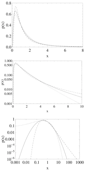
q→1= √2πσ and the usual log-Normal is recovered thereof (erfc stands for complementary error function). Typical plots for cases with q=4
5,q=1,q= 5
4are depicted in Fig. 1.
FIG. 1: Plots of Eq. (16)vs xforq= 45 (dotted line),q=1 (full line) andq=54(dashed line) in linear-linear scale (upper), log-linear (centre), log-log (lower).
The raw statistical moments, hxni ≡
Z ∞
0
xnp(x)dx, (18) can be analytically computed forq<1 giving [20],
hxni=
Γ[ν]exph−8γ2β
i
D−ν
γ √
2β
p
βνπσ(1−q)erfch−√1 2σ
1 1−q+µ
i, (19)
with β= 1
2σ2(1−q)2; γ=−
1+µ(1−q)
(1−q)2σ2 ; ν=1+
n 1−q,
(20) whereD−a[z] is the parabolic cylinder function [21]. For q>1, the raw moments are given by an expression quite sim-ilar to Eq. (19) with the argument of the erfc replaced by
1 √
2σ
1 1−q+µ
. However, the finiteness of the raw moments is not guaranteed for everyq>1 for two very related reasons. First, according to the definition ofD−ν[z],νmust be greater than 0. Second, the core of the probability density function, exp
−(lnqx−µ)
2
2σ2
, does not vanish in the limit ofxgoing to infinity∞,
lim x→∞exp
"
−(lnqx−µ) 2
2σ2
#
=exp
−γ 2
2
. (21)
This means that the limitp(x→∞) =0 is introduced by the normalisation factorx−q, which comes from redefining the Gaussian of variables,
y≡lnqx, (22)
as a distribution of variablesx. Because of that, if the moment surpasses the value ofq, then the integral (18) diverges.
4. EXAMPLES OF CASCADE GENERATORS
In this section, we discuss the upshot of two simple cases in which the dynamical process described in the previous sec-tion is applied. We are going to verify that the value ofq influences the nature of the attractor in probability space.
4.1. Compact distribution[0,b]
Let us consider a compact distribution for indentically and independently distributed variablesxwithin the interval 0 and b. Following what we have described in the preceding sec-tion, we can transform our generalised multiplicative process into a simple additive process ofyivariables which are now distributed in conformity with the distribution,
p′(y) =1
b[1+ (1−q)y]
q
1−q, (23)
withydefined between q−11 and b1−1−q−q1 ifq<1, whereasy ranges over the interval between−∞andb11−−q−q1whenq>1. Some curves for the special caseb=2 are plotted in Fig. 2.
If we look at the variance of this independent variable, σ2y=
y2− hµyi2, (24) which is the moment whose finitude plays the leading role in the Central Limit Theory, we verify that forq>3
2, we obtain a divergent value,
σ2y=
b2−2q
FIG. 2: Plots of the Eq. (23)vs y forb=2 and the values ofq
presented in the text.
Hence, ifq<3
2, we can apply the Lyapunov’s central Limit theorem and our attractor in the probability space is the Gaus-sian distribution. On the other hand, if q > 32, the L´evy-Gnedenko’s version of the central limit theorem [22] asserts that the attracting distribution is a L´evy distribution with a tail exponent,
α= 1
q−1. (26)
Furthermore, it is simple to verify that the interval 32,∞
ofq values maps onto the interval(0,2)ofαvalues, which is pre-cisely the interval of validity of the L´evy class of distributions that is defined by its Fourier Transform,
F
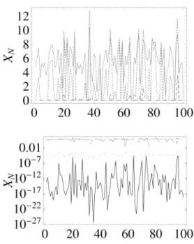
[Lα(Y)] (k) =exp−a|k|α. (27) In Fig. 3 we depict some sets generated by this process for different values ofq.4.2. q-log Normal distribution
In this example, we consider the case of generalised multi-plicative processes in which the variables follow aq-log Nor-mal distribution. In agreement with what we have referred to in Sec. 3, the outcome strongly depends on the value ofq. Consequently, in the associatedxspace, if we apply the gen-eralised process toN variablesy=lnqx(x∈[0,∞)) which follow a Gaussian-like functional1form with averageµand finite standard deviationσ,i.e.,∀q<1orq>3 in Eq.(16), the resulting distribution in the limit ofNgoing to infinity corre-sponds to the probability density function (16) withµ→N µ andσ2→Nσ2. In respect of the conditions ofqwe have just mentioned here above, theq-log normal can be seen as an asymptotic attractor, a stable attractor forq=1, and an un-stable distribution for the remaining cases with the resulting
1Strictly speaking, we cannot use the term Gaussian distribution because it
is not defined in the interval(−∞,∞). The limitations in the domain do affect the Fourier transform and thus the result of the convolution of the probability density function.
FIG. 3: Sets of random variables generated from the process (15) withN=100 andq=−1
2 (green), 0 (red), 1
2 (blue), 1 (black), 5 4
(magenta) in linear (upper panel) and log scales (lower panel). The generating variable is uniformly distributed within the interval[0,1] as is the same for all of the cases that we present. As visible, the value ofqdeeply affects the values ofXN=Z˜.
attracting distribution being computed by applying the con-volution operation.
5. FINAL REMARKS
In this manuscript we have introduced a modification in the multiplicative process that has enabled us to present a mod-ification on the log-Normal distribution as well as other dis-tributions with slow decay. This distribution is controlled by an extra-parameter,q, when it is compared with the regular 2-parameter log-Normal distribution, which can be dynamically related to a change in the multiplicative random process. Be-sides, it provides interesting mechanisms of on-off dynamics. Regarding further applications, it is known that the stan-dard log-normal distribution is unfitted for several data sets. This 3-parameter log-Normal probability function is expected to provide a better approach to these data [23].
[1] C. Tsallis, J. Stat. Phys.52, 479 (1988)
[2] C. Tsallis, Introduction to Nonextensive Statistical Mechanics: Approaching a Complex World (Springer, Berlin, 2009); Com-plexity, Metastability, and Nonextensivity: An International Conference edited by S. Abe, H. Herrmann, P. Quarati, A. Rapisarda, C. Tsallis, AIP Conf. Proc.965(2007); Complex-ity, Metastability and Nonextensivity, edited by C. Beck, G. Benedek, A. Rapisarda, C. Tsallis (World Scientific, Singa-pore, 2005);Nonextensive Entropy – Interdisciplinary Applica-tions, edited by M. Gell-Mann, C. Tsallis (Oxford University Press, New York, 2004)
[3] E.P. Borges, Physica A340, 95 (2004)
[4] L. Nivanen, A. Le Mehaute and Q.A. Wang, Rep. Math. Phys. 52, 437 (2003)
[5] E.P. Borges, Doctorate Thesis, CBPF, Rio de Janeiro (unpub-lished, 2004) [in Portuguese].
[6] S. Umarov, and C. Tsallis, Phys. Lett. A 372, 4874-4876 (2008); S. Umarov, S.M. Duarte Queir´os, e-print arXiv:0711.2550[cond-mat.stat-mech] (preprint, 2008) [7] S. Umarov, C. Tsallis, S. Steinberg, Milan J. Math, ;S. Umarov
and C. Tsallis,Complexity, Metastability, and Nonextensivity: An International Conference edited by S. Abe, H. Her-rmann, P. Quarati, A. Rapisarda, C. Tsallis, AIP Conf. Proc. 965, 34 (2007); S. Umarov, C. Tsallis, M. Gell-Mann and S. Steinberg, e-print arXiv:cond-mat/0606040 [cond-mat.stat-mech] (preprint, 2006) and e-print arXiv:cond-mat/0606038 [cond-mat.stat-mech] (preprint, 2006)
[8] M.S. Reis, J.C.C. Freitas, M.T.D. Orlando, E.K. Lenzi and I.S. Oliveira, Europhys. Lett.58, 42 (2002)
[9] C. Tsallis, Quimica Nova17, 468 (1994)
[10] S.M. Duarte Queir´os and C. Tsallis,Complexity, Metastability, and Nonextensivity: An International Conferenceedited by S. Abe, H. Herrmann, P. Quarati, A. Rapisarda, C. Tsallis, AIP Conf. Proc.965, 8 (2007);
[11] U. Frisch,Turbulence: The Legacy of A. Kolmogorov (Cam-bridge University Press, Cam(Cam-bridge, 1997); C. Beck, E.G.D Cohen, and H.L. Swinney, Phys. Rev. E72, 056133 (2005) [12] J. Feder, Fractals (Plenum, New York, 1988)
[13] B.B. Mandelbrot, Fractals and Scaling in Finance (Springer, New York, 1997)
[14] D. Stauffer, S.M. Moss de Oliveira, P.M.C. de Oliveira and J.M. de S´a Martins,Biology, Sociology, Geology by Computational Physicists,Vol. 1 (Elsevier, Amsterdam, 2006)
[15] Lognormal Distributions: Theory and Applications, edited by E.L. Crow and K. Shimizu (CRC Pess, New York, 1988) [16] R. Gibrat, Bull. Statist. G´en. Fr.19, 469 (1930)
[17] A.N. Kolmogorov, Dok. Acad. Nauk SSSR31, 99 (1941) [18] K.S. Fa, Chem. Phys.287, 1 (2003)
[19] A. Araujo, E. Guin´e,The Central Limit Theorem for Real and Banach Valued Random Variables(John Wiley & Sons, New York, 1980)
[20] I.S. Gradshteyn and I.M. Ryzhik, Table of Integrals, Series, and Products (Academic Press, New York, 1980),3.462.1
[21] http://functions.wolfram.com/HypergeometricFunctions/ ParabolicCylinderD/
[22] P. L´evy, Th´eorie de I’addition des variables al´eatoires
(Gauthierr-Villards, Paris, 1954)