www.geosci-model-dev.net/5/1009/2012/ doi:10.5194/gmd-5-1009-2012
© Author(s) 2012. CC Attribution 3.0 License.
Geoscientific
Model Development
Assessing climate model software quality: a defect density analysis
of three models
J. Pipitone and S. Easterbrook
Department of Computer Science, University of Toronto, Canada Correspondence to:J. Pipitone ([email protected])
Received: 1 January 2012 – Published in Geosci. Model Dev. Discuss.: 15 February 2012 Revised: 11 June 2012 – Accepted: 27 June 2012 – Published: 9 August 2012
Abstract.A climate model is an executable theory of the cli-mate; the model encapsulates climatological theories in soft-ware so that they can be simulated and their implications in-vestigated. Thus, in order to trust a climate model, one must trust that the software it is built from is built correctly. Our study explores the nature of software quality in the context of climate modelling. We performed an analysis of defect re-ports and defect fixes in several versions of leading global cli-mate models by collecting defect data from bug tracking sys-tems and version control repository comments. We found that the climate models all have very low defect densities com-pared to well-known, similarly sized open-source projects. We discuss the implications of our findings for the assess-ment of climate model software trustworthiness.
1 Introduction
In this paper we report on our investigation into the software quality of climate models. A study by Easterbrook and Johns (2009) of the software development practices at the UK Met Office Hadley Centre estimates an extremely low defect den-sity for the climate model produced there, which suggests an extraordinary level of software quality. Our purpose in this study is to conduct a rigorous defect density analysis across several climate models to confirm whether this high level of quality holds, and whether it is true of other models.
Defect density measures the number of problems fixed by the developers of the software, normalised by the size of the body of code. We chose defect density as our indi-cator of quality because it is well-known and widely used across the software industry as a rough measure of qual-ity, and because of its ease of comparison with published
statistics. Additionally, the measure is general and does not rely on many assumptions about how software quality should be measured, other than the notion that fewer defects indicate greater software quality.
2 Background
2.1 Measuring software quality
In software engineering research, software quality is not a simple, well-defined concept. Kitchenham and Pfleeger (1996) suggest that software quality can be viewed through five different lenses:
– Thetranscendental viewsees software quality as some-thing that can be recognised and worked towards, but never precisely defined nor perfectly achieved. This view holds that quality is inherently unmeasurable. – Theuser viewdescribes software quality by how well
the software suits the needs of its users. This view does not consider the construction of the software unless it has a bearing on the user experience.
– The manufacturing view considers quality as confor-mance to specifications and development processes. Measuring manufacturing quality is done through mea-suring defect counts and rework costs.
– The value-based view takes an economic perspective by equating software quality with what the customer is willing to pay for the software.
The product and manufacturing views are the dominant views adopted by software researchers (van Vliet, 2000). Software is seen as a product, produced by a manufactur-ing process, i.e. software development. This view enables the quality of a product to be measured independently of the manufacturingprocess. Quality is then either the extent to which the product or processconformsto predetermined quality requirements, or the extent to which the product or process improves over time with respect to those require-ments. Quality requirements are then made measurable by decomposing them into quality factors and subfactors. Each factor is then associated with specific metrics taken as in-dicating the degree to which that factor is present, and so indicating the degree of overall quality. Software quality is variously defined as “the degree to which a system, compo-nent or process meets specified requirements,” (IEEE, 1990), or more broadly as “the degree to which software possesses a desired combination of attributes” (IEEE, 1998).
These two perspectives on software quality have been for-malised in software engineering standards. ISO Std 9126 (ISO, 2001) and IEEE Std 1061 (IEEE, 1998) are both aimed at managing product conformance. The Capability Maturity Model (CMM/CMMI)1 is a framework for measuring and carrying out software development process improvement. ISO 9001 and related ISO 900x standards2 define how to manage and measure (software development) process confor-mance. Whilst these standards reflect the product and manu-facturing views in what aspects of software development they consider relevant to software quality, the standards do not prescribe specific quality measurements nor hold any spe-cific measures as necessarily better at indicating quality than others. Those choices and judgements are left as tasks for individual projects.
2.2 Scientific software development
There is a long history of software research focused on in-dustrial and commercial software development but it is only recently thatscientific software development has been seen as an important area of research (Kelly, 2007). There is ev-idence to show that scientific software development has sig-nificant differences from other types of software develop-ment.
Segal and Morris (2008) and Segal (2008) point to two ma-jor differences. Experimentation and trial-and-error work is an essential part of the development process because the soft-ware is built to explore the unknown. It is often impossible to provide complete requirements for the software upfront, and
1See http://www.sei.cmu.edu/cmmi/
2See http://www.iso.org/iso/iso_catalogue/management_
standards/quality_management.htm
in fact, the requirements are expected to emerge and change over the lifetime of the project as the understanding of the science evolves. Partly because of this, the scientists must develop the software themselves, or be intimately involved, since it would be impossible to build the software correctly without their guidance and knowledge.
In a study of high-performance computing (HPC) commu-nities, Basili et al. (2008) find that scientists value scientific output as the highest priority and make decisions on program attributes accordingly. For instance, an increase in machine performance is often seen as the opportunity to add scientific complexity to their programs, not as an opportunity to save on execution time (since that may not serve as great a scien-tific purpose). They report that scientists recognised software quality as both very important and extremely challenging. They note that the techniques used are “qualitatively differ-ent for HPC than for traditional software developmdiffer-ent”, and that many software engineering techniques and tools, such as interactive debuggers, are simply not usable in their environ-ment.
In summary, scientific software development (under which climate modelling falls) is markedly different from the tradi-tional domains studied by software researchers. It works with few upfront requirements and a design that never truly settles since it must adapt to constant experimentation.
This raises the question: what does software quality mean in the climate modelling context?
2.3 The problem of software quality in scientific software
Stevenson (1999) discusses a divide between the software research community and the scientific community as it ap-plies to scientists building large-scale computer simulations as their primary research apparatus. Stevenson raises the con-cern that because the primary job of a scientist is to do sci-ence, software engineering notions of quality do not apply to software constructed as part of a scientific effort. This is because of fundamentally incompatible paradigms: scien-tists are concerned with the production of scientific insight, while software engineers are concerned with the manufac-turing process that produces software. Stevenson argues that for the termsoftware qualityto have meaning in the scien-tific domain, our notions of quality must be informed by our understanding of the requirement for insightand all that it entails.
executable implementation of the theoretical model; in our case, climate model code)3. Computational scientists study the behaviour of the calculational system to gain insight into the workings of the theoretical system, and ultimately the ob-servational system.
Two basic kinds of activity ensure that the systems cor-respond to one another.Validationis the process of check-ing that the theoretical system properlyexplainsthe observa-tional system, andverificationis the process of checking that the calculational system correctly implements the theoretical system. The distinction between validation and verification is expressed in the questions, “Are we building the right thing?” (validation) and, “Are we building the thing right?” (verifica-tion). Stevenson also uses the termcomplete validation to refer to checking all three systems – that is, to mean that "we compute the right numbers for the right reasons."
Stevenson describes two types of quality with respect to the above model of computational science.Intrinsic quality is "the sum total of our faith in the system of models and ma-chines." It is an epistemological notion of a good modelling endeavour; it is what we are asking about when we ask what needs to be present in any theoretical system and any im-plementation for us to gain insight and knowledge.Internal qualityapplies to a particular theoretical and calculational system, and asks how good our model and implementation is in its own right. For a mathematician, internal quality may relate to the simplicity or elegance of the model. For a com-puter scientist or engineer, internal quality may relate to the simplicity or extensibility of the code.
We have seen that, from one perspective, scientific insight is the ultimate measure of the overall quality of a scientific modelling endeavour. Meaningful insight depends upon the-oretical and calculational systems corresponding in sensible ways to each other, and ultimately to the observational sys-tem under study. So, the “correctness” of our models is bound up with our notion of quality: what are the “right numbers”? How do we know when we see them? The conceptual ma-chinery for approaching these questions is discussed suc-cinctly by Hook (2009) and Hook and Kelly (2009).
Hook divides error, the “difference between measured or calculated value of a quantity and actual value”, into acknowledged error andunacknowledged error. Acknowl-edged errors “are unavoidable or intentionally introduced to make a problem tractable” whereas unacknowledged errors “result from blunders or mistakes”. Defining a theoretical model and refining it into a calculational model necessar-ily introduces acknowledged error. This error may come in the form of uncertainties in experimental observations, ap-proximations and assumptions made to create a theory of
3There are alternatives to these terms which Stevenson does not
mention. The termmodelis used both to refer to the theoretical
sys-tem at times, and at other times to refer to the calculational syssys-tem.
The termsimulationis only used to refer to thecalculational
sys-tem.
the observational system, truncation and round-off errors that come from algorithmic approximations and discretizations of continuous expressions, the implementation – i.e. program-ming – of those algorithms, or even from compiler optimiza-tions made during translation to machine code. Unacknowl-edged errors may appear at any step along the way because of mistakes in reasoning or misuse of equipment.
There are two fundamental problems that make impossi-ble the traditional notion of testing by way of directly com-paring a program’s output to an expected value. The first is what Hook terms thetolerance problem: it is impossible, or very difficult, to tell if errors in output are completely free of unacknowledged error since it may be difficult to bound ac-knowledged error, and even with a bound on acac-knowledged error it is impossible to detect unacknowledged errors that fall within those bounds. In short, because there is a range of acknowledged error in the output, some unacknowledged error cannot reliably be detected.
The second problem is theoracle problem: “available ora-cles are problematically imprecise and limited”. That is, for certain inputs there may not exist a source of precise ex-pected outputs with which to compare a program’s output. For a computational scientist, many of the important out-puts of scientific software are theresultsof an experiment. If the output was always known beforehand, then the scientists would not be engaging in science. As a result of the oracle problem, scientists may have to rely on educated guesses, in-tuition, and comparison to available data in order to judge the “correctness” of their software.
In summary, for any given input there may be no accurate expected output values (the oracle problem); and because of inherent error in the output, unacknowledged errors may be undetectable (the tolerance problem). These problems do not suggest that building correct models is impossible, but that in the scientific software domain we must redefine correctness so as to take into account these problems. That is, we cannot accept that an evaluation of a model’s correctness consists only of comparing output to expected values.
How, then, should climate model quality be judged? This is the problem of quality in scientific software which the present work explores, albeit only partially since we concern ourselves with the question ofsoftwarequality and not theo-retical quality.
that prevent the study of scientific software quality from be-ing a straightforward matter of applybe-ing existbe-ing software en-gineering knowledge to a new domain. Instead, they suggest that software researchers work with scientists to learn more about their development context, and establish which soft-ware development techniques can be used directly and what has to be adapted or created. With respect to software cor-rectness, they ask:
“At this point, we don’t have a full list of factors that contribute to correctness of scientific software, particularly factors in areas that a software engineer could address. What activities can contribute to factors of importance to correctness? How effective are these activities?" (Kelly and Sanders, 2008)
We will revisit these questions in Sect. 5.2.
Assessing the quality of scientific software may be tricky, but is it needed? Hatton (1997b) performed a study analysing scientific software from many different application areas in order to shed light on the answer to this question. Hatton’s study involved two types of quality tests. The first test, T1, involved static analysis of over 100 pieces of scientific soft-ware. This type of analysis results in a listing of “weak-nesses”, or static code faults – i.e., known “misuse[s] of the language which will very likely cause the program to fail in some context". The second test, T2, involved comparing the output of nine different seismic data processing programs, each one supposedly designed to do the same thing, on the same input data. Hatton found that the scientific software analysed had plenty of statically detectable faults, that the number of faults varied widely across the different programs analysed, and that there was significant and unexpected un-certainty in the output of this software: agreement amongst the seismic processing packages was only to one signifi-cant digit. Hatton concludes that, "taken with other evidence, the T experiments suggest that the results of scientific cal-culations carried out by many software packages should be treated with the same measure of disbelief researchers have traditionally attached to the results of unconfirmed physical experiments." Thus, if Hatton’s findings are any indication of quality of scientific software in general, then improvements in software quality assessment of scientific software is dearly needed.
2.4 Climate model development
Theclimateis “all of the statistics describing the atmosphere and ocean determined over an agreed time interval.”Weather, on the other hand, is the description of the atmosphere at a single point in time. Climate modellers are climate scientists who investigate the workings of the climate by way of com-puter simulations:
“Any climate model is an attempt to represent the many processes that produce climate. The objective is to under-stand these processes and to predict the effects of changes and interactions. This characterization is accomplished by
describing the climate system in terms of basic physical, chemical and biological principles. Hence, a numerical model can be considered as being comprised of a series of equations expressing these laws." (McGuffie and Henderson-Sellers, 2005)
Climate modelling has also become a way of answering questions about the nature of climate change and about pre-dicting the future climate and, to a lesser extent, the predic-tion of societal and economic impacts of climate change.
Climate models come in varying flavours based on the level of complexity with which they capture various physical processes or physical extents. GCMs (“global climate mod-els” or “general circulation modmod-els”) are the most sophis-ticated of climate models. They are numerical simulations that attempt to capture as many climate processes as possible with as much detailed output as possible. Model output con-sists of data for points on a global 3D grid as well as other diagnostic data for each time-step of the simulation. Whilst GCMs aspire to be the most physically accurate of models, this does not mean they are always the most used or useful; simpler models are used for specific problems or to “provide insight that might otherwise be hidden by the complexity of the larger models” (McGuffie and Henderson-Sellers, 2005; Shackley et al., 1998). In this paper we focus on the develop-ment of GCMs for two reasons: they are the most complex from a software point of view; and, to the extent that they pro-vide the detailed projections of future climate change used to inform policy making, they are perhaps the models for which software quality matters the most.
GCMs are typically constructed by coupling together sev-eral components, each of which is responsible for simulating the various subsystems of the climate: atmosphere, ocean, ice, land, and biological systems. Each component can often be run independently to study the subsystem in isolation. A special model component, the coupler, manages the transfer of physical quantities (energy, momentum, air, etc.) between components during the simulation. As GCMs originally in-cluded only atmosphere and ocean components, models that include additional Earth system processes are often referred to as Earth system models (ESMs). For simplicity, hereafter, we will use the phraseclimate modelto mean both GCMs and ESMs.
In order to facilitate experimentation, climate models are highly configurable. Entire climate subsystem components can be included or excluded, starting conditions and physical parameterizations specified, individual diagnostics turned on or off, as well as specific features or alternative implementa-tions of those features selected.
what we have already summarised above about general scien-tific software development in a high-performance computing environment.
Easterbrook and Johns find that evolution of the software and structure of the development team resemble those found in an open source community even though the centre’s code is not open nor is development geographically distributed. Specifically, the domain experts and primary users of the software (the scientists) are also the developers. As well, there are a small number of code owners who act as gate-keepers over their component of the model. They are sur-rounded by a large community of developers who contribute code changes that must pass through an established code re-view process in order to be included in the model.
Easterbrook and Johns also describe the verification and validation (V&V) practices used by climate modellers. They note that these practices are “dominated by the understanding that the models are imperfect representations of very com-plex physical phenomena.” Specific practices include the use ofvalidation notes: standardized visualisations of model out-puts for visually assessing the scientific integrity of the run or as a way to compare it with previous model runs. An-other V&V technique is the use of bit-level comparisons be-tween the output of two different versions of the model con-figured in the same way. These provide a good indicator of reproducibility on longer runs, and strong support that the changes to the calculational model have not changed the the-oretical model. Finally, results from several different models are compared. Organized model intercomparisons are con-ducted with models from several organisations run on simi-lar scenarios4. Additionally, the results from several different runs of the same model with perturbed physical parameters are compared in modelensemble runs. This is done so as to compare the model’s response to different parameteriza-tions, implementaparameteriza-tions, or to quantify output probabilities. Easterbrook and Johns conclude that “overall code quality is hard to assess”. They describe two sources of problems: configuration issues (e.g. conflicting configuration options), and modelling approximations which lead to acknowledged error. Neither of these are problems with the code per se.
3 Approach
In this study we analysed defect density for three differ-ent models: two fully coupled general circulation mod-els (GCMs) and an ocean model. For comparison, we also an-alyzed three unrelated open-source projects. We repeated our analysis for multiple versions of each piece of software, and we calculated defect density using several different methods. There are a variety of methods for deciding on what consti-tutes a defect and how to measure the size of a software prod-uct. This section makes explicit our definition of a defect and
4See http://cmip-pcmdi.llnl.gov/ for more information.
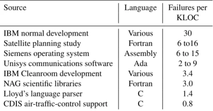
Table 1.Post-delivery problem rates as reported by Pfleeger and Hatton (1997)
Source Language Failures per
KLOC
IBM normal development Various 30
Satellite planning study Fortran 6 to16
Siemens operating system Assembly 6 to 15
Unisys communications software Ada 2 to 9
IBM Cleanroom development Various 3.4
NAG scientific libraries Fortran 3.0
Lloyd’s language parser C 1.4
CDIS air-traffic-control support C 0.8
product size, and explains in detail how we conducted our study.
We also compare our results with defect density rates re-ported in the literature, typically calculated as the number of failures encountered (or defects discovered) after deliv-ery of software to the customer, per thousand lines of source code (KLOC). For example, Pfleeger and Hatton (1997) list a number of published post-delivery defect rates, which we reproduce in Table 1. Hatton (1997a) states: “three to six de-fects per KLOC represent high-quality software.” Li et al. (1998) state that “leading edge software development or-ganizations typically achieve a defect density of about 2.0 defects/KLOC”. The COQUALMO quality model (Chulani and Boehm, 1999), which bases its interpretation of defect density on the advice of industry experts, suggests that high software quality is achieved at a post-release defect density of 7.5 defects/KLOC or lower.
3.1 Selection process
Convenience sampling and snowballing were used to find cli-mate modelling centres willing to participate (Fink, 2008). We began with our contacts from a previous study (East-erbrook and Johns, 2009), and were referred to other con-tacts at other centres. In addition, we were able to access the code and version control repositories for some centres anony-mously from publicly available internet sites.
We only considered modelling centres with large enough modelling efforts to warrant a submission to the IPCC Fourth Assessment Report (Solomon et al., 2007). We used this cri-teria because the modelling centres were well-known, and we had access to the code, project management systems, and developers. In the interests of privacy, the modelling centres remain anonymous in this report. We use the identifiers C1, C2, and C3 to refer to the three models we studied.
– theApacheHTTPD5webserver, which has been widely studied as an example of high quality open source soft-ware;
– theVisualization Toolkit (VTK)6, a widely used open source package for scientific visualization;
– theEclipseproject, an open source Integrated Develop-ment EnvironDevelop-ment, for which Zimmermann et al. (2007) provide a detailed defect density analysis.
3.2 Terminology
For the remainder of this paper, we adopt the following ter-minology:
– Erroris the difference between a measured or computed quantity and the value of the quantity considered to be correct.
– Acode faultis a mistake made when programming; it is "a misuse of the language which will very likely cause the program to fail in some context" (Hatton, 1997b). – Afailureoccurs when a code fault is executed (Hook,
2009).
– The termsdefectandbugare commonly used to refer to failures or faults, or both. We use these terms to mean both failures and faults, unless specified otherwise. – Defect reportsare reports about faults or failures,
typi-cally recorded in a bug tracking system, along with doc-umentation on the resolution of the problem.
– Adefect fixis any change made to the code to repair a defect, whether or not a defect report was documented. 3.2.1 Identifying defects
One approach to measuring software defects is to count each documented report of a problem filed against a software product. This approach has the drawback of ignoring those defects that are not formally reported, but which are found and fixed nonetheless. Since we did not have information on the bug reporting practices for every model we studied, we broadened our characterization of a defect fromreported and fixed problemstoany problem fixed. Hence, in addition to examining defect reports, we examined the changes made to the code over a given period to identify those that were intended to repair a defect. This broader analysis reflects an operational definition of a software defect as “any problem that is worth fixing”.
Defect reports are usually easy to identify, since they are labeled and stored in a project database which can be queried directly. We consider only those reports specifically labeled
5http://httpd.apache.org/
6http://www.vtk.org/
1. CT : BUGFIX083 : add the initialisation
of the prd 2D array in the xxxxx subroutine
2. xxxx_bugfix_041 : SM : Remove unused
variables tauxg and tauyg
3. Correct a bug in ice rheology, see ticket
#78
4. Correct a bug and clean comments in
xxxxx, see ticket #79
5. Ouput xxxx additional diagnostics at the
right frequency, see ticket:404
6. Initialization of passive tracer trends
module at the right place, see ticket:314
7. additional bug fix associated with
changeset:1485, see ticket:468
8. CT : BUGFIX122 : improve restart case
when changing the time steps between 2 simulations
9. Fix a stupid bug for time splitting and
ensure restartability for dynspg_ts in addition, see tickets #280 and #292
10. dev_004_VVL:sync: synchro with trunk
(r1415), see ticket #423
Fig. 1.A sample of version control log messages indicating a defect fix. Redacted to preserve anonymity.
as defects (as opposed to enhancements or work items) as well as being labeled as fixed (as opposed to unresolved or invalid).
Identifying defects fixes is more problematic. Although all code changes are recorded in a version control repository, the only form of labeling is the use of free-form revision log messages associated with each change. We used an informal technique for identifying defect fixes by searching the revi-sion log messages for specific keywords or textual patterns (Zimmermann et al., 2007). We began by manually inspect-ing a sample of the log messages and code changes from each project. We identified which revisions appeared to be defect fixes based on our understanding of the log message and details of the code change. We then proposed patterns (as regular expressions) for automatically identifying those log messages. We refined these patterns by sampling the match-ing log messages and modifymatch-ing the patterns to improve re-call and precision. The pattern we settled on matches mes-sages that contain the strings “bug”, “fix”, “correction”, or “ticket”; or contain the “#” symbol followed by digits (this typically indicates a reference to a report ticket). Figure 1 shows a sample of log messages that match this pattern.
1998 1999 2000 2001 2002 2003 2004 2005 2006 2007 2008 2009 2010 Time (year)
VTK Apache C3 C2 C1
Pro
jec
t
5- 0-1 5-
0-2 5-
0-3 5-
0-4 5-
2-0 5-
2-1 5-
4-0 5-
4-1 5-
4-2 1.3.
6
2.0. 35
2.1. 7
2.2. 10
2.3. 4
v25 v71v86 v141
v0 v1 v2 v3 v4 v5 v6 v7 v8 v33 v36 v40 v38 v39
Repository timeline
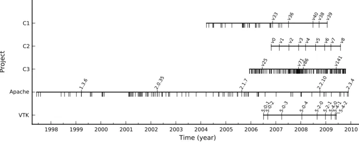
Fig. 2.Project repository time lines. Candidate versions are marked on the timelines with downward ticks, and analysed versions are labelled.
we only had access to the version control repository we used the tool CVSANALY7to build an SQLITE8database of the repository items. This database includes tables for: the log messages, tags, and all of the files and folders. One centre provided us with a snapshot of theirt r ac9 installation and
repository. We used the database powering thet r ac
installa-tion (also based on SQLITE) as it stores the repository data in a similar way to CVSANALY.
3.2.2 Measuring product size
In order to normalize defect counts, it is necessary to select a method for calculating product size. The size of a software product is typically measured in terms of code volume (e.g., source lines of code) or function points (a measure of the functionality provided by the source code). Source lines of code (SLOC) can be measured automatically. In contrast, function points, which are considered to be a more accu-rate measurement of the essential properties of a piece of software (Jones, 2008), rely on subjective judgment, and are time-consuming to assess for large software systems. There-fore, we chose to use the source lines of code metric for its ease of measurement and repeatability (Jones, 2008; Park, 1992).
There are two major types of source lines of code mea-sures: physical, and logical. The Physical SLOC measure views each line of text in a source file as a potential line of code to be counted. The physical SLOC measure we re-port counts all lines except blank lines and lines with only comments. TheLogical SLOCmeasure ignores the textual formatting of the source code and considers each statement
7http://tools.libresoft.es/cvsanaly
8http://sqlite.org/
9http://trac.edgewall.org/
to be a line of code. In this study we report both of these mea-sures but we use the physical SLOC measure in our calcula-tion of defect density since we feel it as a more reproducible and language-neutral measure.
We used the CODECOUNT10tool to count source lines of code for all of our projects. We determined which source files to include in the count based on their extension:.F, .f, .f90for Fortran files and .c, .cpp,.h, and .hppfor C/C++ projects). We included other files if we knew from conversations with the developers that they contained code (for example, model C2 contained Fortran code in certain.h files). Additionally, we analysed the source files without per-forming any C preprocessing and so our line counts include C preprocessing directives and sections of code that might not appear in any specific model configuration.
3.2.3 Calculating defect density
Defect density is loosely defined as the number of defects found in a product divided by the size of the product. De-fects are discovered continuously throughout the develop-ment and use of a software product. However, product size changes discretely as modifications are made to the source code. Thus, in order to calculate the defect density of a prod-uct we must be able to associate defects to a particular ver-sion of the product. We use the termversionto refer to any snapshot of model source code whose size we can measure and assign defects to. A version in this sense does not nec-essarily refer to a public release of the product since defects can be both reported and fixed on unreleased or internally released versions.
In general, we attempted to limit the versions we anal-ysed to major product releases only. We began with a pool of
candidate versions populated from the source code revisions in the version control repository. Where possible, we used only those versions indicated as significant by the developers through personal communication. Otherwise, we narrowed the pool of candidate versions to only those revisions that were tagged in the repository (models C1, C3, and compara-tors HTTPDand VTK) under the assumption that tags indi-cated significance. We further narrowed our candidate ver-sions by selecting only those tagged reviver-sions that had asso-ciated defect reports. We assumed that reports are typically logged against major versions of the product. We attempted to match repository tag names to the version numbers listed in the issue report database for the project. Where there was ambiguity over which tag version to choose we chose the old-est one11. We will refer to the remaining candidate versions – those that were included in our analysis – asselected ver-sions. Figure 2 shows a time line for each project marking the selected versions, as well as the other candidate versions we considered. To maintain the anonymity of the models, we have used artificial version names rather than the repository tags or actual model version numbers.
Assigning a defect to a product version can be done in several ways. In a simple project, development proceeds se-quentially, one release at a time. Simplifying, we can make the assumption that the defects found and fixed leading up to or following the release date of a version are likely de-fects in that version. Dede-fects which occur before the release date are calledpre-release defectsand those which occur af-terwards are calledpost-release defects. One method for as-signing defects to a product version is to assign all of the pre-and post-release defects that occur within a certain time in-terval of a version’s release date to that version. We call this methodinterval assignment. We used an interval duration of six months to match that used by Zimmermann et al. (2007). An alternative method is to assign to a version all of the defects that occur in the time span between its release date and the release date of the following version. We call this methodspan assignment.
A third and more sophisticated method is used in Zimmer-mann et al. (2007), whereby defect identifiers are extracted from the log messages of fixes, and the version label from the ticket is used to indicate which version to assign the defect to. We call this methodreport assignment.
We used all three assignment methods to calculate defect density.
11For instance, in one project there were repository tags of the
form <release_number>_beta_<id>, and a report version name of the form <release_number>_beta. Our assumption is that devel-opment on a major version progresses with minor versions being tagged in the repository up until the final release.
0 500 1000 1500 2000
Lines of code (KLOC) 3.0
2.1 2.0 VTK-5-4-2 VTK-5-4-1 VTK-5-4-0 VTK-5-2-1 VTK-5-2-0 VTK-5-0-4 VTK-5-0-3 VTK-5-0-2 VTK-5-0-1 2.3.4 2.2.10 2.1.7 2.0.35 v141 v86 v71 v25 v8 v7 v6 v5 v4 v3 v2 v1 v0 v39 v38 v40 v36 v33
Version
Eclipse VTK Apache C3 C2 C1
logical physical total
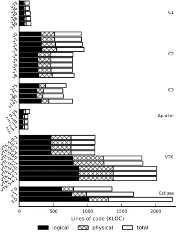
Fig. 3.Lines of code measurements for each project.
4 Results
Figure 3 displays the physical, logical and total line count for each project, and Table 2 lists the median defect densities of each project version using the physical product size measure-ment. For Eclipse, we extracted defect counts for each ver-sion by totalling the defects found across all of the plug-ins that compose the Eclipse JDT product using the data pub-lished by Zimmermann et al. (2007).
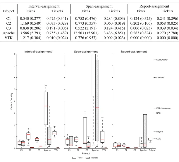
Figure 4 displays the post-release defect densities of the projects we analysed, with several of the listed projects from Table 1 marked down the right hand side of the chart for com-parison. Both the fix- and report-defect densities are included for each assignment method.
Regardless of whether we count fixes or reported defects, and regardless of the assignment method used, the median defect density of each of the climate models is lower, often significantly, than the projects listed in Table 1. Similarly, the median model defect density is lower, often significantly, than the comparator projects.
Table 2. Median project defect density (interquartile range in parenthesis) of analysed versions under different defect assignment methods.
Interval-assignment Span-assignment Report-assignment
Project Fixes Tickets Fixes Tickets Fixes Tickets
C1 0.540 (0.277) 0.475 (0.341) 0.752 (0.476) 0.284 (0.803) 0.124 (0.325) 0.241 (0.296)
C2 1.169 (0.549) 0.073 (0.029) 0.773 (0.357) 0.060 (0.019) 0.202 (0.106) 0.058 (0.025)
C3 0.838 (0.206) 0.191 (0.006) 0.522 (2.191) 0.124 (0.415) 0.006 (0.023) 0.039 (0.034)
Apache 3.586 (2.793) 0.755 (1.489) 12.503 (15.901) 3.436 (6.851) 0.283 (0.824) 0.270 (2.780)
VTK 1.217 (0.304) 0.010 (0.024) 0.776 (0.957) 0.009 (0.023) 0.000 (0.000) 0.000 (0.000)
C1 C2 C3 Apache VTK 0
1 2 3 4 5 6 7 8
Defect Density
Interval-assignment
C1 C2 C3 Apache VTK Project
Span-assignment
C1 C2 C3 Apache Eclipse NAG
CDIS Lloyd's IBM cleanroom Siemens COQUALMO
Report-assignment
Fixes Tickets
Fig. 4.Defect density of projects by defect assignment method. Previously published defect densities from Table 1 are shown on the right.
defects may be reported whereas minor defects are simply found and fixed.
5 Discussion
Each of the comparator projects we chose is a long-lived, well-known, open-source software package. We have good reason to believe that they are each of high quality and rig-orously field-tested. Thus, our results suggest that the soft-ware quality of the climate models investigated is as good as, or better than, the comparator open source projects and de-fect density statistics reported in the literature. In addition, to the best of our knowledge, the climate modelling centres that produced the models we studied are representative of major modelling centres. This suggests that climate models from other centres may have similarly low defect densities.
Our results are surprising in light of previous studies of scientific software development, which show how volatile and vague their requirements are (Kelly, 2007; Segal and
Morris, 2008; Segal, 2008; Carver et al., 2007). Our results suggest that the climate modellers have produced very high quality software under uncertain conditions with little in the way of guidance from the software engineering community.
Notwithstanding issues of construct validity that we dis-cuss in Sect. 5.1.4, there are a number of possible explana-tions for low defect densities in the models. We offer the fol-lowing hypotheses:
2. Rigorous development process.As we have discussed, scientific correctness is paramount for climate mod-ellers. This concern is reflected in an extremely rigorous change management process where each code change undergoes intense scrutiny by other modellers (Easter-brook and Johns, 2009). Under this hypothesis, the rel-ative effort put into inspecting code changes leads to fewer introduced defects.
3. Domination by caution.Fear of introducing defects may cause modellers to proceed with such caution as to slow down model development significantly, providing more time to consider the correctness of each code change. This hypothesis suggests we would also expect to see a lower code churn per developer per unit time than in commercial software practices12. If true, it might also mean that modellers are sacrificing some scientific pro-ductivity in return for higher quality code.
4. Narrow usage profile.Our comparators are general pur-pose tools (i.e. a numerical library, an IDE, and a web-server) whereas, this hypothesis holds, even though cli-mate models are built to be extremely flexible, they are most often used and developed for a much smaller set of scenarios than they are capable of performing in. That is, only a limited number of the possible model con-figurations are regularly used in experiments. Develop-ment effort is concentrated on the code paths supporting these configurations, resulting in designed, well-tested and consequently, high quality code. However, this hypothesis would suggest the models may be rel-atively brittle, in that the less frequently used configura-tions of the models may include many more unnoticed code faults (unacknowledged errors). If code routines that are rarely used make up a significant proportion of the code size, then the defect density count will be skewed downwards.
5. Intrinsic sensitivity/tolerance. This hypothesis posits that there are intrinsic properties of climate models that lead to the production of high quality software inde-pendent of the skill of the development team. For in-stance, climate models may be sensitive to certain types of defects (those that change climate dynamics or nu-merical stability, for example). These defects appear as obvious failures (e.g. a crash, or numerical blowup) or improbable climate behaviours, and are therefore fixed at the time of development, resulting in fewer defect re-ports and fixes. At the same time, we have evidence that climate model behaviour is robust. One climate mod-eller we interviewed explained that the climate is a “het-erogeneous system with many ways of moving energy
12although this may be masked by certain coding practices,
(e.g. cut-and-paste, lack of granularity) where conceptually small changes result in disproportionate source code changes.
around from system to system” which makes the theo-retical system being modelled “tolerant to the inclusion of bugs.” The combination of both factors means that code defects are either made obvious (and so immedi-ately fixed) or made irrelevant by the nature of climate models themselves and therefore never reported as de-fects.
6. Successful disregard.Compared to other domains, cli-mate modellers may be less likely to consider certain defects important enough to report or even be seenas defects. The culture of emphasizing scientific correct-ness may lead modellers to ignore defects which do not cause errors in correctness (e.g. problems with usability, readability or modifiability of the code), and defects for which there are ready workarounds (e.g output format errors). In other words, modellers have "learned to live with a lower standard" of code and development pro-cesses simply because they are good enough to produce valid scientific results. A net result may be that climate modellers incur higher levels oftechnical debt(Brown et al., 2010) – problems in the code that do not affect correctness, but which make the code harder to work with over time.
Several of these hypotheses call into question the use of standard measures of defect density to compare software quality across domains, which we will consider in depth in the following section.
5.1 Threats to validity
5.1.1 Overall study design
We do not yet understand enough about the kinds of climate modelling organisations to make any principled sampling of climate models that would have any power to generalize to all climate models. Nevertheless, since we used convenience and snowball sampling to find modelling centres to partici-pate in our study, we are particularly open to several biases (Fink, 2008):
– Modelling centres willing to participate in a study on software quality may be more concerned with software quality themselves.
– Modelling centres which openly publish their climate model code and project artifacts may be also be more concerned with software quality.
One of the models used in the study (C1) is an ocean model rather than a full climate model. Even though this particular model component is developed as an independent project, it is not clear to what extent it is comparable to a full GCM.
were large enough and well-known enough to provide an in-tuitive comparison to the climate models.
Our choice to use defect density as a quality indicator was made largely because of its place as ade factorough measure of quality, and because of existing publications to compare to. Gauging software quality is known to be tricky and sub-jective and most sources suggest that it can only accurately be done by considering a wide range of quality indicators (Jones, 2008; IEEE, 1998; ISO, 2001; Hatton, 1995). Thus, at best, our study can only hope to present a very limited view of software quality.
5.1.2 Internal validity
The internal validity of the defect assignment methods (i.e. interval- and span-assignment) is threatened by the fact that we chose to view software development as proceeding in a linear fashion, from one major version to the next. This view assumes a defect found immediately before and after a re-lease date is a defect in that rere-lease. However, when several parallel branches of a project are developed simultaneously, as some projects in our study were, this flattened view of de-velopment is not able to distinguish amongst the branches. We may have incorrectly assigned a defect to a version in a different branch if the defect’s date was closer to the ver-sion’s release date than to the version the defect rightfully is associated with.
In addition, we assumed a 1:1 mapping between defect in-dicators and defects. We did not account for reports or ver-sion control check-ins that each refer to multiple defects, nor for multiple reports or check-ins that, together, indicate only one defect.
Finally, we did not perform any rigorous analysis of recall and precision of our fix identification method. This means we cannot say whether our counts are over- or under-estimates of the true number of check-ins that contain defect fixes.
5.1.3 External validity
The external validity of our assignment methods depends on correctly picking repository versions that correspond to ac-tual releases. If a version is used that is not a release, then it is not clear what is meant by pre-release and post-release defects, and whether they can be compared. For several of the projects we made educated guesses as to the versions to select (as described in Sect. 3), and so we may have classified some defects as post-release defect that may more rightly be classified as pre-release defects had we chosen the correct version. Similarly, if there were no releases of the project made in our repository snapshot, we used intermediate ver-sions. This makes it difficult to justify comparing defect rates since pre- and post-release are not clearly defined.
Our definition of a defect as “anything worth fixing” was a convenient definition for our purposes but it has not been val-idated in the field, and it is even unclear that it corresponds to
our own intuitions. What about defects that are found but not worth fixing right then and there? We confront this question in Sect. 5.2.
Finally, there are many small differences between the way we carried out our identification of code fixes and that of Zimmermann et al. (2007). In their study, they did not rig-orously specify the means by which check-in comments were identified as fixes; they only gave a few examples of common phrases they looked for. We were forced to invent our own approximation. Furthermore, for report-assignment, Zimmermann et al. (2007) used the first product version listed in a report’s history as the release date to associate de-fects with. Since we did not have access to the report history for every project we analysed, we only considered the prod-uct version as of the date we extracted the report informa-tion. As well, Zimmermann et al. (2007) only counted defects that occurred within 6 months of the release date whereas we counted all defects associated with a report version. Thus, it is not clear to what extent we can rightly compare our results. 5.1.4 Construct validity
As we have mentioned, defect density is thede facto infor-mal measure of software quality but it is by no means consid-ered a complete or entirely accurate measure. Hatton (1997a) says:
“We can measure the quality of a software system by its de-fect density – the number of dede-fects found per KLOC over a period of time representing reasonable system use. Although this method has numerous deficiencies, it provides a reason-able though rough guide."
The question we explore in this section is: to what ex-tent can we consider defect density even a rough indicator of quality?
We suggest the following aspects which make the defect density measure open to inconsistent interpretation:
– Finding, fixing, and reporting behaviour.In order to be counted, defects must be discovered and reported. This means that the defect density measure depends on the testing effort of the development team, as well as the number of users, and the culture of reporting defects. An untested, unused, or abandoned project may have a low defect density but an equally low level of quality. – Accuracy and completeness of repository comments
or defect reports are accurate.There is good reason to believe that these data sources contain many omissions and inaccuracies (Aranda and Venolia, 2009).
– Product use.The period of time over which to collect defects (e.g. “reasonable system use”) is unclear and possibly varies from release to release.
project even make major releases or does it have contin-uous incremental releases?
– Product size.There are many ways of evaluating the product size, which one should we use and is it replica-ble? Can it account for the expressiveness of different languages, formatting styles, etc?
– Criticality and severity. Are all defects counted equally, or certain severity levels ignored?
When we use the defect density measure to compare soft-ware quality between projects, we are implicitly making the assumption that these factors are similar in each project. If they are not – and without any other information we have no way of knowing – then we suggest the defect density mea-sure is effectively meaningless as a method of comparing the software quality, even roughly, between products. There is too much variability in the project conditions for a single in-terval measure to account for or express.
Even if all our concerns above are taken into account, we cannot rightly conclude that a product with low defect den-sity is, even roughly, of better quality than one with a higher defect density. Jones (2008) states that whilst software defect levels and user satisfaction are correlated, this relationship disappears when defect levels are low: having fewer defects does not tell us anything about the presence of favourable quality attributes.
Our focus on defect density emphasizes code correctness over and above other aspects of software quality. Of particu-lar concern to the climate modelling community is the extent to which poorly written or poorly structured code may slow down subsequent model development and hence may reduce scientific productivity, even it if works perfectly. Our study did not attempt to measure these aspects of software quality. In Sect. 5.2 we will discuss ideas for future studies to help discover quality factors relevant in the climate modelling do-main.
5.2 Future work
Many of the limitations to the present study could be over-come with more detailed and controlled replications. Mostly significantly, a larger sample size both of climate models and comparator projects would lend to the credibility of our de-fect density and fault analysis results.
As we have mentioned elsewhere, assessing software qual-ity is not a simple matter of measuring one or two qualqual-ity indicators, but neither is it clear howanycollection of mea-surements we could make could give us an assessment of software quality with confidence. Hatton (1995) remarks:
“There is no shortage of things to measure, but there is a dire shortage of case histories which provide useful correla-tions. What is reasonably well established, however, is that there is no single metric which is continuously and monoton-ically related to various useful measures of software qual-ity..."
Later on, he states that “individual metric measurements are of little use and [instead] combinations of metrics and some way of comparing their values against each other or against other populations is vital”. His proposal is to perform ademographic analysis– a comparison over a large popula-tion of codes – of software metrics in order to learn about the discriminating power of the measure in a real-world context. While an important future step, mining our arsenal of met-rics for strong correlations with our implicit notions of soft-ware quality, which we believe this approach boils down to, cannot define the entire research program. There is a deeper problem which must be addressed first: our notion of soft-ware quality with respect to climate models is theoretically and conceptually vague. It is not clear to us what differen-tiates high from low quality software, nor is it clear which aspects of the models or modelling processes we might reli-ably look to make to that assessment. If we do not get clear on what we mean by software quality first, then we have no way to assess what any empirical test is measuring, and so we will have no way to accept or reject measures as truly indicative of quality. We will not be doing science.
To tackle this conceptual vagueness, we suggest a research program of theory building. We need a theory of scien-tific software quality that describes the aspects of the cli-mate models and modelling process which are relevant to the software quality under all of the quality views outlined by Kitchenham and Pfleeger, 1996 (except perhaps the tran-scendental view, which by definition excludes explanation), as well as the ways in which those aspects are interrelated. To achieve this, we propose in-depth empirical studies of the climate modelling community from which to ground a the-ory.
We suggest further qualitative studies to investigate the quality perceptions and concerns of the climate modellers, as well as documenting the practices and processes that im-pact model software quality. A more in-depth study of defect histories will give us insights into the kinds of defects climate modellers have difficulty with, and how the defects are hid-den and found. As well, we suggest detailed case studies of the climate modelling development done in a similar manner to Carver et al. (2007), or Basili et al. (2008).
6 Conclusions
The results of our defect density analysis of three leading climate models show that they each have a very low defect density nnnnnnnn across several releases. A low defect den-sity suggests that the models are of high software quality, but we have only looked at one of many possible quality met-rics. Knowing which metrics are relevant to climate mod-elling software quality, and understanding precisely how they correspond the climate modellers notions of software quality (as well as our own) is the next challenge to take on in or-der to achieve a more thorough assessment of climate model software quality.
Acknowledgements. We would like to thank the modelling centres who participated in this study and provided access to their code repositories. We also thank Tom Clune and Luis Kornblueh for their comments on an earlier version of this paper. Funding was provided by NSERC.
Edited by: R. Redler
References
Aranda, J. and Venolia, G.: The secret life of bugs: Going past the errors and omissions in software repositories, in: ICSE ’09: Pro-ceedings of the 31st International Conference on Software En-gineering, 298–308, IEEE Computer Society, Washington, DC, USA, doi:10.1109/ICSE.2009.5070530, 2009.
Basili, V. R., Carver, J. C., Cruzes, D., Hochstein, L. M., Hollingsworth, J. K., Shull, F., and Zelkowitz, M. V.: Un-derstanding the High-Performance-Computing Community: A Software Engineer’s Perspective, Software, IEEE, 25, 29–36, doi:10.1109/MS.2008.103, 2008.
Brown, N., Ozkaya, I., Sangwan, R., Seaman, C., Sullivan, K., Za-zworka, N., Cai, Y., Guo, Y., Kazman, R., Kim, M., Kruchten, P., Lim, E., MacCormack, A., and Nord, R.: Managing technical debt in software-reliant systems, Proceedings of the FSE/SDP workshop on Future of software engineering research – FoSER ’10, 47 pp., doi:10.1145/1882362.1882373, 2010.
Carver, J. C., Kendall, R. P., Squires, S. E., and Post, D. E.: Soft-ware Development Environments for Scientific and Engineer-ing Software: A Series of Case Studies, in: ICSE ’07: Proceed-ings of the 29th International Conference on Software Engineer-ing, 550–559, IEEE Computer Society, Washington, DC, USA, doi:10.1109/ICSE.2007.77, 2007.
Chulani, S. and Boehm, B.: Modeling Software Defect Introduction and Removal: COQUALMO (COnstructive QUALity MOdel), Tech. rep., Center for Software Engineering, USC-CSE-99-510, 1999.
Easterbrook, S. M. and Johns, T. C.: Engineering the Software for Understanding Climate Change, Comput. Sci. Eng., 11, 65–74, doi:10.1109/MCSE.2009.193, 2009.
Fink, A.: How to Conduct Surveys: A Step-by-Step Guide, Sage Publications, Inc, fourth edition edn., 2008.
Hatton, L.: Safer C: Developing Software for in High-Integrity and Safety-Critical Systems, McGraw-Hill, Inc., New York, NY, USA, 1995.
Hatton, L.: N-version design versus one good version, IEEE Soft-ware, 14, 71–76, doi:10.1109/52.636672, 1997a.
Hatton, L.: The T experiments: errors in scientific software, IEEE Comput. Sci. Eng., 4, 27–38, doi:10.1109/99.609829, 1997b. Hook, D.: Using Code Mutation to Study Code Faults in Scientific
Software, Master’s thesis, Queen’s University, 2009.
Hook, D. and Kelly, D.: Testing for trustworthiness in scientific soft-ware, in: SECSE ’09: Proceedings of the 2009 ICSE Workshop on Software Engineering for Computational Science and Engi-neering, pp. 59–64, IEEE Computer Society, Washington, DC, USA, doi:10.1109/SECSE.2009.5069163, 2009.
IEEE: IEEE Standard Glossary of Software Engineering Terminol-ogy, Tech. rep., doi:10.1109/IEEESTD.1990.101064, 1990. IEEE: IEEE standard for a software quality metrics methodology,
Tech. rep., doi:10.1109/IEEESTD.1998.243394, 1998.
ISO: ISO/IEC, 9126-1:2001(E) Software engineering – Prod-uct quality, Tech. rep., http://www.iso.org/iso/iso_catalogue/ catalogue_tc/catalogue_detail.htm?csnumber=22749, [Last ac-cessed 10 Feb, 2012], 2001.
Jones, C.: Applied Software Measurement: Global Analysis of Pro-ductivity and Quality, McGraw-Hill Osborne Media, 3 edn., 2008.
Kelly, D. and Sanders, R.: Assessing the quality of scientific soft-ware, in: First International Workshop on Software Engineer-ing for Computational Science & EngineerEngineer-ing, http://cs.ua.edu/ ~{}SECSE08/Papers/Kelly.pdf, [Last accessed 10 Feb, 2012], 2008.
Kelly, D. F.: A Software Chasm: Software Engineering
and Scientific Computing, Software, IEEE, 24, 120–119, doi:10.1109/MS.2007.155, 2007.
Kitchenham, B. and Pfleeger, S. L.: Software quality: the elu-sive target [special issues section], Software, IEEE, 13, 12–21, doi:10.1109/52.476281, 1996.
Li, M. N., Malaiya, Y. K., and Denton, J.: Estimating the Number of Defects: A Simple and Intuitive Approach, in: Proc. 7th Int’l Symposium on Software Reliability Engineering, ISSRE, 307– 315, available at: http://citeseer.ist.psu.edu/viewdoc/summary? doi=10.1.1.37.5000 (last access: 27 July 2012), 1998.
McGuffie, K. and Henderson-Sellers, A.: A Climate Modelling Primer (Research & Developments in Climate & Climatology), John Wiley & Sons, 2nd Edn., 2005.
Park, R. E.: Software Size Measurement: A Framework for Count-ing Source Statements, Tech. rep., Software EngineerCount-ing Insti-tute, 1992.
Pfleeger, S. L. and Hatton, L.: Investigating the influence of formal methods, Computer, 30, 33–43, doi:10.1109/2.566148, 1997. Segal, J.: Models of Scientific Software Development, in: Proc.
2008 Workshop Software Eng. in Computational Science and Eng. (SECSE 08), http://oro.open.ac.uk/17673/, 2008.
Segal, J. and Morris, C.: Developing Scientific Software, IEEE Soft-ware, 25, 18–20, doi:10.1109/MS.2008.85, 2008.
Solomon, S., Qin, D., Manning, M., Chen, Z., Marquis, M., Averyt, K. B., Tignor, M., and Miller, H. L. (Eds.): Climate Change 2007 – The Physical Science Basis: Working Group I Contribution to the Fourth Assessment Report of the IPCC, Cambridge Univer-sity Press, Cambridge, UK and New York, NY, USA, 2007.
Stevenson, D. E.: A critical look at quality in
large-scale simulations, Comput. Science Eng., 1, 53–63,
doi:10.1109/5992.764216, 1999.
van Vliet, H.: Software Engineering: Principles and Practice, 2nd Edn., Wiley, 2000.