Hydrol. Earth Syst. Sci., 17, 565–578, 2013 www.hydrol-earth-syst-sci.net/17/565/2013/ doi:10.5194/hess-17-565-2013
© Author(s) 2013. CC Attribution 3.0 License.
Geoscientiic
Geoscientiic
Hydrology and
Earth System
Sciences
Open Access
An ensemble approach to assess hydrological models’ contribution
to uncertainties in the analysis of climate change impact on water
resources
J. A. Vel´azquez1,4, J. Schmid2, S. Ricard3, M. J. Muerth2, B. Gauvin St-Denis1, M. Minville1,5, D. Chaumont1, D. Caya1, R. Ludwig2, and R. Turcotte3
1Consortium Ouranos, Montr´eal, PQ, Canada
2Department of Geography, University of Munich (LMU), Munich, Germany 3Centre d’expertise hydrique du Qu´ebec (CEHQ), Qu´ebec, PQ, Canada
4Chaire de recherche EDS en pr´evisions et actions hydrologiques, Universit´e Laval, Qu´ebec, PQ, Canada 5Institut de recherche d’Hydro-Qu´ebec, Varennes, PQ, Canada
Correspondence to:J. A. Vel´azquez ([email protected])
Received: 8 May 2012 – Published in Hydrol. Earth Syst. Sci. Discuss.: 12 June 2012 Revised: 22 December 2012 – Accepted: 11 January 2013 – Published: 8 February 2013
Abstract.Over the recent years, several research efforts in-vestigated the impact of climate change on water resources for different regions of the world. The projection of future river flows is affected by different sources of uncertainty in the hydro-climatic modelling chain. One of the aims of the QBic3project (Qu´ebec-Bavarian International Collaboration on Climate Change) is to assess the contribution to uncer-tainty of hydrological models by using an ensemble of hy-drological models presenting a diversity of structural com-plexity (i.e., lumped, semi distributed and distributed mod-els). The study investigates two humid, mid-latitude catch-ments with natural flow conditions; one located in Southern Qu´ebec (Canada) and one in Southern Bavaria (Germany). Daily flow is simulated with four different hydrological mod-els, forced by outputs from regional climate models driven by global climate models over a reference (1971–2000) and a future (2041–2070) period. The results show that, for our hydrological model ensemble, the choice of model strongly affects the climate change response of selected hydrological indicators, especially those related to low flows. Indicators related to high flows seem less sensitive on the choice of the hydrological model.
1 Introduction
Teutschbein and Seibert (2010) review applications of RCM output for hydrological climate change impact stud-ies. Graham et al. (2007) and Horton et al. (2006) both used a large set of RCM projections based on different GCMs and greenhouse gas emissions scenarios provided by the PRUDENCE project (Christensen and Christensen, 2007) to quantify the uncertainties in hydrological model output when forced by climate model projections. In the analysis of the impacts on future simulated runoff, Graham et al. (2007) found that the most important source of uncertainty comes from GCM forcing, which has a larger impact on projected hydrological change than the selected emission scenario or RCM used for downscaling. Horton et al. (2006) stress the fact that using different RCMs forced with the same global dataset induces a similar variability in projected runoff as us-ing different GCMs, and also that the range of hydrological regimes associated with two considered emission scenarios are overlapping.
Regarding the uncertainty related to the emission scenario, the study of Hawkins and Sutton (2009) for decadal air sur-face temperature reveals that, in regional climate predictions, this kind of uncertainty makes a small contribution to the to-tal uncertainty for the next few decades.
The studies found in literature vary regarding the construc-tion of an ensemble of hydrological models. Prudhomme and Davies (2008) used two different versions of the same lumped model. Wilby and Harris (2006) used two hydrolog-ical model structures (CATCHMOD, a water balance model and a statistical model). Kay et al. (2009) investigated the un-certainty in the impact of climate change on flood frequency using two hydrological models: the Probability Distributed Model (PDM) and the grid-based runoff and routing model G2G. Crosbie et al. (2011) quantified the uncertainty in pro-jections of future ground water recharge contributed by mul-tiple GCM simulations, downscaling methods and hydrolog-ical models. The hydrologhydrolog-ical models were two versions of WAVES (a physically-based model), HELP (a bucket model) and SIMHYD (a lumped conceptual model). Dibike and Coulibaly (2005) used two conceptual runoff models (HBV and CEQUEAU) to project future runoff regimes based on one GCM scenario and two different statistical downscaling techniques. Most of these studies conclude on the fact that the uncertainty related to different hydrological models or their parameterisation is significantly less important than un-certainty from multiple GCMs.
Few studies have focused solely on the effect of the choice of hydrological model on hydrological changes or the model structural uncertainty (i.e., the uncertainty related to the in-ternal computation of hydrological processes). For instance, Jiang et al. (2007) used six monthly water-balance models (models based on the water balance equation at the monthly time step) for one Chinese catchment. Results show that all models have similar capabilities to reproduce historical water balance components. However, larger differences between
model results occur when comparing the simulated hydro-logical impact of climate change.
Ludwig et al. (2009) investigated the response of three hydrological models to change in climate forcing: the dis-tributed model PROMET, the semi-disdis-tributed model Hydro-tel and the lumped model HSAMI over one alpine catchment in Bavaria in southern Germany. Climate data was generated by one RCM run. The hydrological model performance was evaluated looking at the following flow indicators; flood fre-quency, annual low flow and maximum seasonal flow. Re-sults showed significant differences in the response of the hydrological models (e.g., estimation of the evapotranspira-tion or flood intensity) to changes in the climate forcing. The authors mentioned that the level of complexity of the hydro-logical models play a considerable role when evaluating cli-mate change impact, hence they recommend the use of hy-drological model ensembles.
Gosling et al. (2011) presented a comparative analysis of projected impacts of climate change on river runoff from two types of distributed hydrological models (a global hydrolog-ical model and different catchment-scale hydrologhydrolog-ical mod-els) applied on six catchments featuring important contrasts in spatial variability as well as in climatic conditions. The authors conclude that differences in changes of mean annual runoff between the two types of hydrological models can be substantial when forced by a given GCM.
Poulin et al. (2011) investigated the effects of hydrologi-cal model structure uncertainty using two models: the semi-distributed model Hydrotel and the lumped model HSAMI over one catchment located in the province of Qu´ebec, Canada. The delta change approach was used to build two climate scenarios. Model structure uncertainty was analysed for streamflow, groundwater content and snow water equiva-lent. The authors suggested that the use of hydrological mod-els with different levmod-els of complexity should be considered as contributors to the total uncertainty related to hydrological impact assessment studies.
As mentioned before, most studies on climate change im-pact have found that the largest source of uncertainty comes from GCM forcing (e.g., Kay et al., 2009). However, hydro-logical modelling is an important part of the evaluation of the impact of change because it allows us to understand how the hydrological process would react to climate change. The aim of the present study is to assess the contribution of hy-drological models to uncertainty in the climate change sig-nal for water resources management. To achieve this, four hydrological models with different structure and complexity are fed with regional climate model outputs for a reference (1971–2000) and a future (2041–2070) period. The impact on the hydrological regime is estimated through hydrologi-cal indicators selected by water managers. In our analysis, the uncertainty from the hydrological model is compared to uncertainty originating from the internal variability of the cli-mate system. This internal variability induces an uncertainty that is inherent to the climate system and that is the low-est level of uncertainty achievable in climate change studies (Braun et al., 2012). It is, therefore, used as a threshold to de-fine the significance of the hydrological modelling induced uncertainty. However, the evaluation of the uncertainty as-sociated with the calibration method or model parameters is out of the scope of this study and is covered in many articles (e.g., Poulin et al., 2011; Teutschbein et al., 2011; Kay et al., 2009).
2 Data and methods
2.1 Description of the investigated catchments
The present study looks at two contrasted catchments: theau
Saumon catchment (738 km2) located in Southern Qu´ebec
(Canada) and the Loisach catchment (640 km2) located in Southern Bavaria (Germany). Both are head catchments of larger river basins: the Haut-Saint-Franc¸ois (Qu´ebec) and the Upper Isar (Southern Bavaria). The catchments’ loca-tions and topography are presented in Fig. 1. Since they are not regulated by dam operations nor significantly influenced by anthropogenic activities, flow regimes from both catch-ments can be considered as natural. Downstream of the in-vestigated sub-basins, the tributary rivers join managed river systems where complex water transfers and reservoirs affect the river flow. These anthropogenic influences to the flows are not considered in the present study, but they are, however, covered in other activities within the QBic3project (Ludwig et al., 2012).
Theau Saumoncatchment presents a moderately steep
to-pography in a northern temperate region dominated by de-ciduous forest. Slopes range from 0.171 upstream to 0.034 at the outlet; the highest point (1100 m) in the catchment is Mont M´egantic. The annual overall mean flow at the outlet is 18 m3s−1 (ranging from 10 m3s−1 in August to 54 m3s−1
in April). High flows mostly occur in spring (driven by snowmelt) and fall (driven by rain).
TheLoisachRiver is an important tributary of the Upper
Isar River. The catchment upstream ofSchlehdorfgauge (el-evation 600 m) is located in the Bavarian Limestone Alps with a smaller portion in the northwest in a region com-posed of marshland. The dominant soils are limestone in the mountains and loam with some gravel in the plain sections. Coniferous forests with small areas of marshland, pasture and rocky outcrops dominate the land use. The highest point within the catchment is the Zugspitze (2962 m). The runoff regime of theLoisachis controlled by snowmelt in late spring and rain events in summer. Mean annual runoff is 22 m3s−1 with a minimum in January (12 m3s−1) and a maximum in June (34 m3s−1).
The meteorological observation datasets used for calibra-tion and validacalibra-tion of hydrological models and to correct cli-mate simulations are gridded datasets already available for both regions. For Southern Bavaria this has been generated from sub-daily data of 277 climate stations on a 1 km grid with the PROMET model (Mauser and Bach, 2009), while the project partner CEHQ provided its reference dataset of daily precipitation and minimum and maximum air tempera-tures with a resolution of 0.1◦
for Southern Qu´ebec.
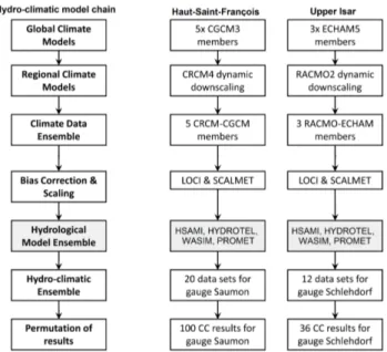
2.2 The hydro-climatic model chain
Figure 2 illustrates the chain of models used to generate the flow simulations. This chain consists of an ensemble of cli-mate simulations feeding an ensemble of hydrological mod-els of various structural complexities. The upper half of the diagram in Fig. 2 depicts the two climate data ensembles used in the study while the lower part represents the hydro-logical ensemble and the associated scaling and bias correc-tion tools required to adjust the climate model data to the hydrological models. These tools connect the top and bottom parts. The combination of climate and hydrological models generates the hydro-climatic ensemble that is analysed to quantify the contribution to uncertainty induced by the hy-drological models with respect to the climate natural vari-ability estimated from the climate models.
2.2.1 The climate simulation ensemble
Fig. 1.Location ofau SaumonandSchlehdorf catchments.
Fig. 2.The hydro-climatic model chain.
This natural variability can be estimated by repeating a cli-mate change experiment using a given GCM several times when only the initial conditions are changed by small pertur-bations (Murphy et al., 2009; Braun et al., 2012). Although the natural variability is just a fraction of the total climate simulations uncertainty, it is irreducible even if perfect mod-els would be available. Therefore, natural variability is used in this study to compare the significance of the uncertainty induced by the hydrological models compared to the irre-ducible baseline uncertainty.
Driving hydrological models of different structural com-plexity over small, heterogeneous catchments with an en-semble of climate scenarios requires further (statistical) ad-justment to the forcing variables in order to suit the hydro-logical modelling scale (e.g., 1×1 km2). A post-processing is applied to correct biases in RCM temperature and pre-cipitation before downscaling the fields to the hydrological model scale. Monthly correction factors are computed based
on the difference between the ensemble-mean of the 30-yr mean monthly minimum and maximum air temperature for the reference period and the 30-yr monthly means of daily-observed minimum and maximum air temperature. The cor-rection is then applied to each member of the ensemble to conserve the inter-member variance used to estimate the nat-ural variability.
The resulting seasonal climate change signals from the cli-mate simulations ensemble (after bias correction and down-scaling) are presented in Fig. 3 for both catchments. The mean annual projected change in air temperature for theHaut
Saint-Franc¸oisarea between the reference and future period
is about 3.0◦
C. However, the winter months (December to February, DJF) show a stronger warming and a stronger inter-member variability. The average change in precipitation is positive for all seasons but summer (JJA). In the Upper Isar region annual warming is estimated to be 2.2◦
Fig. 3.Climate change signals overHaut-Saint-Franc¸ois(left) and Upper Isar (right) regions.
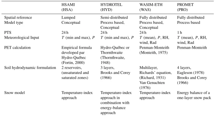
2.2.2 The hydrological model ensemble
An ensemble of four hydrological models displaying a range of structural complexity has been constructed. The mod-els range from lumped and conceptual to fully distributed and physically based. Both spatial and temporal resolutions differ within the hydrological model ensemble. The model HSAMI (HSA; Bisson and Roberge, 1983; Fortin, 2000) is a conceptual and lumped model that uses a set of param-eters to describe the entire catchment. The conceptual and process-based semi-distributed model HYDROTEL (HYD; Fortin et al., 2001; Turcotte et al., 2003) defines a drainage structure based on unitary catchment units and derives be-havioural information for each RHHU (relatively homoge-nous hydrological units). The conceptual and process-based fully-distributed model WASIM-ETH (WAS; Schulla and Jasper, 2007) and the process-based and fully distributed model PROMET (PRO; Mauser and Sch¨adlich, 1998) are distributed on a grid with a mesh of 1 km. The temporal reso-lution for all hydrological models is daily with the exception of PROMET that requires hourly forcing. PROMET simu-lation results are, thus, aggregated to daily means after the simulation is completed. Table 1 presents the characteristics of each of the hydrological models.
Meteorological inputs were processed to fit each model’s potential evapotranspiration formulation requirements. For
theau Saumoncatchment, HSAMI and HYDROTEL use the
empirical formulation developed by Hydro-Qu´ebec (Fortin, 2000). For Bavaria, HSAMI uses the Hydro-Qu´ebec for-mulation while the Thornthwaite forfor-mulation (Thornth-waite, 1948) is used in HYDROTEL. Both formulations use daily minimum and maximum temperatures. WASIM and PROMET use the Penman-Monteith equation which re-quires additional meteorological inputs for relative humidity, wind speed and net radiation. The soil hydrodynamic for-mulation is also different within the ensemble. In HSAMI, vertical flows in the soil column are represented by two conceptual and linear reservoirs that represent the unsatu-rated and satuunsatu-rated zones, while HYDROTEL, WASIM and PROMET compute soil water fluxes and storage with param-eters adjusted to different soil layers. HYDROTEL provides
a lumped characterisation of soils at the subcatchment scale and considers the soil column properties as being vertically homogenous.
The computation of snow accumulation and melting is also treated differently in each model; the snow pack evolution in PROMET respects the energy balance in the snow pack, while the other models use simpler temperature-index ap-proaches.
In all four hydrological models, calibration has been made on the 1990–1999 period. In order to evaluate the predictive capacity of each hydrological model, a simple split sample test has been applied using the 1975–1989 period for valida-tion. Automatic calibration is applied for HSAMI and HY-DROTEL by using the Shuffled Complex Evolution optimi-sation method (Duan, 2003) with the sum of squared errors between observed and simulated runoff as objective func-tion. WASIM is manually calibrated by adjustment of land use specific minimal resistance parameters for evapotranspi-ration and four recession parameters for runoff. PROMET is calibrated by changing the soil parameters.
The Nash-Sutcliffe (1970) efficiency coefficient (NS) is computed in order to evaluate the performance of the hy-drological models (Table 2). For the validation period in the
au Saumoncatchment, the daily NS has values of about 0.6
for all models, with the exception of PRO, which achieves a value of 0.2. In the Schlehdorf catchment, the daily N.S has values of 0.75 for HSA and HYD, but for PRO it is only 0.12. Despite the low performance of PRO for daily NS, it has a comparable performance in the evaluation of hydrolog-ical indicators on the reference period (see Sect. 3.1). Cali-bration and validation processes are more widely described in Ludwig et al. (2012).
2.3 Hydrological indicators
The analysis of the impact of climate change on hydrology is evaluated on the following four hydrological indicators:
1. The overall mean flow (OMF), defined as the mean daily runoff over the entire period of the investigated time se-ries.
2. The 2-yr return period 7-day low flow (7LF2), calcu-lated from a 7-day moving average applied on daily runoff data. The lowest value over a year is kept as the yearly low flow. A statistical distribution is fitted to the series of yearly low flows to compute the low flow that occurs statistically every 2 yr (DVWK, 1983).
Table 1.Characteristics of the hydrological model ensemble.
HSAMI HYDROTEL WASIM-ETH PROMET
(HSA) (HYD) (WAS) (PRO)
Spatial reference Lumped Semi-distributed Fully distributed Fully distributed
Model type Conceptual Process based, Process based, Process based
Conceptual Conceptual
PTS 24 h 24 h 24 h 1 h
Meteorological Input T (min and max),P T (min and max),P T (mean),P, RH, T (mean),P, RH,
wind, Rad wind, Rad
PET calculation Empirical formula Hydro-Qu´ebec or Penman-Monteith Penman-Monteith
developed par Thornthwaite (Monteith, 1975)
Hydro-Qu´ebec (Thornthwaite,
(Fortin, 2000) 1948)
Soil hydrodynamic formulation 2 reservoirs, 3 layers, Multilayer, 4 layers,
(unsaturated and Brooks and Corey Richards’ equation, Eagleson (1978)
saturated zones) (1966) (Richard, 1931) Brooks and Corey
Van Genuchten (1966)
(1976)
Snow model Temperature-index Temperature-index Temperature-index Energy balance of a
approach approach in approach one-layer snow pack
combination with energy-balance approach
Note:P(precipitation), PET (potential evapotranspiration), PTS (processing time step), Rad (radiation), RH (relative humidity) andT(temperature).
Table 2.Daily Nash-Sutcliffe efficiency coefficient (NS) for the
cal-ibration (1990–1999) and validation (1975–1989) periods.
HSA HYD WAS PRO
Cal. Val. Cal. Val. Cal. Val. Cal. Val.
au Saumon 0.74 0.67 0.60 0.64 0.48 0.60 0.37 0.20 Schlehdorf 0.83 0.75 0.80 0.76 0.87 0.82 0.34 0.12
To calculate 7LF2 and HF2, it is assumed that the time series follow the log Pearson III probability density function, following the German Association of Water (DVWK, 1979, 1983).
4. The Julian day of spring-flood half volume (JDSF) iden-tifies the date over the hydrological year at which half of the total volume of water has been discharged at the gauging station (Bourdillon et al., 2011). This indicator targets the spring flood peak, from February to June in Qu´ebec and from March to July in Bavaria.
Both catchments show an important annual cycle in the hy-drological regime. Two distinct periods representing summer and winter are, therefore, defined for the analysis. For the Qu´ebec catchment, the summer covers the period from June to November and the winter covers December to May while in Bavaria the summer goes from March to August and the winter from September to February.
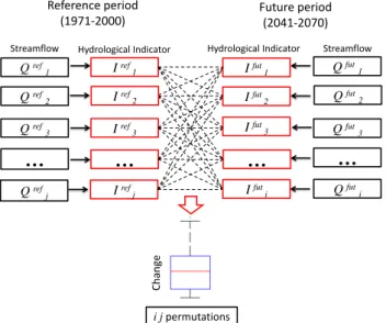
2.4 Permutations and statistical test
At the very end of the modelling chain (Fig. 2), the present and future climatological values of the hydrological indica-tors are permuted across members to increase the sample of our climate change signals dataset (e.g., Bourdillon et al., 2011). This operation is based on the assumption that each member is considered as an independent realisation of cli-mate, both in the reference and the future periods. With per-mutation, the future of a given member is not only com-pared with the present of the same member, but also with the present of all other members. For instance, five GCM mem-bers used in a single branch of the modelling chain (i.e., used to drive only one RCM and one hydrological model) produce five present and five future hydrological outputs. With per-mutation, 25 future versus present differences are obtained for the hydrological indicators, as shown in Fig. 4. There-fore, using the permutations, 25 values of relative differences are obtained with five reference and five future hydrologi-cal indicators at theau Saumoncatchment. ForSchlehdorf, nine values are obtained with the three-member ECHAM5 ensemble. The median of the change values gives the climate change signal while the variability gives an estimation of the uncertainty associated to that signal.
Q ref
1 I ref 1 Q ref
2
Q ref
3 I ref 3
…
…
Q ref
j I
ref j
Q fut 1
Q fut 2
Q fut 3
Q fut i I fut
1
I fut 2
I fut 3
…
I futi Reference period
(1971-2000)
Future period (2041-2070)
Ch
an
ge
Streamflow Hydrological Indicator Hydrological Indicator Streamflow
…
i j permutations I ref
2
Fig. 4.Schematic representation of the permutation process.
with equal medians, against the alternative that they do not have equal medians (Wilks, 2006). For instance, for a given hydrological indicator (e.g., OMF), we have four climate change signal samples, which have been obtained with the four different hydrological models. The Wilcoxon rank-sum test tells us, if two samples, obtained from two distinct mod-els (e.g., HSAMI and HYDROTEL), are independent or not (see Sect. 3.3). It should be noted that the climate change sig-nals from the same model are considered as independent, as they come from independent climate simulations.
3 Results and discussion
The aim of the present study is to assess the contribution of hydrological models to uncertainty in the climate change sig-nal for water resources management. First, the performance of the hydrological models is evaluated over the reference pe-riod by validating the simulated indicators when the model is forced with station data against the observed flow at the gauging station. The differences from observations are used to assess the performance of the hydrological model ensem-ble (Sect. 3.1). Second, the impact of forcing the hydrolog-ical models with the climate model projections is assessed through the hydro-climatic simulations using the ensemble of calibrated hydrological models forced by the ensemble of cli-mate simulations (Sect. 3.2). Finally, the relative difference in the hydrological indicators between the reference (1971– 2000) and future (2041–2070) periods is calculated to eval-uate the climate change signals. A statistical test is used for all given indicators in order to compare the series of relative change of hydrological indicators obtained with the different hydrological models.
Fig. 5.Performance of the hydrological models over the reference
period. The left panels show the relative error as computed with Eq. (1), while the right panels show the absolute error in m3s−1or days.
3.1 Performance of the hydrological models
In order to evaluate the hydrological models when forced by observed station data, the simulated hydrological indicators are compared to the hydrological indicators computed from the gauging station data for both catchments. Figure 5 (left) shows relative errorsEi between indicators computed from
simulations and from observed flows as computed following Eq. (1):
Ei=
I(sim)i−I(obs) I(obs)
(1)
where,I(obs)is the value of the indicator as computed from
observed flows;I(sim)i is the indicator calculated from the
simulated flows with the hydrological model i forced by stations data over the validation period. The right panels in Fig. 5 show the absolute error (in m3s−1or days for JDSF).
Errors related to the OMF over the whole period are rela-tively small for both catchments (less than 10 %). The hydro-logical models underestimate the OMF for the au Saumon
is small. For instance, forau Saumon, HYD, PRO and WAS have a mean error of 23 % in 7LF2-SUMMER, which repre-sents only 0.3 m3s−1. HSA presents a large relative error for this indicator (about 260 %) which reaches 3.4 m3s−1. Over
Schlehdorf, the more complex and physically based model
PRO that could be thought to better handle low flows show similar performance as the others models in 7LF2-WINTER. For high flows, WAS and PRO have small relative er-rors forau Saumonbut these small relative errors can rep-resent a large amount of water as it can be seen in the right panel of Fig. 5. ForSchlehdorf, the best performance in HF2-SUMMER is obtained with WAS while PRO has the largest deviation.
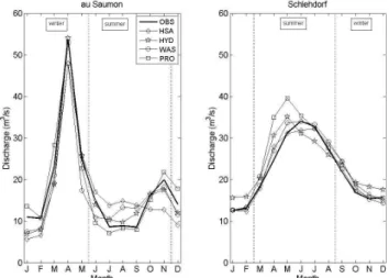
Figure 6 shows the observed and simulated (with the hy-drological models forced by meteorological station data) mean hydrographs. Au Saumon presents two high-flow events. The first one in spring (driven by snowmelt) is well simulated by HYD and PRO, but underestimated by HSA and WAS. A second but smaller high-flow event occurs in summer (driven by rain) which is not captured by HSA. The
au Saumon summer low flows are overestimated by HSA
and WAS.Schlehdorf is characterised by one summer peak-flow which results from both snowmelt and precipitation. The peak is overestimated by PRO and is simulated earlier by most hydrological models.Schlehdorf winter low flows are overestimated by HYD.
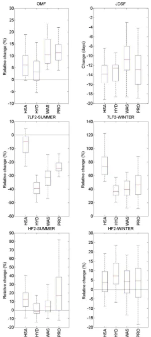
3.2 Climate change impact on water resources
Figures 7 and 8 show the impact of climate change on hydro-logical indicators forau SaumonandSchlehdorfcatchments, respectively. The change is expressed as differences of simu-lated hydrological indicators (1Iij)from the reference (Ijref)
to the future period (Iifut).
1Iij=
Iifut−Ijref
Ijref (2)
whereiandjrepresent the member of the climate simulation from which the hydrological indicator was taken. For each hydrological model, the boxplots present the change values obtained by the permutations (25 values for each boxplot at
au Saumonand 9 values atSchlehdorf as seen in Fig. 4). In
both figures, the change of each hydrological indicator (fol-lowing Eq. 2) is shown. The two extreme indicators 7LF2 and HF2 are calculated for the two seasons (summer and winter). The change in JDSF is only expressed as the absolute differ-ence between the present and future values in days.
In Fig. 7, the hydro-climatic ensemble suggests a general increase in the overall mean flow forau Saumon.The change of the OMF median values varies between 3 % and 11 % for the different hydrological models. The extremes of the ex-pected changes range between−6 % and 22 %. The whole
hydro-climatic ensemble predicts an earlier spring flood. The median change value of the JDSF varies from−11 to−13
Fig. 6.Observed and simulated (forced by stations data)
hydro-graphs forau SaumonandSchlehdorf over the reference period.
days, while the overall range goes from −3 to −19 days. The increase in temperature projected by the climate mod-els (Fig. 2) simulates an earlier melt in the future simulated snow cover. The change in the low flow indicators depicts a larger variability between the hydrological models. For the 7LF2-SUMMER, the median change values vary from
−5 % to−40 %. The reduction in the precipitation and the
increase of the potential evapotranspiration (PET not shown) explain this overall decrease in SUMMER. For 7LF2-WINTER, HSA has a significantly larger median change value (+70 %), while the other three models show values of about +40 %. The change in the summer high flow in-dicator (HF2-SUMMER) ranges from−3 % to 18 %. PRO is more sensitive to the range in climate forcing and shows the largest spread in the indicator from−10 % to+80 %. The median change values of HF2-WINTER are around +5 % with a range from−18 % to+23. The overall trend shows an increase in high flows.
Schlehdorf (Fig. 8) shows a general, but smaller
diminu-tion of the OMF, the median change value varies between
−1 % and−6 %. The spring flood discharge happens sooner
in the simulations with the median difference ranging be-tween−4 and −6 days. The median of summer low flow
Fig. 7.Changes of hydrological indicators from reference to future period atau Saumon(Haut St-Franc¸ois, Qu´ebec) of overall mean flow (OMF), the Julian day of spring-flood half volume (JDSF), the 2-yr return period 7-day low flow (7LF2) in summer and winter, and the 2-yr return period high flow (HF2) in summer and winter. For each hydrological indicator, the relative change (as calculated with Eq. 2) is presented. On each box, the central mark is the median, the edges of the box are the 25th and 75th percentiles, and the whiskers extend to the most extreme value.
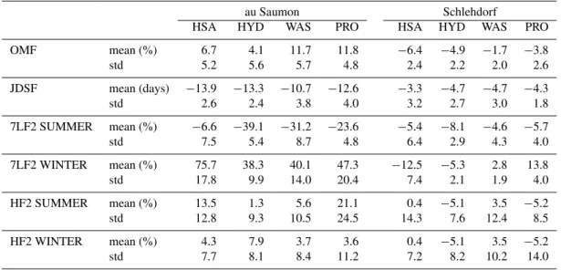
relative difference (median of−5 %), while the other mod-els show a median value of about +3 %. The total change in HF2-WINTER ranges between−8 % and+30 % where a general increase in high flows is expected for all hydrologi-cal models but HSA. Table 3 shows the mean and standard deviation (std) from the relative change series presented in Figs. 7 and 8.
Fig. 8.Same as Fig. 7 but forSchlehdorf.
3.3 Hydrological models contribution to uncertainty
Table 3.Mean and standard deviation (std) from the change series presented in Figs. 7 and 8.
au Saumon Schlehdorf
HSA HYD WAS PRO HSA HYD WAS PRO
OMF mean (%) 6.7 4.1 11.7 11.8 −6.4 −4.9 −1.7 −3.8
std 5.2 5.6 5.7 4.8 2.4 2.2 2.0 2.6
JDSF mean (days) −13.9 −13.3 −10.7 −12.6 −3.3 −4.7 −4.7 −4.3
std 2.6 2.4 3.8 4.0 3.2 2.7 3.0 1.8
7LF2 SUMMER mean (%) −6.6 −39.1 −31.2 −23.6 −5.4 −8.1 −4.6 −5.7
std 7.5 5.4 8.7 4.8 6.4 2.9 4.3 4.0
7LF2 WINTER mean (%) 75.7 38.3 40.1 47.3 −12.5 −5.3 2.8 13.8
std 17.8 9.9 14.0 20.4 7.4 2.1 1.9 4.0
HF2 SUMMER mean (%) 13.5 1.3 5.6 21.1 0.4 −5.1 3.5 −5.2
std 12.8 9.3 10.5 24.5 14.3 7.6 12.4 8.5
HF2 WINTER mean (%) 4.3 7.9 3.7 3.6 0.4 −5.1 3.5 −5.2
std 7.7 8.1 8.4 11.2 7.2 8.2 10.2 14.0
The rank-sum Wilcoxon test is used in order to compare pairs of climate change signal ensemble obtained from two distinct hydrological models. For each hydrological indica-tor, we evaluated if two samples (one sample from each hy-drological model) have been drawn from the same distribu-tion (the null hypothesis) with a significance level of 5 %. If the null hypothesis is not rejected, it could be an indication that the climate change signals from two hydrological mod-els provide similar information. Note that this does not verify the null hypothesis, but only says that it cannot be rejected from the available information. This test was applied to the relative differences (except for JDSF where it was applied to absolute differences in days), as specified in Figs. 7 and 8.
The Wilcoxon test results are shown in Table 4 for au
SaumonandSchlehdorf where the series of climate change
impact on hydrological indicators are compared for all the pairs of models. The OMF atau Saumon, the null hypothe-sis is not rejected when comparing the pairs HSA-HYD, and WAS-PRO. For OMF Schlehdorf, the only pairs of model that lead to rejection are WAS-HSA and WAS-HYD. The large difference in the Wilcoxon test results over the two catchments might originate from the formulation of potential evapotranspiration (PET); PRO and WAS use the complex Penman-Monteith while HYD and HSA use temperature-based empirical approaches. However, the model pairs HSA-PRO and HYD-HSA-PRO do not reject the null hypothesis for
Schlehdorf.Bormann (2011) reported that different PET
for-mulations following different approaches show significantly different sensitivities to climate change.
The change in the JDSF is similarly predicted with all hydrological models overSchlehdorf.Over theau Saumon, only WAS behaves differently to the less complex HSA and HYD. So in this case the signal is more robust because this indicator depends mostly on temperature.
The low flow shows greater differences between models. The season when low flows are most severe is different; it happens in summer forau Saumon and in winter for
Schle-hdorf. In au Saumon, the null hypothesis is rejected for all
models pairs for the 7LF2-SUMMER, but it is the concep-tual model HSA which presents the largest difference with all other models (see Fig. 7). InSchlehdorf the null hypothesis for 7LF2-WINTER is rejected for all model pairs except for the pair HSA-HYD. However, a very different behaviour is shown between lumped and distributed models for low flows. The lumped and semi-distributed models predict a negative change, while the fully distributed models predict a positive change (Fig. 8). TheSchlehdorfcatchment is very steep and this could affect the baseflow simulation, which is better rep-resented in the semi-distributed and fully distributed models. In the less severe low flow periods (winter forau Saumon, and summer forSchlehdorf), groundwater recharge is larger, so this leads to a more stable baseflow and smaller differ-ences in the simulated low-flow quantities between hydro-logical models. These differences may also be influenced by the PET formulation.
The highest flows are seen in winter forau Saumonand in summer forSchlehdorf. The null hypothesis is not rejected when comparing all pairs of hydrological models for the HF2 in these periods. However, a large uncertainty is present in this indicator, but it is more related to the natural variability simulated by climate models than to choice of the hydrologi-cal model (Figs. 7 and 8). Nevertheless, the choice of the hy-drological model affects the HF2-SUMMER inau Saumon.
Table 4.Results of Wilcoxon test comparing pairs of hydrological models for (a)au Saumon, and (b)Schlehdorf.The p-value is shown and the shaded area indicates a rejection of the null hypothesis at significance level of 5 %.
(a) au Saumon HSA-HYD HSA-PRO HSA-WAS HYD-PRO HYD-WAS PRO-WAS
OMF 0.140 0.001 0.003 <0.001 <0.001 0.816
JDSF 0.421 0.362 0.003 0.641 0.008 0.064
7LF2 SUMMER <0.001 <0.001 <0.001 <0.001 0.001 0.001
7LF2 WINTER <0.001 <0.001 <0.001 0.107 0.641 0.237
HF2 SUMMER 0.001 0.449 0.020 0.002 0.222 0.024
HF2 WINTER 0.130 0.923 0.954 0.200 0.107 0.938
(b) Schlehdorf HSA-HYD HSA-PRO HSA-WAS HYD-PRO HYD-WAS PRO-WAS
OMF 0.297 0.063 0.001 0.436 0.006 0.094
JDSF 0.241 0.372 0.248 0.422 0.879 0.423
7LF2 SUMMER 0.258 0.730 0.931 0.258 0.077 0.730
7LF2 WINTER 0.077 <0.001 <0.001 <0.001 <0.001 <0.001
HF2 SUMMER 0.340 0.436 0.863 0.863 0.094 0.113
HF2 WINTER 0.0503 0.063 0.0503 0.666 0.730 >0.999
use of a hydrological model ensemble would, thus, be rec-ommended in order to fully assess the uncertainty on hy-drological indicators due to climate change. ForSchlehdorf, only OMF and 7LF2 seem to be sensitive to the selection of hydrological model. To analyse the high-flow indicator or springflood timing indicator, the recommendation to use a simple conceptual model can be made with a certain level of confidence. Another important aspect is that the analysis of the uncertainty from the hydrological models cannot be transferred from site to site and seems to have to be repeated for every catchment. A regional analysis would be required to see if the conclusions present a regional behaviour.
4 Discussion and conclusions
The present study looked at the uncertainty in projecting fu-ture changes in runoff characteristics induced by the choice of hydrological models for two distinct natural flow catch-ments. A hydro-climatic ensemble is constructed with a com-bination of an ensemble of climate scenarios and an ensem-ble of hydrological models. The major strength of the climatic ensemble approach is that the ability of the hydro-logical models to reproduce hydrohydro-logical characteristics can be compared and the uncertainty of future changes in runoff behaviour can be assessed. Although the selected models in our study cover a wide range of complexity, a limitation of this approach is that the selection of hydrological models will never cover the full space of plausible models and conceptu-alisations. By not including some plausible models that are substantially different from the selected models, can result in underestimated model uncertainty. A complete evaluation of this component of the uncertainty in hydrological projections represents a research challenge (Refsgaard et al., 2012).
In this study, four hydrological models have been chosen from those used in scientific or administrative assessment
of climate change impacts on river runoff in Qu´ebec and Bavaria. The complexity of these models ranges from con-ceptual and lumped to process-based and fully distributed.
The principal objective of the paper is to assess the con-tribution of hydrological models’ uncertainty in the climate change signal for water resources management. The results of our study suggest that the added value depends on the hy-drological indicator considered and on the region of interest. Regarding hydrological indicators, Bl¨oschl and Monta-nari (2010) suggest that that we can have reasonable con-fidence in predicting hydrological changes that are mainly driven by air temperature (e.g., snowmelt and low flows through evapotranspiration) as opposed to rainfall-driven events like floods. Similarly, Bo´e et al. (2009) have more confidence to projected changes of low and mean flows. Our results suggest that not only the forcing climate variables, but also the hydrological model plays a key role in the un-certainty of projected climate change signal of hydrological indicators.
In the case of high flows, most of the hydrological mod-els lead to comparable results; therefore, both lumped and distributed models can be used.
The largest relative difference between hydrological model outputs is seen in changes in low flow. However, it is important to remember that the hydrological models used in this study were not specifically calibrated for low flows, which is reflected in the results for the reference period. Thus, the differences are not only influenced by the model structure itself, but also by the calibration (e.g., Maurer et al., 2010), and this issue should be evaluated by using a similar calibration strategy for all models.
The results of this study support that the simulation of low flows is an important challenge and need to be improved for low flow management, both in present-day climate and in a perturbed climate (Pushpalatha et al., 2009). Therefore, one must be cautious in the evaluation of climate change impacts on low-flow conditions from a single model (e.g., Bae et al., 2011). Our study confirms the results of recent studies by Maurer et al. (2010), who found that hydrological model selection will be a significant factor in assessing pro-jected changes to low flows, and by Najafi et al. (2011) and Vansteenkiste et al. (2012), who showed that the uncertainty associated with the hydrological models becomes larger for dry periods.
The GCM is reported to be the most important source of uncertainty in hydrologic climate change impact studies (e.g., Graham et al., 2007; Wilby and Harris, 2006). How-ever, we should still quantify and estimate the uncertainties generated by hydrological modelling. Translation of uncer-tainty into future risks can provide a valuable contribution to the decision-making process (Beven, 2001). Furthermore, it is necessary to better understand hydrological processes in present climate (e.g., the surface-groundwater interactions to simulate low flows) in order to understand how a changed climate will affect future water resources availability.
All in all, we suggest that the uncertainty in projec-tions added by the hydrological models should be included in climate change impact studies, especially for the anal-ysis of mean and low flows. In the absence of an ac-ceptance/rejection criterion (Beven, 2007), all hydrological models should be considered equally accurate and, therefore, should equally contribute to the quantification of the uncer-tainty. The generalisation of this conclusion would require application to more sites and should include other sources of uncertainty (e.g., calibration of hydrological models or use of different GCMs and RCMs).
Another interesting approach is the use of a multimodel ensemble to assess structural uncertainties, which has been done by Seiller et al. (2012) to evaluate the relevance of twenty lumped conceptual hydrological models in a climate change context. Results show that using a single model may provide hazardous results when the model is to be applied in contrasted conditions, and generally the twenty-model en-semble gives a better performance.
Acknowledgements. The authors acknowledge the fruitful revisions of P. Willems and an anonymous reviewer. Editor (H. Madsen) is also thanked for his constructive comments. The CRCM data has been generated and supplied by Ouranos. The authors thank E. van Meijgaard (KNMI) for his invaluable support in acquiring the RACMO data. Financial support for the undertaking of this work has been provided by the Ouranos’ FRSCO (Fonds de recherche en sciences du climat d’Ouranos) programme, the PSR-SIIRI Qu´ebec MDEIE programme, and by the Bavarian Environment Agency (LfU). Thanks to F. Anctil for the valuable discussion of this paper.
Edited by: H. Madsen
References
Bae, D.-H., Jung, I.-W., and Lettenmaier, D. P.: Hydrologic uncer-tainties in climate change from IPCC AR4 GCM simulations of the Chungju Basin, Korea, J. Hydrol., 401, 90–105, 2011. Beven, K.: Rainfall-Runoff modelling, The primer, John Wiley &
Sons Ltd., West Sussex, England, 2001.
Beven, K.: Towards integrated environmental models of every-where: uncertainty, data and modelling as a learning process, Hydrol. Earth Syst. Sci., 11, 460–467, doi:10.5194/hess-11-460-2007, 2007.
Bisson, J. L. and Roberge, F.: Pr´evisions des apports naturels: exp´erience d’Hydro-Qu´ebec, in: Proc., Workshop on Flow Pre-dictions, Institute of Electrical and Electronics Engineers IEEE, Toronto, Canada, November 1983.
Bl¨oschl, G. and Montanari, A.: Climate change impacts – throwing the dice?, Hydrol. Process., 24, 374–381, doi:10.1002/hyp.7574, 2010.
Bo´e, J., Terray, L., Martin, E., and Habets, F.: Projected changes in components of the hydrological cycle in French river basins during the 21st century, Water Resour. Res., 45, W08426, doi:10.1029/2008WR007437, 2009.
Bormann, H.: Sensitivity analysis of 18 different potential evapotranspiration models to observed climatic change at German climate stations, Climatic Change, 104, 729–753, doi:10.1007/s10584-010-9869-7, 2011.
Bourdillon, R., Ricard, S., Roussel, D., Turcotte, R., and Cyr, J. F.: ´
Evaluer, `a l’horizon 2050, les impacts pour le Qu´ebec m´eridional sur les ´ecoulements en eau, en excluant l’effet de la gestion des barrages, sur des indicateurs hydrologiques utilis´es en gestion de l’eau. ´Etat des connaissances au 31 mars 2011, Rapport interne au Centre d’expertise hydrique du Qu´ebec (CEHQ), Qu´ebec, Canada, 72 pp. + annexes, 2011.
Braun, M., Caya, D., Frigon, A., and Slivitzky, M.: Internal Vari-ability of Canadian RCM’s Hydrological Variables at the Basin Scale in Quebec and Labrador, J. Hydrometeorol., 13, 443–462, 2012.
Brooks, R. H. and Corey, A. T.: Properties of porous media affecting fluid flow, J. Irrig. Drain. Eng.-ASCE, 92, 61–88, 1966. Chen, J., Brissette, F. P., and Leconte, R.: Uncertainty of
downscaling method in quantifying the impact of cli-mate change on hydrology, J. Hydrol., 401, 190–202, doi:10.1016/j.jhydrol.2011.02.020, 2011.
of this century, Climatic Change, 81, 7–30, doi:10.1007/s10584-006-9210-7, 2007.
Crosbie, R. S., Dawes, W. R., Charles, S. P., Mpelasoka, F. S., Aryal, S., Barron, O., and Summerell, G. K.: Differences in future recharge estimates due to GCMs, downscaling meth-ods and hydrological models, Geophys. Res. Lett., 38, L11406, doi:10.1029/2011gl047657, 2011.
de El´ıa, R. and Cˆot´e, H.: Climate and climate change sensitivity to model configuration in the Canadian RCM over North America, Meteorol. Z., 19, 325–339, doi:10.1127/0941-2948/2010/0469, 2010.
D´equ´e, M., Rowell, D., L¨uthi, D., Giorgi, F., Christensen, J., Rockel, B., Jacob, D., Kjellstr¨om, E., de Castro, M., and van den Hurk, B.: An intercomparison of regional climate simulations for Europe: assessing uncertainties in model projections, Climatic Change, 81, 53–70, doi:10.1007/s10584-006-9228-x, 2007. Dibike, Y. B. and Coulibaly, P.: Hydrologic impact of climate
change in the Saguenay watershed: comparison of downscal-ing methods and hydrologic models, J. Hydrol., 307, 145–163, doi:10.1016/j.jhydrol.2004.10.012, 2005.
Duan, Q: Global Optimization for Watershed Model Calibration, in: Calibration of Watershed Models, edited by: Duan, Q., Gupta, H., Sorooshian, S., Rousseau, A., and Turcotte, R., Water Science and Application, Vol. 6, American Geophysical Union, Washing-ton, USA, 89–104, 2003.
DVWK: Empfehlung zur Berechnung der Hochwasserwahrschein-lichkeit. DVWK-Regeln zur Wasserwirtschaft, Verlag Paul Parey, Hamburg, Berlin, 1979.
DVWK: Niedrigwasseranalyse Teil I: Statistische Untersuchung des Niedrigwasser-Abflusses, Verlag Paul Parey, Hamburg und Berlin, 1983.
Eagleson, P. S.: Climate, soil, and vegetation: 3. A simplified model of soil moisture movement in the liquid phase, Water Resour. Res., 14, 722–730, doi:10.1029/WR014i005p00722, 1978. Foley, A. M.: Uncertainty in regional climate
mod-elling: A review, Prog. Physi. Geogr., 34, 647–670, doi:10.1177/0309133310375654, 2010.
Fortin, J. P., Turcotte, R., Massicotte, S., Moussa, R., Fitzback, J., and Villeneuve, J. P.: Distributed watershed model compatible with remote sensing and GIS data, I: description of model, J. Hydrol. Eng., 6, 91–99, 2001.
Fortin, V.: Le mod`ele m´et´eo-apport HSAMI: historique, th´eorie et application, Institut de recherche d’Hydro-Qu´ebec (IREQ), Varennes, 68 pp., 2000.
Gosling, S. N., Taylor, R. G., Arnell, N. W., and Todd, M. C.: A comparative analysis of projected impacts of climate change on river runoff from global and catchment-scale hydrological mod-els, Hydrol. Earth Syst. Sci., 15, 279–294, doi:10.5194/hess-15-279-2011, 2011.
Graham, L. P., Hagemann, S., Jaun, S., and Beniston, M.: On inter-preting hydrological change from regional climate models, Cli-matic Change, 81, 97–122, 2007.
Hawkins, E. and Sutton, R.: The potential to narrow uncertainty in regional climate predictions, B. Am. Meteorol. Soc., 90, 1095– 1107, 2009.
Horton, P., Schaefli, B., Mezghani, A., Hingray, B., and Musy, A.: Assessment of climate-change impacts on alpine discharge regimes with climate model uncertainty, Hydrol. Process., 20, 2091–2109, doi:10.1002/hyp.6197, 2006.
Jiang, T., Chen, Y. D., Xu, C.-Y., Chen, X. H., Chen, X., and Singh, V. P.: Comparison of hydrological impacts of climate change simulated by six hydrological models in the Dongjiang Basin, South China, J. Hydrol., 336, 316–333, 2007.
Jones, R. N., Chiew, F. H. S., Boughton, W. C., and Zhang, L.: Esti-mating the sensitivity of mean annual runoff to climate change using selected hydrological models, Adv. Water Resour., 29, 1419–1429, 2006.
Kay, A. L., Davies, H. N., Bell, V. A., and Jones, R. G.: Compari-son of uncertainty sources for climate change impacts: flood fre-quency in England, Climatic Change, 92, 41–63, 2009. Ludwig, R., May, I., Turcotte, R., Vescovi, L., Braun, M., Cyr,
J.-F., Fortin, L.-G., Chaumont, D., Biner, S., Chartier, I., Caya, D., and Mauser, W.: The role of hydrological model complexity and uncertainty in climate change impact assessment, Adv. Geosci., 21, 63–71, doi:10.5194/adgeo-21-63-2009, 2009.
Ludwig, R., Turcotte, R., Chaumont, D., and Caya, D.: Adapting re-gional watershed management under climate change conditions – a perspective from the QBIC3project, Adv. Geosci., in prepa-ration, 2013.
Marke, T.: Development and application of a model interface to couple land surface models with regional climate models for climate change risk assessment in the Upper Danube wa-tershed, Fakult¨at f¨ur Geowissenschaften, Ludwig-Maximilians-Universit¨at, M¨unchen, 2008.
Maurer, E. P., Brekke, L. D., and Pruitt, T.: Contrasting lumped and distributed hydrology models for estimating climate change im-pacts on California watersheds, J. Am. Water Resour. As., 46, 1024–1035, 2010.
Mauser, W. and Bach, H.: PROMET – Large scale distributed hy-drological modelling to study the impact of climate change on the water flows of mountain watersheds, J. Hydrol., 376, 362– 377, doi:10.1016/j.jhydrol.2009.07.046, 2009.
Mauser, W. and Sch¨adlich, S.: Modelling the spatial distribution of evapotranspiration on different scales using remote sens-ing data, J. Hydrol., 212–213, 250–267, doi:10.1016/s0022-1694(98)00228-5, 1998.
Monteith, J. L.: Vegetation and the Atmosphere, Vol. 1, Principles, Elsevier, New York, 1975.
Muerth, M. J., Gauvin St-Denis, B., Ricard, S., Vel´azquez, J. A., Schmid, J., Minville, M., Caya, D., Chaumont, D., Ludwig, R., and Turcotte, R.: On the need for bias correction in re-gional climate scenarios to assess climate change impacts on river runoff, Hydrol. Earth Syst. Sci. Discuss., 9, 10205–10243, doi:10.5194/hessd-9-10205-2012, 2012.
Murphy, J. M., Sexton, D. M. H., Jenkins, G. J., Booth, B. B. B., Brown, C. C., Clark, R. T., Collins, M., Harris, G. R., Kendon, E. J., Betts, R. A., Brown, S. J., Humphrey, K. A., McCarthy, M. P., McDonald, R. E., Stephens, A., Wallace, C., Warren, R., Wilby, R., and Wood, R. A.: UK Climate Projections Science Report: Climate change projections, Met Office Hadley Centre, Exeter, UK, 192 pp., 2009.
Najafi, M. R., Moradkhani, H., and Jung, I. W.: Assessing the uncer-tainties of hydrologic model selection in climate change impact studies, Hydrol. Process., 25, 2814–2826, 2011.
Poulin, A., Brissette, F., Leconte, R., Arsenault, R., and Maloet, J.-S.: Uncertainty of hydrological modelling in climate change impact studies in a Canadian, snow-dominated river basin, J. Hy-drol., 409, 626–636, 2011.
Prudhomme, C. and Davies, H.: Assessing uncertainties in climate change impact analyses on the river flow regimes in the UK. Part 2: future climate, Climatic Change, 93, 197–222, 2008. Pushpalatha, R., Perrin, C., Le Moine, N., Mathevet, T., and
Andr´eassian, V.: A downward structural sensitivity analysis of hydrological models to improve low-flow simulation, J. Hydrol., 411, 66–76, 2011.
Refsgaard, J. C., Christensen, S., Sonnenborg, T. O., Seifert, D., Højberg, A. L., and Troldborg, L.: Review of strategies for han-dling geological uncertainty in groundwater flow and transport modelling, Adv. Water Resour., 36, 36–50, 2012.
Richards, L. A.: Capillary conduction of liquids through porous mediums, Physics, 1, 318–333, 1931.
Schmidli, J., Frei, C., and Vidale, P. L.: Downscaling from GCM precipitation: a benchmark for dynamical and statis-tical downscaling methods, Int. J. Climatol., 26, 679–689, doi:10.1002/joc.1287, 2006.
Seiller, G., Anctil, F., and Perrin, C.: Multimodel evaluation of twenty lumped hydrological models under contrasted cli-mate conditions, Hydrol. Earth Syst. Sci., 16, 1171–1189, doi:10.5194/hess-16-1171-2012, 2012.
Schulla, J. and Jasper, K.: Model Description WaSiM-ETH, tute for Atmospheric and Climate Science, Swiss Federal Insti-tute of Technology, Z¨urich, 2007.
Teutschbein, C. and Seibert, J.: Regional Climate Models for Hy-drological Impact Studies at the Catchment Scale: A Review of Recent Modeling Strategies, Geography Compass, 4, 834–860, doi:10.1111/j.1749-8198.2010.00357.x, 2010.
Teutschbein, C., Wetterhall, F., and Seibert, J.: Evaluation of dif-ferent downscaling techniques for hydrological climate-change impact studies at the catchment scale, Clim. Dynam., 37, 2087– 2105, doi:10.1007/s00382-010-0979-8, 2011.
Thornthwaite, C. W.: An approach toward a rational classification of climate, Geogr. Rev., 38, 55–94, 1948.
Turcotte, R., Rousseau, A. N., Fortin, J.-P., and Villeneuve, J.-P.: A process-oriented, multiple objective calibration strategy account-ing for model structure, in: Calibration of Watershed Models, edited by: Duan, Q., Gupta, H., Sorooshian, S., Rousseau, A., and Turcotte, R., Water Science and Application, Vol. 6, Ameri-can Geophysical Union, Washington, USA, 153–163, 2003. Van Genuchten, M. T.: A Closed-Form Equation for Predicting the
Hydraulic Conductivity of Unsaturated Soils, Soil Sci. Soc. Am. J., 44, 892–898, 1976.
van Meijgaard, E.: The KNMI regional atmospheric climate model RACMO version 2.1, Koninklijk Nederlands Meteorologisch In-stituut, 2008.
Vansteenkiste, Th., Tavakoli, M., Ntegeka, V., Willems, P., De Smedt, F., and Batelaan, O.: Climate change impact on river flows and catchment hydrology: a comparison of two spatially distributed models, Hydrol. Process., online first: doi:10.1002/hyp.9480, 2012.
Wilby, R. L. and Harris, I.: A framework for assessing uncer-tainties in climate change impacts: Low-flow scenarios for the River Thames, UK, Water Resour. Res., 42, W02419, doi:10.1029/2005wr004065, 2006.
Wilcoxon, F.: Individual Comparisons by Ranking Methods, Bio-metrics Bull., 1, 80–83, 1945.
Wilks, D. S.: Statistical Methods in the Atmospheric Sciences, 2nd Edn., International Geophysics Series, Academic Press, San Diego, CA, 627 pp., 2006.