A Behavioral Analysis Tool for
Models of Software Systems
Universidade Nova de Lisboa Faculdade de Ciências e Tecnologia
Departamento de Informática
Faculdade de Ciências e Tecnologia
Departamento de Informática
Dissertação de Mestrado
Mestrado em Engenharia Informática
A Behavioral Analysis Tool for Models
of Software Systems
Ricardo João Besteiro e Silva (aluno nº 28025)
Faculdade de Ciências e Tecnologia
Departamento de Informática
Dissertação de Mestrado
A Behavioral Analysis Tool for Models of Software Systems
Ricardo João Besteiro e Silva (aluno nº 28025)
Orientador:
Prof. Doutor Luís Caires
Trabalho apresentado no âmbito do Mestrado em Engen-haria Informática, como requisito parcial para obtenção do grau de Mestre em Engenharia Informática.
First and foremost I would like to thank Professor Luís Caires for his support and patience throughout the elaboration of this thesis. I would also like to thank my colleagues Bernardo Toninho and Hugo Vieira for all the times they helped me by providing further insight in the tool they are also familiar with.
Last, but in any means not least, I would like to thank all my friends, family and specially Luísa Lourenço for the not so technical but still important support they provided which made this thesis possible.
Cálculos de processos são linguagens simples que permitem a modelação de sistemas con-correntes de forma a poder ser verificada a sua correcção. É possível usar cálculos de processos para analisar sistemas concorrentes comparando a representação de uma implementação com uma especificação mais geral usando alguma forma de equivalência, ou através da verificação se algumas propriedades descritas numa lógica adequada são verdadeiras.
Bisimulação forte é uma de muitas relações de equivalência definidas para comprar cálculos de processos. Esta relação de equivalência considera processos que têm o mesmo comporta-mento, i.e. realizam as mesmas transições, como equivalentes sem olhar para os detalhes de implementação.
Há vários tipos de lógicas para raciocinar sobre processos que vão desde lógicas temporais – que descrevem como é que as propriedades evoluem ao longo da vida de um processo – lógicas comportamentais – que descrevem que transições é que um processo pode fazer – e lógicas espaciais – que descrevem a estrutura dos componentes de um sistema e como estão ligados.
Verificação de modelos trata-se de verificar se um modelo, que no nosso caso são processos, satisfaz uma dada propriedade lógica. A verificação de modelos em conjunção com cálculos de processos são meios bastante populares para a verificação da correcção de sistemas concor-rentes.
Nesta tese endereçamos o problema de verificar a bisimilaridade entre processos usando fórmulas características, que são fórmulas que descrevem na totalidade o comportamento de um processo. Implementámos a possibilidade de verificar bisimilaridades na ferramenta Spa-tial Logic Model Checker. Como resultado desta implementação também estendemos a lógica da ferramenta com uma modalidade extra. Outras funcionalidades que adicionámos à ferra-menta como resultado deste trabalho foram a possibilidade de definir propriedades recursivas e a adição de umacacheao algoritmo de verificação para evitar redundância.
Palavras-chave: algoritmo de bisimulação, verificação de modelos, cálculos de processos, fórmula característica
Process calculi are simple languages which permit modeling of concurrent systems so that they can be verified for correctness. We can analyze concurrent systems based on process calculi by either comparing a representation of the actual implementation with a simpler specification for equivalence, or by verifying whether desired properties described in an adequate logic hold.
Strong bisimulation equivalence is one of many equivalence relations defined on process cal-culi to aid in the verification of concurrent software. This equivalence relation relates processes which exhibit the same behavior, i.e. perform the same transitions, as equivalent regardless of internal implementation details.
Logics to reason about processes range from those which describe temporal properties – how properties evolve during the course of a process’ life – behavioral properties – which actions a process is capable of performing – and spatial properties – what components compose a process and how are they connected.
Model checking consists of verifying if a model, in our case a process, satisfies a given property. Model checking techniques are quite popular in conjunction with process calculi to aid in the verification of the correctness of concurrent systems.
In this thesis we address the problems of checking bisimilarity between processess using characteristic formulae, which are formulae used to fully describe a process’ behavior. We implement some facilities to allow bisimilarity verification in the Spatial Logic Model Checker tool. As a result of adding these facilities we also extend the SLMC tool with an extra modality in the logic it uses to reason about processes. We have also added the possibility to define mutually recursive properties in the tool and enhanced the model checking algorithm with a cache to prevent redundant, time-consuming checks to be performed.
Keywords: bisimulation algorithm, model checking, process calculi, characteristic formula
1 Introduction 1
1.1 Motivation and Contributions 3
1.2 Document Structure 3
2 Context 5
2.1 Motivation 5
2.2 Process Calculi 6
2.2.1 CCS 7
2.2.2 π-calculus 8
2.2.3 Bisimulation 10
2.3 Logics 12
2.3.1 Hennesy-Milner Logic 12
2.3.2 µ-calculus 13
2.4 Model Checking 14
2.5 Techniques for bisimulation checking 14
2.6 Tools which support bisimulation checking 15
2.7 Spatial Logic Model Checker 16
3 Verifying Bisimilarity using Model Checking 17
3.1 Building Characteristic Formulae for CCS Processes 17
3.1.1 Finite Processes 18
3.1.1.1 Examples 19
3.1.2 Finite State Processes 20
3.1.2.1 Examples 21
3.2 Challenges 24
4 Spatial Logic Model Checker 25
4.1 The Spatial Logic Model Checker 25
4.1.1 Syntax of Processes 25
4.1.2 Syntax of Formulae 25
4.1.3 Top Level Commands 27
4.1.3.1 Defining Processes 27
4.1.3.2 Defining Properties 29
4.1.3.3 Checking Properties of Processes 30
4.1.3.4 Additional Commands 30
4.2 Extensions to the Tool 31
4.2.1 Process Stepping 31
4.2.2 Verifying Bisimilarity 33
4.2.3 Extensions to the Logic 33
4.2.3.1 Theprocoperator 33
4.2.3.2 The<[]>modality 34
4.2.3.3 Recursive Formulae 34
4.3 Implementation Details 35
4.3.1 Checking the<[]>modality 35
4.3.2 Recursive Formulae 37
4.3.3 Caching in the Model Checker 38
4.3.4 Building a Characteristic Formula 40
4.4 Evolution 41
5 The Jobshop Example 44
5.1 Description 44
5.2 Implementation 44
5.3 Verifications 46
5.3.1 Positive Example 46
5.3.2 Negative Example 47
6 Closing Remarks 49
2.1 Language Constructs of Milner’s CCS 8
2.2 Semantics for composition in CCS 8
2.3 LTS for a simple CCS process 9
2.4 Theπ-calculus 9
2.5 A simple example of mobility 10
2.6 Example of weak bisimulation 11
2.7 Hennessy-Milner logic 13
2.8 Hennessy-Milner Logic’s semantics 13
3.1 The LTS for processa|b. 19
3.2 Formulae for characterizinga|b. 19
3.3 Semaphores 21
3.4 LTS forSemSpec. 22
3.5 Characteristic formula forSemSpec. 22
3.6 LTS for processS. 23
3.7 Erroneous formula forS. 24
4.1 Syntax of SLMC processes. 26
4.2 Syntax of Formulae in SLMC. 28
4.3 Example usage of thestepcommand. 32
Computers are a kind of general purpose machine which is nowadays present in most of the aspects of our daily life. This general purpose machine can be used to fulfil many tasks be it the creation of a text document like this thesis, analyzing big sets of numerical data, creating pictures or even fireworks choreographies. The reason computers are so versatile is because we can make custom sets of instructions, which we call programs, which direct what the computer is performing. Most computers are only able to understand a very simple set of instructions which algebraically manipulate a small amount of numerical resources. Although it seems unlikely, this simple language the computer uses is the ultimate responsible for the wide array of things which can be accomplished using a computer.
While this language has the potential to be able to describe all actions and tasks which can be performed by a computer, it is not a language with which most programmers are comfortable using. This language is very low level and to increase the productivity of programmers (the rate at which they are able to make the computer do what they need it to do) several other higher level languages were developed. The first programming languages developed simply abstracted the way to perform mathematical operation by allowing the expressions to be expressed in a mathematical manner instead of by the steps taken to perform the computation. Since then several languages have emerged which deal with computation in their own way. Languages today range from iterative languages, which describe which steps to take in order to get a job done, to functional programming languages where we describe the problem we are facing using the abstraction of a mathematical function, and also logical languages where it is the problem which is described and not how to solve it. All these languages focus on making it easy for the programmer to express his intentions in varying degrees of abstraction, and come equipped with some way of translating what the programmer said in that language to the language the computer understands. We call the programs which transform one language the programmer understands to the language the computer understands a compiler.
Computer programming is a task where many mistakes occur. Even experienced program-mers can make mistakes which given the complexity of the system they are developing are hard to spot. Since errors can occur, programs need to be tested for correctness before they are de-ployed to do their task. Most errors have a relatively small impact or are just annoying, other errors in more critical system can have dire consequences and there is really no way they can be afforded. There are many ways in which we can analyze a program and try to provide some
safety about its correctness. We can classify the techniques used to achieve this goal in two major categories: dynamic and static analysis.
Dynamic analysis occurs when we actually run the program and observe its behavior in search of abnormal situations. One example of this kind of analysis is unit testing where the parts of the program are tested individually by other programs which attempt to certify that the program is running correctly, or that certain misbehaviors are not present.
Static analysis happens when we try to analyze a program or a computer system without
actually having to run it. The most pervasive use of static analysis comes in the form of type systems, which are present in almost all mainstream programming languages. What type sys-tems do is trying to figure out the kind of each expression in the program and assert that it conforms to certain rules. Most commonly type systems are used to make simple lightweight checks on a program’s source code to identify errors like using a string variable in an arithmetic expression or calling a non-existent method from an object. There are, however, more complex type systems which can, for example, verify that a software component has all the external de-pendencies it needs to operate or that a service in a web-application is communicating correctly with the other services in that application.
With the advent of the Internet and multi-core processors being a widespread commodity we have witnessed a great deal of interest in what are called concurrent and distributed systems. The main difference between these systems and the sequential systems which were in place before
is that these systems are compromised of one or more sequential systems running seemingly, or actually, at the same time and communicating with each other. This interleaving of the program execution can introduce errors which are not easily caught just by analyzing each program individually. In order to catch errors which derive from the concurrent nature of these systems we need to be able to reason about the system as a whole. This new programming environment introduces errors which did not occur so often in sequential programs like communications being skewed from a delay in message transmission or some parts of the system entering a deadlocked state where it cannot progress.
As argued, the techniques used to reason about the correctness of sequential programs can-not help with all the issues involved in analyzing a concurrent system. While the standard techniques for program analysis will help with the elimination of errors of individual compo-nents in the system, asserting the correctness of the system as a whole is a much more delicate matter which required the creation of new analysis techniques.
One of the kind of tools which was introduced to help with this problem are the so called process calculi like Calculus of Communicating Systems and theπ-calculus. These calculi pro-vide small languages in which to represent the core aspects of the concurrent system (usually, the communications performed) in such a way that a precise analysis can be made on the sys-tem’s properties. We use these languages to build a model of the actual system we are analyzing and then we can either compare the behavior of the system we described with the description of the ideal system we want to implement to assert its correctness. Another way we can use these calculi to verify the correctness of a system is by having an appropriate logic which we can use to define interesting properties over the model of our system. The latter technique is called Model Checking.
1.1
Motivation and Contributions
The SLMC tool provides a powerful logic to reason about the behavior and composition of concurrent systems. With this logic we can check if systems are composed of the right compo-nents and that these compocompo-nents are doing what they should be doing. If we need to check very intricate and complex behavior, we will be faced with large formulae which are hard to reason about for themselves, so we can end up having errors in our approach to eliminate errors. For some kinds of properties it is a much more direct approach to specify some other process with the intended behavior and have some way of saying that the system we are analysing should behave like that process for all practical reasons.
The main focus of the work in this thesis is granting SLMC with the capacity to perform the kind of behavioral analysis we just described. We wish to be able to check if a process exhibits the exact same behavior as some other process. Instead of using the more classic approach to this issue which is using a partition refinement algorithm to sort out which states are equivalent in both processes, we took a different route. We use the notion of a characteristic formula to
implement our process equivalence test. A characteristic formula is a property in the model checker which is capable of identifying processes which exhibit the same behavior as the one which originated the formula and distinguishing processes which do not. The main advantage of using these characteristic formulae is that, unlike the method based on a special algorithm for comparing the processes, it can be used as a way of enhancing the logic’s expressiveness which will allow us to express properties about systems in a more meaningful and natural manner.
To sum up, the contributions of this work are:
• We introduced the possibility for SLMC to relate two processes using strong bisimilarity
• SLMC now allows the use of a process in a formula to mean the process’ full behaviour
• We have implemented an equation system which allows the definition of mutually recur-sive formulae, enhancing the tool’s expresrecur-siveness and usability (you no longer have to use fixed points to define certain kinds of formulae)
• We have extended the logic with a new behavioral modality which provides a set of prop-erties that a process’ continuation by some action must be able to fulfil
• We have implemented a cache in our model checking allowing the speedup of the verifi-cation of big repetitive formulae
1.2
Document Structure
In this chapter we introduce motivation for our work by relating it with its practical uses. We will describe methods for checking concurrent systems and elaborate on process calculi and logics for process calculi. We introduce the notion of model checking and bisimulation, and describe algorithms used for the practical implementation of checking whether or not processes are bisimilar. Also we will list a few tools which support bisimulation . Finally we will briefly describe the tool where we will implement the ideas developed in this thesis.
2.1
Motivation
Software verification consists of checking whether or not an implementation of a system by a computer program does what it is supposed to do or, in other words, if it conforms to its specification. In this work we are mainly concerned with the verification of concurrent systems which because of their inherent non-determinism are notably harder to reason about, and thus verify, than sequential systems.
Techniques for verification of concurrent processes, which we will describe later, range from practical to formal. Formal methods analyze a system by translating it to a mathematical description and reasoning about its properties, possibly using specially tailored logics, with strict mathematical rigor. Practical approaches are primarily based on running the system and attempting to detect abnormal behavior. As concurrent systems are non-deterministic by nature, the practical approach may not be able to detect problems which only arise at very specific interleavings of communications or situations. On the other hand reasoning formally about the system will provide with an in-depth analysis of what problems may arise. Not only this analysis identifies problems, but it will also provide with a starting point for solving them.
Sequential systems are usually tested using a series of programs which run the system testing whether the program responds as intended in several desired situations. It is obvious that this approach can also be used to verify concurrent systems simply by creating test programs which interact with the system and check if the result is the expected correct one. By extending this approach to concurrent systems it is desirable that the tests be run several times because some problems may not manifest in a single run of the system but rather when certain, rarer, conditions arise. Devising tests for concurrent systems is usually a very painstaking enterprise since the test must be able to account for a very large number of potential interactions as well as their interleavings. The usual procedure for detecting problems that arise from unaccounted for interleavings is to run all the tests a great number of times and expect that in some of them the problems arise so developers are able to identify and correct them.
A more modern approach to program testing is by using a technique called Unit Testing[2] where a program is divided in several relatively small units which are tested individually for correctness. A unit can be a function, a procedure, a class or whatever seems appropriate in the language, model or framework being used. Unit testing has the advantage of, when
done properly, being able to more easily identify on which module a program has problems. Unit Testing encourages to test as often as possible, since tests are usually small, in order to detect early cases when changes affect existing code. This approach can also be used to verify
concurrent systems using the same cares as in the previously described approach.
A more formal approach involves using some kind of automatic validity checking for desired properties in the program. The Floyd-Hoare Logic[17, 12] was defined for sequential programs but can be applied to verifying concurrent systems. A Hoare triple, the basis for the logic, is a statement of the sort {P}C{Q}, where P and Q are logical formulae and C is a program statement. A Hoare triple like the one presented above states that after completing statement C, starting from an environment satisfying P, we will reach an environment satisfying Q. We call P the preconditions for and Q the post-conditions of the application of C. Using Hoare logic one can reason formally about the flow of a program and check whether, given certain preconditions, some conditions are right to be expected to hold. This approach can be used to reason about concurrent processes if enough care is taken in the definition of the conditions and if the programmers code in a disciplined manner. This approach usually requires a large amount of annotations in the source code in order to guide the checking algorithm through the proof of the desired properties. These extensive annotations in the source code are required so that the algorithm is able to verify the program’s correctness in a reasonable amount of time, making this approach very dependent on human intervention.
We can verify if a system exhibits interesting properties by translating it to a formal language and checking whether the desired properties hold in the simplified model. Formal languages are more concise than programming languages because they are more focussed on the essential as-pects of the paradigm in use and thus contain less clutter, which makes them easier to reason about than directly using the source language as in the Floyd-Hoare Logic approach. These simple languages used for modeling are usually algebras which attempt to capture the essence of the programming paradigm at hand. When we wish to reason about concurrent systems we use process calculi like the ones discussed in the next section. These calculi are capable of expressing the interactions between the system’s components and, by comparing the system’s representation with an ideal model or checking if certain properties are satisfied by it, one is able to reason about the system’s correctness. The comparison with an ideal model, a specifica-tion, is done by assessing whether the interactions possible in the specification are the same the implementation is capable of performing, normally using a notion of equivalence called bisim-ulation. One can also verify whether certain properties hold by checking if the structure of the system sustains properties described in a logic defined for describing the behavior of processes, a modal logic.
2.2
Process Calculi
we wish to model concurrent systems we turn to process algebras or calculi like CCS [21], CSP [18], or theπ-calculus [22], to serve as our modeling languages.
After having a representation of our system in a process calculus it is necessary to define properties to reason about it. In process algebras it is customary to prove systems to be correct by comparing them to “ideal” specifications of their behavior. To perform this comparison we use appropriate equivalence relations like structural congruence (a process can be rewritten by algebraic manipulation of the other) or bisimilarity [24] (a process exhibits the same observable behavior).
Another way of verifying the correctness of a system is by defining some interesting prop-erties a system should have by using an appropriate logic, and checking that the system verifies them. We describe logics used for this purpose in section 2.3. The model checking algorithms which are used to verify whether a property holds in a given process are discussed in section 2.4.
In the remainder of this section we will describe two process calculi, CCS andπ-calculus. We will use CCS throughout the rest of this report to argue about the soundness of our approach, but the language on which this thesis’ work will ultimately focus on is more closely related to theπ-calculus.
2.2.1 CCS
Milner proposed one of the first process calculi which he named Calculus of Communicating Systems (CCS) and consists of the constructs depicted in figure 2.1. CCS captures the essence of concurrent programming by focussing on communication and synchronization by message passing. In figure 2.1 αstands for alabel which is either a message identifier, represented by a name like a or coin, or τwhich stands for an internal action; L is a set of labels where τ may not be included; and f is a renaming function, defined as [a1/b1, ...,an/bn] to state that
each ai is to be replaced by the correspondingbi. Communication in CCS is synchronous so
an action must wait for a complementary action to be available in the environment in order to proceed. The complementary action toαisαand the interpretation is usually thatαis receiving a message whileαis sending one.τhas no complementary action. (inaction) denotes a process which can do nothing; (prefix) denotes a process which can make actionαand act like process P; (choice) can act either like P or Q; (composition) composes processes P and Q in parallel so that they can act independently or by exchanging messages between themselves; (restriction) disallows process P to communicate using any label in L; and (relabelling) acts as process P where labels are changed according to renaming function f.
P,Q F 0 (inaction) | α.P (prefix)
| P+Q (choice) | P|Q (composition) | P\L (restriction) | P[f] (relabelling)
Figure 2.1 Language Constructs of Milner’s CCS
P−→α P′
P|Q−→α P′|Q
Q−→α Q′
P|Q−→α P|Q′
Q−→α Q′ P−→α P′
P|Q−→τ P′|Q′
Figure 2.2 Semantics for composition in CCS
We can analyze a process and build a graph depicting all states a process can evolve into and connecting them by edges labeled by the labels which are used to evolve from one state to the other. Using this representation we can analyze a process’ possible states and transitions in a very convenient manner. These transition graphs are called Labelled Transition Systems, or LTS, and are used as basis for many analysis on concurrent processes. The LTS is built by checking which transition rules are applicable in the initial state, building an edge for each of them, and repeating the process for the resulting states from each transition.
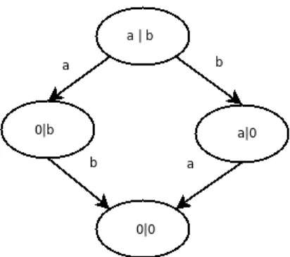
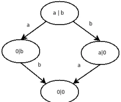
As an example lets take the process defined asa.0|b.0, which we will abbreviate by omit-ting the empty processes at the end to a|b. This process is capable of evolving through two possible transitions by using any of the two first rules in figure 2.2 which are possible because the subprocessesa.0andb.0are capable of performing a transition using the rule for prefix, by performing an action,aorbrespectively, and evolving to the empty process. Figure 2.3 depicts the LTS built by fully analyzing process a|b. The first, top-most, tier shows the originating process with the two transitions we just described; in every state in the second tier one of the subprocesses of the composition is not capable of performing any action, and thus each state has only one edge leading from it to the final state of the system, where none of the subprocesses is capable of performing any action, and as a consequence neither is their composition.
2.2.2 π-calculus
Figure 2.3 LTS for a simple CCS process
π F x(y) receive y along channel x
x<y> send y along channel x
τ unobservable action
P,Q F Pπi.Pi (summation) | P|Q (composition) | (νc)P (restriction)
| !P (replication)
Figure 2.4 Theπ-calculus
by allowing fresh names to be generated and for those names to be passed along in communi-cations where they can be used as channel names. Figure 2.4 shows the syntax of the resulting calculus.
What this calculus adds in terms of expressiveness is the fact that names can not only be generated by the (restriction) construct, but they can also be passed along and received by other processes. The act of receiving a name through a channel binds the receiving variable to the sent name which can also be used as a channel.
Figure 2.5 shows an example of a system which makes use of the mobility of channels. There are three types of participants in the system: A, which sends and receives a message through a single channel; Talk, which receives and sends a message through a channel plus is capable of receiving another channel which will start being used in the receive-send cycle; and C, which decides whether or not it is time for Talk to switch channels. The mobility in this example is present in how Talk can change the connection it is using by “order” of process C. This example illustrates, in a very simple setting, how process names can be passed along with messages in theπ-calculus. These language mechanics are used in [22] to model the handover protocol between mobile phone stations and the mobile devices while they are moving.
C(x1,x2) , τ.C(x1,x2)
+switch<x1>.C(x1,x2)
+switch<x2>.C(x1,x2) T alk(c,m) , c(m).c<m>.T alk(c,m)
+switch(c1).T alk(c1,m) A(x,m) , x<m>.x(m).A(x,m) S ys , (νx1,x2,m)
(T alk(x1,m)|C(x1,x2)|A(x1,m)|A(x2,m))
Figure 2.5 A simple example of mobility
it happens that the added power the possibility of exchanging channel names brings to the language allows it to model theλ-calculus thus making it Turing Complete, which is interesting to note.
2.2.3 Bisimulation
One of the verifying techniques mentioned before is the use of a relatively simple specification process and comparing it to a process modeling the actual implementation we want to verify to check if the behavior is the expected one. Equivalences like structural congruence are not expressive enough to compare processes for this purpose as it is possible for a non-congruent processes to behave in the same manner. One such example are the processesa|banda.b+b.a which are not structurally congruent but exhibit the same behavior: can either reada and then b or vice-versa. In order to compare these processes we need to define a broader sense of equivalence where we take into account the behavior of processes instead of just their syntactic similarities. The behavioral equivalence between CCS processes is elegantly captured by the notion of bisimulation where processes are equivalent if and only if they can mutually simulate each other.
Formally, bisimulation is a relation between labelled transition systems which deems sys-tems equivalent if and only if they are only able to perform equivalent transitions. This means that two processes, or sub-processes, related by a bisimulation can be interchangeably switched without any difference in the overall behavior of the system. Two processes P and Qare in a bisimulation if and only if the following two conditions hold:
1. IfP−→α P′, then there existsQ′such thatQ−→α Q′andQ′is bisimilar toP′.
2. IfQ−→α Q′, then there existsP′such thatP−→α P′andP′is bisimilar toQ′.
In , in.m.In Out , m.out.Out Sys , (In|Out)\ {m}
Spec , in.out.S pec
Figure 2.6 Example of weak bisimulation
have a similar structure to the one depicted in figure 2.3. The bisimulation relating the two processes makes a one to one correspondence between the identical nodes of the LTS.
The bisimulation relation defined above forces processes to have the exact same behavior in order for it to be applicable, which may not be entirely desirable as internal behavior must also match. This makes specifications to be used with this kind of equivalence relation be more complicated than needed whereas simpler specifications should be able to describe the intended behavior.
To get simpler specifications we may abstract from the internal details of the systems and compare them using only their observable behavior, from where we excludeτtransitions. For an observer a process which doesτ.τ.a.τbehaves in exactly the same manner as a process which only performs a. For that observer there is no discernible difference in the behavior of the two
processes (regarding the mentioned transition), making them equivalent to said observer. The notion of bisimilarity mentioned above does not consider two processes with these transitions equivalent but we may want to consider them as if they were.
It is possible to define a different notion of bisimilarity where processes are equivalent if
and only if they are capable of making the sameobservabletransitions to equivalent states. The bisimilarity characterization for this notion of equivalence can be obtained from the definition of bismilarity given above by exchanging the transitions with a different notion of transition
where non-observable actions are not taken into consideration. A transitionP=α⇒P′is possible whenever a process P can evolve to a processP′ by performing a possibly empty series ofτ transitions, followed by a transition byαand another possibly empty series ofτtransitions. We defineweakbisimilarity by replacing the−→α transitions with=⇒α transitions. With the notion
2.3
Logics
When reasoning about a concurrent system described in some calculus like CCS or the π -calculus, one cannot derive all interesting properties from just structural properties or behavioral equivalence. In order to reason about higher level properties of systems it is often convenient to express them in specially tailored logics and devise an algorithm for checking if a process satisfies a formula in that logic. These algorithms are called model checking algorithms and we will discuss them in section 2.4.
Special logics have been formulated to express temporal and behavioral properties of sys-tems. Temporal logics, like LTL[25] and CTL[7], allow us to reason about the timing of the sat-isfaction of properties. Some examples of temporal logic predicates include assessing whether a property will hold eventually in the lifetime of the system, or if it always holds. Behavioral log-ics, like Hennessy-Milner’s and the µ-calculus, allow us to reason about behavioral properties of systems. One example of a behavioral predicate is the possibility for performing an action to reach a state satisfying a given property, which can be used to assess whether a process is in a deadlock state, for instance.
On the remainder of this section we will describe two behavioral logics, Hennessy-Milner’s and theµ-calculus. We focus on the behavioral kind of logics because they are best suited for describing the behavior of concurrent systems, which makes them of particular interest for the purposes of this thesis.
2.3.1 Hennesy-Milner Logic
Matthew Hennessy and Robin Milner proposed a logic for reasoning about labelled transition systems in [15]. The logic they proposed consists of the propositions described in figure 2.7 ac-companied by the satisfaction rules in figure 2.8. This logic, besides the usual logical operators, adds the modal behavioral operators which allow reasoning about a process’ transitions. (dia-mond) states that a process must evolve to a state satisfyingΦby doing a transition with label
α, and (box) states that all transitions by labelαmust reach a state satisfyingΦ. One interesting
aspect of these operators is that even though (box) can be defined in terms of (diamond), we cannot define (diamond) in terms of (box): [α]Φ is equivalent to¬<α>¬Φ, which intuitively
states that it is not possible to do a transition usingαwhich does not lead to a state satisfying
Φ; but it is not possible to write a property equivalent to <α>Φusing only the other operators
in the logic. Even though the logic could be smaller, we keep the (box) operator because its expressiveness is very useful in defining properties.
The example process we used in section 2.2.1 satisfies the following property which states that it can perform either ana transition or abtransition: <a>⊤∧<b>⊤. Another property we
can define is [a](<b>⊤∧ [a]⊥) which states that if it is possible to perform a transition with
labela, after doing it it is possible to do a transition by readingbbut not by readinga.
Φ,Ψ F ⊤ (true)
| ⊥ (false)
| Φ∨Ψ (or)
| Φ∧Ψ (and) | ¬Φ (negation) | <α>Φ (diamond) | [α]Φ (box)
Figure 2.7 Hennessy-Milner logic
E⊤
E2⊥
EΦ∧Ψ iif EΦand EΨ
EΦ∨Ψ iif EΦor EΨ
E¬Φ iif E2Φ
E<α>Φ iif ∃F∈ {E′:E−→α E′} FΦ
E[α]Φ iif ∀F∈ {E′:E−→α E′} FΦ
Figure 2.8 Hennessy-Milner Logic’s semantics
capable of distinguishing two strongly bisimilar CCS processes.
2.3.2 µ-calculus
The Hennessy-Milner Logic (HML) which we described in the previous section is only capable of reasoning about finitely many transitions, as all have to be explicit. This restriction makes it unsuitable to reason about eventual (something will happen in some future state) or permanent (something always happens) properties. To address this lack of expressiveness an extension of HML, called theµ-calculus, was devised by de Bakker in [1].
Theµ-calculus extends HML by adding fixed point operators which allow recursive property definitions. The added operators are µ.X(Φ) andν.X(Φ) for minimal and maximal fixed point
on formula X, respectively.
Using these new operators one can define properties like “it is always possible to perform a transition by readinga”,ν.X(<a>⊤∧[−]X), or “sometime in the future, this process will be able
2.4
Model Checking
Model checking, introduced by Clarke, Emerson and Allen in [6], consists of checking whether a model, formulated in some algebraic language, satisfies a given logical formula and origi-nally appeared as a technique for verifying if digital circuits corresponded to their specification. Model checking has the restriction of only being applicable to finite state systems which con-fers it the property of being able to be performed automatically. A bonus of being applicable only to finite systems is that we gain the certainty that, given enough resources, the recursive model checking algorithm will eventually terminate. However, when used in the context of verifying large concurrent systems model checking suffers from the problem of state
explo-sion where there may be simply so many states to check, due to their exponential growth from non-determinism, that in practice the algorithm will take too much time to execute or not have enough resources to deal with the problem at hand.
In order to cope with the state explosion problem and be able to verify larger systems there are several techniques available to both the implementers of model checking algorithms and to the people specifying systems to be model checked. Some of these techniques are used to reduce the resource usage of the algorithm, by using a more succinct representation for the system states (ordered binary decision diagrams as in [3], for example), or the running time of the algorithm, by checking only a possible subset of interleaving actions built from partial orderings[14] of independent actions. Apart from the algorithmic improvements which can be done, system specifiers can also abstract some parts of the system to smaller subsystems with identical properties in order to minimize the number of states in the whole system. There are many other aspects of the system, like symmetry for one, which can be exploited to allow this technique to be employed on even larger systems.
Using model checking on a system has three stages: Modeling the system by converting it to a formalism accepted by the model checking tool; Specifying, using an appropriate logic, which properties are desired that the system verifies; and the actual Verification which is, ideally, done automatically by a tool.
2.5
Techniques for bisimulation checking
In order to compare two processes to check if there is a bisimulation relating them, i.e. they are bisimilar, it is possible to create the full transition graph and attempt to build the bisimulation relation by using its definition directly. This however is very time consuming and impractical for most but the smallest processes. To be able to cope with the number of states a reasonably larger system has, it is necessary to use better techniques for bisimulation checking.
There are a couple ways which have proven to be successful in dealing with creating a bisimulation relation: partition refinement algorithms and “on the fly” verification techniques are the most prominent.
processes can be seen as a partition refinement problem. A simplistic view of this approach is that we can start with all the states in a single partition, considering them all equivalent, and then iteratively refine the partitions based on which transitions are possible in a state until a fixed point is met. Once no more refinements are possible, the bisimilarity test is simply a matter of checking whether the starting points of the processes being compared ended up in the same partition, i.e. the same class relating to the notion of equivalence used in the partitioning. There are several optimizations which can be employed in order to reduce the running time of the algorithm, being that currently the most efficient are the ones due to Paige and Tarjan in
[23].
The above mentioned technique deals with the problem of exhaustively searching the state space to build a bisimulation relation in an efficient manner. Another way to allow verification
of larger systems is by reducing the space complexity of the algorithm, which Fernandez and Mounier showed to be possible in [11]. The algorithm they propose does a Depth-First Search of the space state instead of expanding it fully, making it require a lesser amount of memory resources.
This technique was employed in the Aldébaran tool in order to improve the efficiency of its
bisimilarity checker, but the former technique is by far the most widely spread being used in the majority of tools which support equivalence checking of some sort.
2.6
Tools which support bisimulation checking
Bisimilarity checking is implemented in a reasonably large number of tools. Most of these tools support the specification of processes based on some process calculus and incorporate bisimilarity checking using one of the above discussed algorithms. In this section we discuss some well known tools.
Victor and Moller’s Mobility Workbench[29] (MWB) is much like the Concurrency Work-bench (CWB) of Cleaveland, Parrow and Steffen[9] in terms of functionality, but they differ
in the specification language used. They work on different base languages, CWB uses CCS
while MWB is based on the π-calculus, but both provide a fairly wide range of equivalence relations to compare processes with. CWB provides strong and weak bisimilarity while MWB can be used to compare processes with strong, weak, and open bisimilarity. They also differ in
what algorithm is used when checking for equivalence between processes. CWB uses partition refinement but due to the dynamic nature of the π-calculus, the authors of MWB cannot use partition refinement algorithms for bisimilarity checking and use the “on-the-fly” techniques to implement the equivalence test.
The SIGREF tool[31] employs Binary Decision Diagrams (BDDs) to shorten the repre-sentation of the transition graphs used in the partition refinement algorithm used to check for branching bisimilarity between CCS-like processes.
standard based on CCS and CSP. This tool allows for strong and weak bisimilarity comparison between processes and implements almost every mentioned technique. The tool uses a partition refinement algorithm with BDDs but can also use “on-the-fly” techniques when appropriate.
2.7
Spatial Logic Model Checker
The Spatial Logic Model Checker (SLMC) developed by Hugo Vieira, Luís Caires and Ruben Viegas[30] is a model checking tool written in OCAML which incorporates a process defini-tion language based upon the π-calculus, and a logical specification language which includes behavioral and spatial properties[4].
In this chapter we introduce the possibility to use a logical formula to assert whether or not a process is bisimilar to another and provide some algorithms to build such formulae based on CCS processes. We provide some examples of application of this technique and discuss its limitations and how we can overcome them.
3.1
Building Characteristic Formulae for CCS Processes
The equivalence relation induced by a given logic over two programs is usually given in the terms of whether or not it is possible to devise a formula in the logic which can differentiate the
two processes. In simpler terms, two processes are equivalent in regard to a certain logic if for any formula one of the processes satisfies, the other also satisfies the same formula.
Using this result directly would involve going though all possible formulae and checking if the two processes provided the same result for each formula (although search space can be reduced, it would always be rather big). Another, more suitable, approach to using this result to verify process equivalence is by attempting to build a distinguishing formula. Such a formula would be satisfied by one process and not by the other therefore the logic would be capable of revealing that the processes are not equivalent. How to build a distinguishing formula is well known, and is used in several tools, like the Concurrency Workbench, to provide better feedback on the user in understanding why a process is not equivalent to another.
Building a formula capable of distinguishing two processes is interesting but requires that both processes to be compared be known. It would be even more interesting to be able to build a formula, named a characteristic formula, from one of the processes which could be used to assert whether or not any other process is equivalent to the one which originated it. This formula would attest to the complete behavior of the process up to bisimulation given certain conditions on the compared process were satisfied.
The first step towards building a characteristic formula from a CCS process was given by Graf and Sifakis in [26] where they describe a function between a process and a formula which provides characterization up to bisimilarity. The logic used is very similar to Henessy-Milner’s while the process calculus is basically CCS without the parallel composition operator or re-cursion. The expressive power of the model is basically the same as CCS since it is always possible to rewrite a process with parallelism into a process with only choice by enumerating all possible interleavings of the parallel compositions’ transitions. Another way to interpret the process calculus they used in this paper is by treating it as a calculus which describes an LTS, since it describes the different actions a process can do at any given point.
In [27] Steffen extends Graf and Sifakis’ approach to also be able to deal with recursively
defined processes, as long as the process is finite state. Steffen’s way to build characteristic
formulae is based on the LTS of a process and uses a fixed point operator from the modal µ-calculus to deal with recursion.
In the next two sections we will describe how to build characteristic formulae based on a Labelled Transition System given by a quadruple (S,Act,T,s) where:
• S is a (finite) set of states. • Actis a (finite) set of actions.
• T is a functionS×Act×S relating how a state can evolve to another state by performing an action.
• sis the initial state.
On each section we will also show how a characteristic formula looks like for a few sim-plistic examples.
3.1.1 Finite Processes
We can describe the generation of the characteristic formula for an LTS through a functionT r applied to the initial state of the LTS which is defined for any state in the LTS as follows:
^
a∈B
<a>T r(s′) ∧ ^
a∈Act
[a] _
s′∈C(a)
T r(s′) (3.1)
Where
• Bis{a: a ∈ Act ∧ ∃ s′ : (s,a,s′) ∈ T} • C(x) is{s: s ∈ S ∧ ∃(s,x,s′) ∈ T}
Following the usual convention thatV∅istrueandW∅is f alse, this method of building a
formula equates to having for each state a formula which is a logical conjunction of:
1. <α>sfor each transitionαleading to the state satisfying s.
2. [α](s1∨s2∨...∨sn) for all states (s1 tosn) lead to by labelα, for everyαwith a transition in that state.
3. [α]⊥for all transitionsαnot possible in that state.
Figure 3.1 The LTS for processa|b.
s3 = [a]false and [b]false
s1 = <a>s3 and [a]s3 and [b]false s2 = <b>s3 and [b]s3 and [a]false
s0 = <a>s2 and <b>s1 and [a]s2 and [b]s1
Figure 3.2 Formulae for characterizinga|b.
3.1.1.1 Examples
To illustrate the construction of a characteristic formula for a finite process we will see how it is built for processa | b, and then reason that processa.b + b.a, which is well known to be bisimilar to the first process, satisfies the introduced formula. We will also exemplify how can non-bisimilar processes be identified as such by the built formula.
The process a | b has the LTS depicted in figure 3.1, where from the initial state it is possible to performaorb, on the final state no actions are possible and there is a state for each transition in the initial state where it is possible to do a transition to the final state using the action which was not the one leading to that state.
Figure 3.2 shows the characteristic formulae for the above mentioned process. Property s3 describes the behavior of the bottom state in the LTS of figure 3.1, where no action is possible. The formulaes1ands2describe the intermediate states whereborawere performed, respectively, from the initial state. In these states it is possible to perform a, respectively b, leading to a state satisfyings3, andb, respectivelya, cannot be performed in states satisfying these formulae. The initial state for the process yields formulas0from figure 3.2. This formula states what transitions can be done, namely one using label a to a state satisfyings2and one using labelbto a state satisfyings1. The formula also asserts that all transitions by labelamust lead to a state satisfyings2and similarly tobands1.
a.b + b.a + a.asatisfy or not the characteristic formula we came up with fora|b.
Processa.b + b.ais known to be bisimilar toa|b, so it should satisfy the formula. On its initial state it can performaorb. If it performsa it will arrive in a state where it can dob and become inactive, which satisfies formulas2. If it performsa, it transforms into a process which satisfiess1as it can, and can only, performbafter which it becomes inactive.
Process a.b should not satisfy the characteristic formula for a|b, and it indeed fails to satisfys0from the fact that it cannot performbon its initial state.
Processa.b + b.a + a.ashould not satisfy s0. It perfectly satisfies<a>s2, <b>s1 and [b]s1, but fails to satisfy[a]s2 as there is a transition bya to a state which does not satisfy s2, but instead satisfiess1.
The three examples in the previous discussion try to illustrate how the characteristic for-mulae devised by Graf and Sifakis detect deviant behavior from the process which originated the formula. We exemplified what happens when the process does behave correctly, how the formula detects some transition is missing and how it detects that some transition is there when it should not be.
This method for building characteristic formulae is the basis for the method we explain in the next section which extends it in order to add support to infinite behavior as long as the process has a finite number of states.
3.1.2 Finite State Processes
Building a characteristic formula for finite state processes which may have recursive, and there-fore infinite, behavior requires that the logic in which we express the formula also allows the definition of recursive formulae. For this purpose we use the modal µ-calculus to make use of its fixed point operators to construct the desired formula.
Dealing with infinite behavior using the approach described in the previous chapter would result in formulas with infinite size due to the fact that recurrent states would always be revisited. In order to cope with this issue we need to be able to represent infinite behavior in a finite fashion and that is where the novel operators in theµ-calculus come into play, by allowing some form of recursion in logical formulae.
In [27] Steffen was the first to provide an algorithm which allows translating a CCS-like
pro-cess into a characteristic formula in theµ-calculus. Steffen’s approach is based on the
“rewrit-ing” of the LTS to turn it into a regular tree so that it is possible to do the depth-first application of an algorithm which introduces fixed-point calls when they are needed. His algorithm has two steps, one initialization step and one depth-first association between each node and a formula for that node:
1. Initialization: Assign a fresh variable to every node. 2. Formula: In depth-first order do, for every node:
SemSpec = p.Sem1
Sem1 = p.Sem0 + v.SemSpec Sem0 = v.Sem1
Sem = p.v.Sem SemGood = Sem | Sem
SemBad = p.v.SemBad + p.p.v.v.SemBad
Figure 3.3 Semaphores
• replace the currently assigned formula with the formula built in the previous step with a fixed point “around” it using the node’s current formula as the fixed-point variable.
Instead of analysing the LTS and building the equivalent regular tree, it is possible to achieve the same result by depth-first searching the LTS and maintaining a list of nodes in the path to the current node. Whenever a transition leads to a node in the path, it is a back-arc and a variable should be used instead of further building the formula.
3.1.2.1 Examples
We will now provide two examples of how to use this method to build characteristic formulae. In the first example we will try to distinguish a good and a bad implementation of a two unit semaphore by providing a specification of the behavior of the semaphore, a good implementa-tion by composing two one unit semaphores in parallel and a bad choice based implementaimplementa-tion. On our second example we will show why the transformation of the LTS into a regular tree is necessary in order for the algorithm provided by Steffen to work.
On our first example we use the processes defined in figure 3.3 where we can see the defini-tion of four processes: a specificadefini-tion for a two-unit semaphore (SemSpec), the implementadefini-tion of a one unit semaphore (Sem), the implementation of a two-unit semaphore by parallel com-position of two one-unit semaphores (SemGood), and the failed attempt at the definition of a two-unit semaphore using only choice (SemBad). We will build the characteristic formula for SemSpec and check whether GoodSem and BadSem satisfy it so as to identify which of them correctly implements a two-unit semaphore.
Figure 3.4 LTS forSemSpec.
semspec = maxfix SemSpec.(
<p>sem1 and [p]sem1 and [v]false)
sem1 = maxfix Sem1.(
<p>sem0 and <v>SemSpec and [p]sem0 and [v]SemSpec) sem0 = maxfix Sem0.(
<v>Sem1 and
[v]Sem1 and [p]false)
Figure 3.5 Characteristic formula forSemSpec.
Figure 3.4 depicts the LTS for SemSpec, based on which we will build the characteristic formula for that process. The LTS is already a regular tree, which means no transformation is necessary in order to correctly apply Steffen’s algorithm. Using Steffen’s algorithm we come
up with the formula depicted in figure 3.5, where uncapitalized variables are to be taken as full text substitutions by the appropriate formula while capitalized variables are fixed point “calls” and are to be taken as is.
Figure 3.6 LTS for processS.
p, and is able to performvby reacting with either of the processes in the parallel composition, where it becomes v.Sem|Sem or Sem|v.Sem, both of which are structurally congruent and, by the fixed point hypothesis, satisfy Sem1. From this we can conclude that GoodSem satis-fiessemspecand is therefore correctly identified as bisimilar toSemSpecby the characteristic formula.
On the other hand,BadSemmight also seem to have a behavior compliant withSemSpec, as it can either performp and thenv, orptwice and thenv twice before returning to the starting state. However this process has the problem of making a premature “decision” about what case it is expecting. After performing the first reaction by actionpthis process transforms into either v.BadSem orp.v.v.BadSemwhich means in one case it can only performv, and in the other it can only perform p, negating the possibility for the environment to choose which action to perform. This misbehavior is caught on by the characteristic formula by forcing all states after performing a pfrom the original one to satisfysem1. Neither of the possible continuations for BadSemis capable of satisfyingsem1because it will either not allowporv.
We will use the recursive processS = a.a.S + a.a.a.Sto illustrate the need to turn the LTS into an equivalent regular tree so that Steffen’s algorithm can be used. This process’ LTS
has three states as depicted in the left side of figure 3.6. If we were to apply Steffen’s algorithm
s0 = maxfix S0.(
<a>s1 and <a>s2 and [a](s1 or s2)) s1 = maxfix S1.(
<a>S2 and [a]S2) s2 = maxfix S2.(
<a>S0 and [a]S0)
maxfix S0.(
<a>maxfix S1.(<a>S2 ... ) ... )
Figure 3.7 Erroneous formula forS.
3.2
Challenges
The main issue with the approach described in this chapter for the generation of characteristic formulae is the amount of space which the formula itself requires. We shall illustrate this matter using the semaphore example in figure 3.5.
Formulasem0appears twice in formulasem1which in turn also has two copies in formula semspec, which means formulasem0ends up repeated four times in the final formula used to characterize the behavior of theSemSpecprocess. More complicated processes will suffer the
same problem and exhibit an even greater blowup in size if there is the possibility of reaching a state by several possible paths in the LTS, as that whole state’s characteristic formula needs to be repeated in all the possible paths in the formula.
Even if we can somehow eliminate the space requirement for the formula, the underlying reason for the issue still exists and will manifest itself when we attempt to analyze the new process. The deeper problem is that we need to traverse all possible paths and assert that all of them are in conformity with the behavior of the system which originated the formula, even if we get to that a similar state from a different path. There is a lot of redundancy in these formulae
which needs to be dealt with in order for this approach to be viable.
In our implementation we overcome the space challenge by using a characteristic equation system instead of a single formula. The use of this equation system means that the formula for each state is only defined once and an abbreviation of it is used in all the places where it would appear. This eliminates redundancy in the formula, reducing its size.
The work performed for this thesis was based on SLMC, an already existing tool which sup-ports Spatial Model Checking on a π-calculus like language using a logic which extends the µ-calculus with spatial properties. In this chapter we describe the tool as it was and how it has become as a result of this work. We also describe the inner workings of the new functionalities and provide an in-depth discussion of the choices made.
4.1
The Spatial Logic Model Checker
The Spatial Logic Model Checker is a tool which allows the automatic verification of behavioral and spatial properties of processes described in a process language similar to the π-calculus. Besides the operators from the µ-calculus SLMC introduces operators capable of reasoning about the structure of processes. In the following subsections we will present the language for processes and the language used to express properties of those processes. We will also provide some insight on the meaning of the formulae.
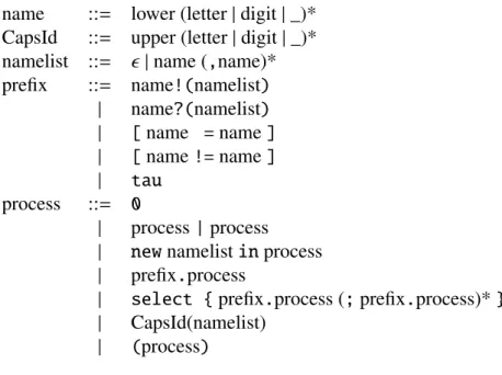
4.1.1 Syntax of Processes
Processes in SLMC are defined using the language shown on figure 4.1. This language is basi-cally theπ-calculus where sending a message with arity two in channelais writtena!(m,n), and receiving one is writtena?(x,y). We also have the choice operator which is here written using theselectconstruct instead of a+operator. As the language accepted by SLMC is based on the polyadicπ-calculus, when sending or receiving messages in channels, they can exchange any number of names. In this language it is also possible to represent the internal silent (un-observable) action, and compare names by their equality (or inequality). As we will see, it is possible to define processes based on others, so there is a construct which allows using another process’ definition to aid in the construction of a given process. It is also possible, using the newconstruct, to declare fresh names private to the enclosed process.
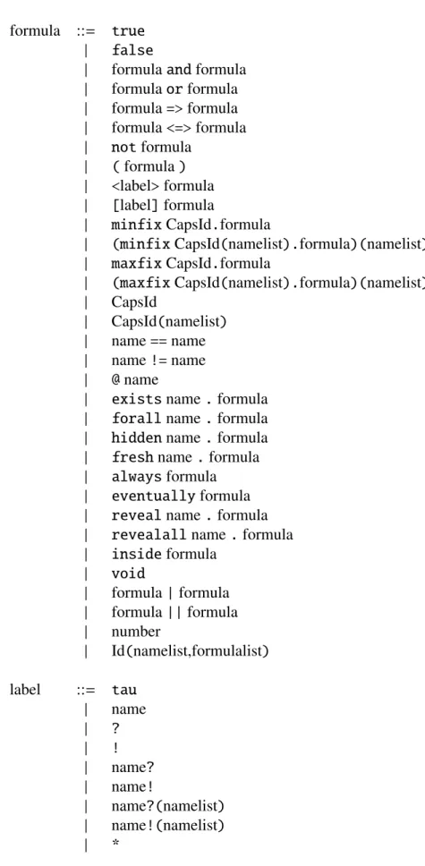
4.1.2 Syntax of Formulae
Formulae in the SLMC have the typical logical connectives and constants, to which they add the Hennessy-Milner modalities for possibility and necessity of an action. We can also define recursiveness in formulae by using the maximum and minimum fixed point operators which are also able to be parametrized. In addition to this there are also a few quantifiers over names: the existence quantifier,exists; the universal quantifierforall; and quantifiers for fresh and hidden names, respectivelyfreshandhidden. The temporal modalityalwaysexpresses that a formula is satisfied in all configurations of a system with regard to its internal evolution. Theeventuallymodality states that a property will be true after some unspecified number of
name ::= lower (letter|digit|_)*
CapsId ::= upper (letter|digit|_)*
namelist ::= ǫ |name (,name)*
prefix ::= name!(namelist)
| name?(namelist)
| [name =name]
| [name!=name]
| tau
process ::= 0
| process|process
| newnamelistinprocess
| prefix.process
| select {prefix.process (;prefix.process)*}
| CapsId(namelist) | (process)
Figure 4.1 Syntax of SLMC processes.
internal steps.
It is important to be aware of what the various possible labels for the behavioral modalities of the logic mean:
• tauor an empty label, denote an internal computation step.
• namedenotes any action, either input or output, with subjectname. • ?denotes any input action.
• !denotes any output action.
• name?denotes any input action with subjectname. • name!denotes any output action with subjectname. • name?(namelist)denotes a particular input action. • name!(namelist)denotes a particular output action.
Finally, when defining a property there is also the possibility of using another, already de-fined property, by using the property’s name, which can be parametrized in both names and other formulae.
The logic presented here induces a form of equivalence which is stronger than bisimilarity as it is capable of distinguishing processes based on their structure, instead of just on their be-havior like what happens with theµ-calculus. An example of this property is that the processes a.b+b.a and a|b, can be distinguished by the formula not void | not void while they cannot be distinguished by any formula in theµ-calculus. The complete characterization of the equivalence induced by the logic the SLMC tool uses is further described in [5]. As the main interest in this work is in characterizing bisimilarity we will not be making use of the spatial operators present in the logic.
4.1.3 Top Level Commands
The SLMC tool is used by issuing one or more of several top level commands. The basic func-tionality provided by these commands includes the definition of both processes and properties and the possibility to check if a process satisfies a property.
4.1.3.1 Defining Processes
To define a process in SLMC we use thedefproccommand. Thedefproccommand is issued in the following manner:
defproc ID[(n1,...)] = <process> (and ID[(n1,...)] = <process>)*;
We can create a process by specifying an identifier for it, a possibly empty list of parameters and its definition using the process language described previously. Processes can be recursive and, more interestingly, mutually recursive as we can define several processes at once, using the and connective. The process identifiers need to start with a capital letter. We now define the simple processa|bin SLMC:
defproc Simple = a?() | b?() ;
formula ::= true
| false
| formulaandformula
| formulaorformula
| formula=>formula
| formula<=>formula
| notformula
| (formula)
| <label>formula | [label]formula
| minfixCapsId.formula
| (minfixCapsId(namelist).formula)(namelist)
| maxfixCapsId.formula
| (maxfixCapsId(namelist).formula)(namelist)
| CapsId
| CapsId(namelist)
| name==name
| name!=name
| @name
| existsname.formula
| forallname.formula
| hiddenname.formula
| freshname.formula
| alwaysformula
| eventuallyformula
| revealname.formula
| revealallname.formula
| insideformula
| void
| formula|formula
| formula||formula
| number
| Id(namelist,formulalist)
label ::= tau
| name
| ?
| !
| name?
| name!
| name?(namelist) | name!(namelist)
| *
defproc SemSpec(p,v) = p?().Sem1(p,v)
and Sem1(p,v) = select {
p?().Sem0(p,v) ; v?().SemSpec(p,v) }
and Sem0(p,v) = v?().Sem1(p,v) ;
4.1.3.2 Defining Properties
In SLMC it is possible to define a named property through the use of thedefpropcommand. This command is very similar to the defproccommand except that property identifiers need to start with a lowercase letter and we cannot define mutually recursive properties. In order to define recursive properties we have to rely on the logic’s fixed point operators instead of being able to use a formula’s own identifier to recursively refer to it. The concrete syntax for defining a formula is given bellow, where a property can be parametrized in a set of names and/or in a
set of other properties.
defprop id[(n1,...,P1,...)] = <formula>;
An example of the definition of a property in SLMC could be property semstart which states that it is possible to performgetbut notput. This property can be defined in SLMC as
defprop semstart =
<get>true and [put]false ;
However, as our two unit semaphore is parametrized on the names of the channels to be used for communication, we might want to also parametrize our property on the names to be used. In addition we might want that the behavior after the first get also be given as a parameter in order to be able to use the same definition to check whether the first state is correct or to be able to check more deeply the process’ behavior. One possible definition for the newsemstart property could be the following
defprop semstart(p,v,C) = <p>C and [v]false ;
4.1.3.3 Checking Properties of Processes
Verifying if a process satisfies a certain property is done via thecheckcommand, which is used in the following manner:
check <process id> [(n1,...)] |= <formula>;
In this command one check whether an already defined process satisfies a formula. Unlike the process which must have already been defined via thedefproccommand, the formula can be definedin-loco. We can check that theSimple process is capable of performing both ana and abtransitions by issuing the following command:
check Simple |= <a>true and <b>true;
We can also check properties which were already defined, for instance thatSemSpecsatisfies semstart(with the proper parameters).
check SemSpec(get,put) |= semstart(get,put,true);
As was mentioned earlier, we can also use the semstart property to use more complex properties in its third parameter. For example, we can check that the process following aget can perform anotherget, and also aput.
check SemSpec(get,put) |=
semstart(get,put,<get>true and <put>true);
4.1.3.4 Additional Commands
To facilitate the development and verification of more complex systems or examples, it is pos-sible in SLMC to issue a command which reads a file containing other commands. The load command takes a file name enclosed in double quotes and reads commands from it. The file-name can be relative to the current working directory or absolute in the file system, as expected. To allow the user to inspect and change the current working directory, SLMC provides the top level commandspdandcdto respectively perform those actions.
showing a count of the number of times some property was checked against a process during the checking of a bigger property; the integer parameter max_threads controls how many transitions there must be in a process for it to be considered unmanageable by the system. The max_threadsparameter is used to provide a cut-offpoint when processes seem to belong to
the class of processes for which the model checking algorithm does not terminate.
4.2
Extensions to the Tool
We have implemented a few extensions for the SLMC tool to permit its usage as a tool for checking bisimilarity between processes. The implemented extensions include a way to di-rectly check the bisimilarity of two processes and an operator in the logic which allows the construction of a characteristic formula. As some sort of side effects from the development of
these functionalities there was also the introduction of a new modality into the logic and the implementation of a feature which allows observing a process’ behavior.
In the remainder of this section we will describe the interface to the introduced functionali-ties, while on the next section we discuss their implementation details.
4.2.1 Process Stepping
We have implemented a feature which allows a user to interact with a process in a step-by-step manner. This feature allows the user to select one of the possible actions a process can perform and evolves the process according to the user’s selection. It is capable of detecting when the process cannot perform any action and when a process is at a repeated state.
We can access this functionality by issuing thestepcommand as follows:
step P[(n1,...)];
> step SemSpec(get,put) ; Stepping SemSpec(get,put) free names: put, get
restricted names:
Please select a transition to follow, type ’q’ to quit: 1: <get?()>
goto> 1
restricted names:
Please select a transition to follow, type ’q’ to quit: 1: <put?()>
2: <get?()> goto> 2
restricted names:
Please select a transition to follow, type ’q’ to quit: 1: <put?()>
goto> 1
YOU HAVE ALREADY BEEN TO THIS STATE restricted names:
Please select a transition to follow, type ’q’ to quit: 1: <put?()>
2: <get?()> goto> 1
YOU HAVE ALREADY BEEN TO THIS STATE restricted names:
Please select a transition to follow, type ’q’ to quit: 1: <get?()>
goto> q >