Numerical solution to generalized Burgers'-Fisher equation using Exp-function method hybridized with heuristic computation.

(1)

Numerical Solution to Generalized

Burgers'-Fisher Equation Using Exp-Function Method

Hybridized with Heuristic Computation

Suheel Abdullah Malik1*, Ijaz Mansoor Qureshi2, Muhammad Amir1, Aqdas Naveed Malik1, Ihsanul Haq1

1Department of Electronic Engineering, Faculty of Engineering and Technology, International Islamic University, Islamabad, Pakistan,2Department of Electrical Engineering, Air University, Islamabad, Pakistan

*suheel.abdullah@iiu.edu.pk

Abstract

In this paper, a new heuristic scheme for the approximate solution of the generalized Burgers'-Fisher equation is proposed. The scheme is based on the hybridization of Exp-function method with nature inspired algorithm. The given nonlinear partial differential equa-tion (NPDE) through substituequa-tion is converted into a nonlinear ordinary differential equaequa-tion (NODE). The travelling wave solution is approximated by the Exp-function method with un-known parameters. The unun-known parameters are estimated by transforming the NODE into an equivalent global error minimization problem by using a fitness function. The popular ge-netic algorithm (GA) is used to solve the minimization problem, and to achieve the unknown parameters. The proposed scheme is successfully implemented to solve the generalized Burgers'-Fisher equation. The comparison of numerical results with the exact solutions, and the solutions obtained using some traditional methods, including adomian decomposition method (ADM), homotopy perturbation method (HPM), and optimal homotopy asymptotic method (OHAM), show that the suggested scheme is fairly accurate and viable for solving such problems.

Introduction

Most physical phenomena arising in various fields of engineering and science are modeled by nonlinear partial differential equations (NPDEs). The investigation of solutions to NPDEs has attracted much attention due to their potential applications and many numerical schemes have

been proposed, see for example [1–4]. The generalized Burgers0-Fisher equation is one of the

important NPDE which appears in various applications, such as fluid dynamics, shock wave formation, turbulence, heat conduction, traffic flow, gas dynamics, sound waves in viscous

me-dium, and some other fields of applied science [5–10].

The generalized Burgers0_{-Fisher equation is of the form [10}

–12]

utþau

d

ux uxx ¼buð1 u

d_{Þ 8}

x2 ð0_;1_Þ_;_t0 _ð₁_Þ

a11111

OPEN ACCESS

Citation:Malik SA, Qureshi IM, Amir M, Malik AN, Haq I (2015) Numerical Solution to Generalized Burgers'-Fisher Equation Using Exp-Function Method Hybridized with Heuristic Computation. PLoS ONE 10(3): e0121728. doi:10.1371/journal.pone.0121728

Academic Editor:William I. Newman, UCLA, UNITED STATES

Received:August 29, 2014

Accepted:February 15, 2015

Published:March 26, 2015

Copyright:© 2015 Malik et al. This is an open access article distributed under the terms of the Creative Commons Attribution License, which permits unrestricted use, distribution, and reproduction in any medium, provided the original author and source are credited.

Data Availability Statement:All relevant data are included within the paper.

Funding:The authors have no support or funding to report.

(2)

subject to the following initial condition

uðx;0_{Þ ¼} 1

2þ 1

2tanh

ad 2_ð_d_þ1_Þx

1_d

ð2Þ

The exact solution is given by [10–12]

uexactðx;tÞ ¼ 1

2þ 1

2tanh ad 2_ð_d_þ1_Þ x

a dþ1þ

bðdþ1_Þ a

t

1d

ð3Þ

Many researchers have investigated the analytical and numerical solutions of the

general-ized Burgers0_-Fisher_{Equation (1)}_{by using several different methods [8}

–17]. For example,

Is-mail et al. [11] used adomian decomposition method (ADM), Rashidi et al. [12] employed homotopy perturbation method (HPM), Nawaz et al. [10]applied optimal homotopy

asymp-totic method (OHAM),for obtaining approximate solutions of the generalized Burgers0_-Fisher

Equation (1). Very recently Mittal and Tripathi [8] employed modified cubic B-spline

func-tions for the numerical solution of generalized Burgers0_{-Fisherand Burgers}0_{-Huxley equations.}

Khattak [13] used collocation based radial base functions method (CBRBF) for numerical

solu-tion of the generalized Burgers0_{-Fisher equation. Javidi [14] used modified pseudospectral}

method for generalized Burgers0_{-Fisher equation.}

The Exp-function method was introduced recently by He and Wu [18] to obtain the gener-alized solitonary solutions and periodic solutions of nonlinear wave equations. The method has attracted much attention due to its simple and straightforward implementation and many

authors used it [19–24]. Among many authors, Xu and Xian [19] used Exp-function method

for obtaining the solitary wave solutions for generalized Burgers0_{-Fisher equation. Özişand}

Köroğlu[20] used Exp-function method for obtaining travelling wave solutions of the Fisher

equation. Chun[21] used Exp-function method for solving Burgers0_{-Huxley equation.}

In recent years, many authors have used heuristic computation based techniques for solving

variety of differential equations [25–35]. Very recently Malik et al. [25,26]used nature inspired

computation based approach for solving systems of nonlinear ordinary differential equations (NODEs), including biochemical reaction model [25], and boundary value problems arising in physiology [26]. Khan et al.[27] used evolutionary computation (EC) based artificial neural network (ANN)method for solving van der pol oscillator equation. Arqab et al. [28] used ge-netic algorithm (GA) based method for solving linear and nonlinear ODEs. Caetano et al. [29] used the ANN based method for solving NODEs arising in atomic and molecular physics.

The aim of this work is to obtain the approximate solution of the generalized Burgers0

-Fisher equation using a novel scheme. The scheme is based on the elegant hybrid approach of function method and evolutionary algorithm (EA). In the proposed scheme the Exp-function method is used to express the approximate wave solution with unknown parameters. The given NPDE is converted into a global error minimization problem using a fitness function with unknown parameters. Genetic algorithm (GA), one of the renowned evolutionary algo-rithms is adopted for solving the minimization problem and to achieve the unknown parameters.

To the best of our knowledge nobody as yet has tackled with the generalized Burgers0_-Fisher

equation with the scheme presented in this work. The proposed scheme is simple and straight-forward to implement and also gives the approximate solution at any value of choice in the so-lution domain. The efficiency and reliability of the proposed scheme is illustrated by solving

(3)

Materials and Methods

In this section, stochastic global search algorithm GA is introduced, the basic idea of Exp-function method is given, and description of the proposed scheme is provided.

Genetic algorithm (GA)

Genetic algorithm (GA) is one of the well-known evolutionary algorithms (EAs) that find the optimal solution of a problem from a randomly generated population of individuals called chromosome. Each individual within a population is regarded as a possible solution to the problem. The individuals within a population are evaluated using a fitness function that is spe-cific to the problem at hand. The algorithm evolves population iteratively by means of three primary operations: selection, crossover, and mutation to reach the optimal solution [36].

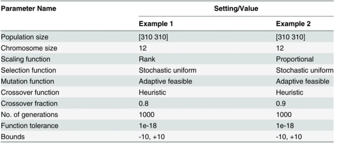
The procedural steps of GA are given in algorithm 1, while the parameters settings of the

al-gorithm used in this work are given inTable 1.

Algorithm 1.

Step 1: (Population Initialization)

A population of N individuals or chromosomes (C1,C2,. . ..,CN) each of length M is

gener-ated using random number generator. The length of each chromosome represents the number of unknown parameters.

Step 2: (Fitness Evaluation)

A problem exclusive fitness function is used to compute the fitness of each chromosome.

Step 3: (Selection and Reproduction)

The chromosomes from the current population are chosen on the basis of their fitness value which acts as parents for new generation. These parents produce children (offsprings) with a probability to their fitness through crossover operation.

Step 4: Mutation

Mutation operation introduces random alterations in the genes to maintain the genetic di-versity to find a good solution.

Step 5: (Stoppage Criteria)

The algorithm terminates if the maximum number of cycles has exceeded or a predefined fitness value is achieved. Else go to step 3.

Table 1. Parameter settings and values for GA.

Parameter Name Setting/Value

Example 1 Example 2

Population size [310 310] [310 310]

Chromosome size 12 12

Scaling function Rank Proportional

Selection function Stochastic uniform Stochastic uniform

Mutation function Adaptive feasible Adaptive feasible

Crossover function Heuristic Heuristic

Crossover fraction 0.8 0.9

No. of generations 1000 1000

Function tolerance 1e-18 1e-18

Bounds -10, +10 -10, +10

(4)

Overview of Exp-function method

Consider a nonlinear partial differential equation (NPDE) given in the following form

Nðu;u_x;u_t;u_xx;u_tt;u_xtÞ ¼0 _ð₄_Þ

Using a transformation,u(x,t) = u(η)withηdefined as follows

Z¼kxþot ð5Þ

Equation (4)is converted into a following ODE

Pðu;ku0;ou0;k2

u″; ::::Þ ¼0 _ð₆_Þ

wherekandωare unknown constants, and prime denotes derivation with respect toη.

According to Exp-function method [18], the solution of (6) is expressed in the following form

uðZÞ ¼

Xd

n¼ canexpðnZÞ

Xq

m¼ pbmexpðmZÞ

¼a cexpð cZÞ þ::::::::þadexpðdZÞ

b pexpð pZÞ þ::::::::þbqexpðqZÞ

ð7Þ

wherec,d,p, andqare unknown positive integers,anandbmare unknown constants.

The values of c and p are determined by balancing the linear term of highest order in (6)

with the highest order nonlinear term, which givesp = c[18,37]. Similarly the values of d and q

are determined by balancing the lowest order of linear and nonlinear terms in (6), which yields

q = d[18,37]. Oncec,d,p,qare determined their values are freely chosen [18]. Next the

un-known constantsanandbmare determined by substituting (7) into (6) and equating the

coeffi-cients of exp(nη) to zero, which results into a set of algebraic equations with unknown

constants. The systems of algebraic equations are solved using some software package like

Matlab, Maple or Mathematica for determining the unknown constantsanandbm,

Conse-quently the solution of NPDE (4) is obtained.

Description of the proposed scheme

We consider the NPDE given by (4) subject to the following initial condition

uðx;0_{Þ ¼}_f_ð_x_Þ _ð₈_Þ

Apply the transformation variableη= kx +ωtto (4) yields NODE given by (6). We assume

that the approximate solution of (6) is expressed in the following form in view of the Exp-function method [18].

u

__ð_Z_{Þ ¼}a cexpð cZÞ þ::::::::þadexpðdZÞ

b cexpð cZÞ þ::::::::þbdexpðdZÞ

ð9Þ

As mentioned above the values ofcanddcan be feely chosen, therefore we accordingly set

their values. The rest of the unknown parameters existing in (9) including (a-c,. . .,ad;b-c,. . .,bd;

k,ω) need to be found to obtain the approximate solution of (6). To determine the values of

these unknown parameters, the transformed NODE (6) along with the initial condition (8) is converted into an equivalent global error minimization problem by developing a trial solution

(5)

ﬁrst part represents the mean of sum of the square errors associated with the transformed NODE (6), and the second part represents the mean of sum of the square errors associated with the initial condition (8), which are given respectively as follows

"1 ¼ 1

NS

XN

i¼1

XS

j¼1

ðPðu_ðkxjþotiÞ;ku _0_ð

kxjþotiÞ;k 2

u

__″_ð_kx

jþotiÞ; :::ÞÞ 2

ð10Þ

"2 ¼ 1

S

XS

j¼1

ðu_ðxj;0Þ fðxjÞÞ 2

ð11Þ

whereNandSare the total number of steps taken in the solution domain ofxandt, andu__,_u_0_,

u__″_{are given by (9) and its derivates respectively.}

The FF which is denoted as"jis accordingly formulated as follows

"_j¼"1þ"2 ð12Þ

wherejis the generation index.

The error minimization problem given by (12) is solved using the application of

evolution-ary algorithm, such as GA, to find the optimal values of unknown parameters (a-c,. . ..ad;b-c,. . .,

bd;k,ω). Once the values of the unknown parameters are achieved, they are used in (9), which

consequently provides the approximate numerical solution of the given NPDE.

Numerical approximation of generalized Burgers

0

_{-Fisher equation}

To solve the generalized Burgers0_-Fisher_{Equation (1)}_{using the proposed scheme, we first}

apply the transformation variableη= kx +ωtwhich yield the following NODE

ou0þaud

ku0 k2

u″¼bu_ð1 ud_Þ _ð₁₃_Þ

Assume the approximate solution of (13) is given by (9) in the view of the Exp-function

method [18]. To determine the unknown parameters (a-c,. . .,ad;b-c,. . .,bd;k,ω) in (9) for

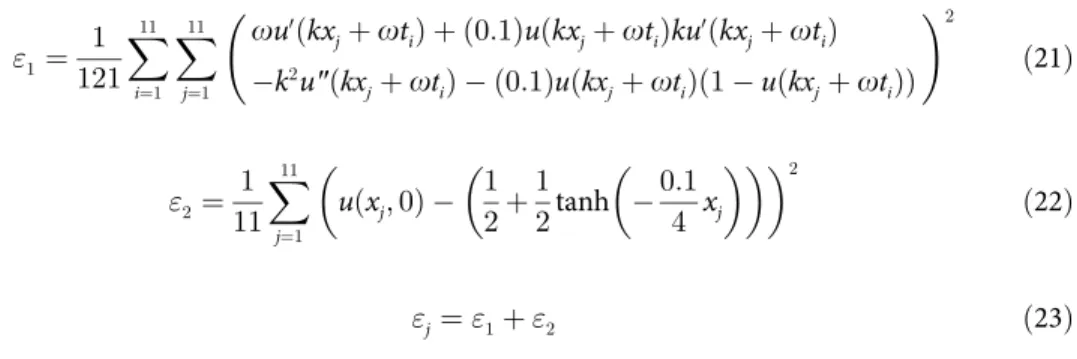
obtain-ing the approximate solution, the FF is formulated as follows (14)—(16)

"1 ¼ 1

ðNSÞ

XN

i¼1

XS

j¼1

ou0_ð_kx

jþotiÞ þau

d_ð_kx

jþotiÞku

0_ð_kx

jþotiÞ

k2

u″ðk_x

jþotiÞ buðkxjþotiÞð1 u

d_ð_kx

jþotiÞÞ

!2

ð14Þ

"2 ¼ 1

S

XS

j¼1

uðxj;0Þ 1

2þ 1

2tanh

ad 2_ð_d_þ1_Þxj

1_d!

2

ð15Þ

"_j¼"1þ"2 ð16Þ

The FF given by (16) contains unknown parameters in the form of a chromosome for GA.

The objective is to solve the global error minimization problem given byEquation (16)and to

achieve the optimal chromosome which represents the values of unknown parameters.

Conse-quently the approximate solutionu__ð_Z_Þ_{of the generalized Burgers}0_{-Fisher equation is obtained}

(6)

Convergence of the Proposed Scheme

Let the exact solution beg(η). By Exp-function method we get the solutionu(η) as follows

uðZÞ ¼a cexpð cZÞ þ::::::::þadexpðdZÞ

b cexpð cZÞ þ::::::::þbdexpðdZÞ

ð17Þ

This is a continuous function on a compact set. We apply Stone-Weierstrass theorem to

prove that for any giveng(η) on U and arbitraryε_>0, there exists a system likeu(η) as given

above such that

sup

Ujuð Þ gð Þ j< " ð18Þ

That isu(η)can be a universal approximator. For this three conditions given in

Stone-Weierstrass theorem have to be satisfied.

Let Z be a set of real continuous functions likeu(η) on a compact set U.

Condition 1: All these must be closed under addition, multiplication, and scalar multiplication.

As we can see that addition (u1(η) +u2(η)) will give same type of function. Similarly

multi-plication (u1(η) ×u2(η)) will also give same type of function, which is real, continuous and on

compact set of U. The same is true for scalar multiplication.

Condition 2: For everyη₁andη₂2U,η₁6¼η₂there exists functionu2Zsuch thatu(η₁)6¼u(η₂)

Condition 3:u(η)6¼0 for eachη2UAs we can easily judge from the function that its

numera-tor6¼0 for8ai>0,bi>0.

Thus with these three conditions satisfied, there exists forg(η) a functionu(η) with arbitrary

ε_>0 such that

sup

Ujuð Þ gð Þ j< " ð19Þ

Numerical Results and Discussion

In this section, we apply the proposed scheme to the Burgers0_{-Fisher equation to test and assess}

its performance and to demonstrate the efficacy of the proposed scheme. Further to prove the accuracy and reliability of the proposed scheme comparisons of the numerical results are made with the exact solutions and some traditional methods, including OHAM [10], ADM [11], HPM [12], and CBRBF [13]. For simulations, Matlab 7.6 has been utilized in this work.

Example 1. We consider the generalized Burgers0_{-Fisher equation transformed into}

NODE given byEquation (13)with the initial condition given by (2). The approximate

solu-tion is obtained in the domainx2(0,1) andt2(0,1) for different values ofα,β,andδ

as follows.

Case 1:α=β= 0.001,δ= 1

Case 2:α=β= 0.1,δ= 1

Case 3:α=β= 0.5,δ= 1

Case 4:α=β= 1,δ= 2

(7)

As mentioned above that the values ofcanddcan be freely chosen, we setp = c = 2and

d = q = 2inEquation (9), therefore we get the approximate solution in the form

u

__ð_Z_{Þ ¼}a 2expð 2ZÞ þa 1expð ZÞ þa0þa1expðZÞ þa2expð2ZÞ

b 2expð 2_Z_{Þ þ}_b

1expð ZÞ þb0þb1expðZÞ þb2expð2ZÞ

ð20Þ

The unknown parameters (a-2,. . .,a2;b-2,. . .,b2;k,ω) inEquation (20)are achieved using the

stochastic global search algorithm GA by formulating the fitness function given by Equations.

(14)—(16). For instance the fitness function corresponding to case 2, withN = 11andS = 11is

given by

"1 ¼ 1

121

X

11

i¼1

X

11

j¼1

ou0_ð_kx

jþotiÞ þ ð0:1ÞuðkxjþotiÞku

0_ð_kx

jþotiÞ

k2

u″ðkx_jþot_iÞ ð0_:1_Þ_u_ð_kx

jþotiÞð1 uðkxjþotiÞÞ

!2

ð21Þ

"2 ¼ 1

11

X

11

j¼1

uðxj;0Þ 1

2þ 1

2tanh 0_:1

4 xj

2

ð22Þ

"_j¼"1þ"2 ð23Þ

Similarly we formulate fitness function corresponding to each case defined above. The

pa-rameter settings and values used for the implementation of GA are given inTable 1. The

num-ber of unknown parameters (a-2,. . .,a2;b-2,. . .,b2;k,ω) which need to be tailored is 12, therefore

the size of chromosome is chosen as12. The values of these unknown adjustable parameters are restricted between -10 and +10. The global search algorithm GA is executed to achieve the

minimum fitness, with the prescribed parameter settings and values given inTable 1.

The optimal chromosomes representing the values of unknown constants corresponding to

the minimum fitness achieved by GA are provided inTable 2. Using the values of unknown

constants fromTable 2inEquation (20), provides the approximate solution of the generalized

Burgers0_{-Fisher equation at any value of}_x_and_t_{in the solution domain [0,}_1].

InTable 3we have presented numerical solutions obtained by the proposed scheme for

timet= 0.1 for case 1-case 4, also exact solutions are given for comparison.Table 4shows

Table 2. Optimal values of unknown constants acquired by GA for example 1.

Constant Case 1 Case 2 Case 3 Case 4 Case 5

a_-2 0.104865 4.865539 -0.454457 -3.276565 1.060624

a_-1 0.003998 5.177595 4.749431 6.935221 1.163479

a0 0.440651 4.968585 3.375969 1.337205 0.805153

a1 0.170067 4.712250 -5.536516 9.076617 0.158400

a2 0.903084 0.134866 6.650495 -0.237617 -0.004869

b_-2 1.150501 4.858927 7.013754 -3.081064 1.060638

b_-1 0.107163 5.419075 2.313111 3.223797 1.160318

b0 1.346060 8.701317 2.590633 8.442465 0.855922

b1 0.816371 5.305503 -0.481886 9.103490 0.531301

b2 -0.174764 3.799747 6.134235 9.981056 1.441113

k _0.000148 _-0.396473 _0.035417 _-0.222195 _-0.396014

ω -0.000297 1.321509 -0.072606 0.499930 2.785516

(8)

absolute errorsjðuexact u_ðZÞÞjobtained by the proposed scheme at timet = 0.1for case 1—

case 4. Further, inTable 5a comparison of our numerical solutions is made with the exact

solu-tions for various values ofxandtfor case 5.

Tables6and7show the comparison of numerical solutions and absolute errors obtained by

the proposed scheme, with the exact solutions, and absolute errors obtained by OHAM [10]

and ADM [11], forα=β= 0.001,δ= 1 andα=β= 0.001,δ= 2 respectively. Further,Table 8

shows comparison of numerical solutions from the proposed scheme with the exact solutions, and absolute errors obtained by HPM [12].

From the comparison of numerical solutions and absolute errors, the efficiency and reliabili-ty of the proposed scheme is quite evident. Moreover, it is observed from the findings that the proposed scheme is more accurate than traditional methods including OHAM [10], ADM [11], and HPM [12].

Example 2. Withβ= 0 andα= 1Equation (1)is reduced to the generalized Burgers0

equa-tion [11].

Table 3. Numerical solutions of generalized Burgers0_{-Fisher equation by the proposed scheme for different values of}_α,_β,_δ_{and comparison with}

exact solutions for timet= 0.1.

x δ= 1 δ= 2

α=β= 0.001 α=β= 0.1 α=β= 0.5 α=β= 1

Exact Proposed Exact Proposed Exact Proposed Exact Proposed

uexact u_(η) uexact u_(η) uexact u_(η) uexact u_(η)

0.0 0.500025 0.500025 0.502562 0.502562 0.514059 0.514057 0.745203 0.745205

0.1 0.500013 0.500012 0.501312 0.501312 0.507812 0.507811 0.734037 0.734038

0.2 0.500000 0.500000 0.500062 0.500062 0.501562 0.501562 0.722639 0.722640

0.3 0.499988 0.499987 0.498813 0.498812 0.495313 0.495312 0.711024 0.711024

0.4 0.499975 0.499975 0.497563 0.497562 0.489064 0.489064 0.699207 0.699206

0.5 0.499963 0.499962 0.496313 0.496313 0.482819 0.482819 0.687205 0.687204

0.6 0.499950 0.499950 0.495063 0.495063 0.476580 0.476580 0.675035 0.675033

0.7 0.499938 0.499938 0.493813 0.493813 0.470347 0.470347 0.662715 0.662713

0.8 0.499925 0.499925 0.492563 0.492563 0.464124 0.464124 0.650264 0.650261

0.9 0.499913 0.499913 0.491313 0.491313 0.457912 0.457912 0.637701 0.637698

1.0 0.499900 0.499900 0.490064 0.490064 0.451713 0.451714 0.625046 0.625042

doi:10.1371/journal.pone.0121728.t003

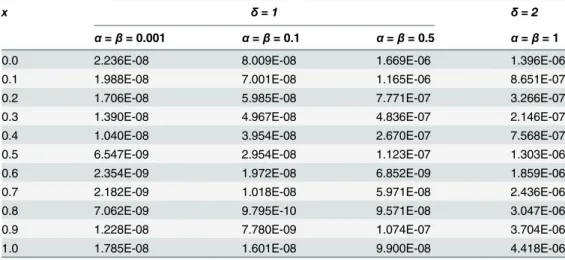
Table 4. The absolute errors for example 1 for different values ofα,β,δand for timet= 0.1.

x δ= 1 δ= 2

α=β= 0.001 α=β= 0.1 α=β= 0.5 α=β= 1

0.0 2.236E-08 8.009E-08 1.669E-06 1.396E-06

0.1 1.988E-08 7.001E-08 1.165E-06 8.651E-07

0.2 1.706E-08 5.985E-08 7.771E-07 3.266E-07

0.3 1.390E-08 4.967E-08 4.836E-07 2.146E-07

0.4 1.040E-08 3.954E-08 2.670E-07 7.568E-07

0.5 6.547E-09 2.954E-08 1.123E-07 1.303E-06

0.6 2.354E-09 1.972E-08 6.852E-09 1.859E-06

0.7 2.182E-09 1.018E-08 5.971E-08 2.436E-06

0.8 7.062E-09 9.795E-10 9.571E-08 3.047E-06

0.9 1.228E-08 7.780E-09 1.074E-07 3.704E-06

1.0 1.785E-08 1.601E-08 9.900E-08 4.418E-06

(9)

The approximate solution is obtained by the proposed scheme for three different values ofδ

= 1,2,3 in the domainx2(0,1) andt2(0,2)forδ= 1,2, and t2(0,5) forδ= 3.

We assume the solution is expressed by Exp-function method given byEquation (20). The

fitness function is developed for each value ofδwithβ= 0 andα= 1. For example, the fitness

function withδ= 3is given as follows

"_j¼ 1

121

X

11

i¼1

X

11

j¼1

ðou0ðkxjþotiÞ þu 3

kðkxjþotiÞu

0_ð

kxjþotiÞ k

2

u″ðkx_jþot_iÞÞ2

þ 1 11

X

11

j¼1

uðxj;0Þ 1

2þ 1

2tanh 3

8 xj

1

3

0

B @

1

C A

2

ð24Þ Table 5. Comparison of numerical solutions and absolute errors forα= 2,β= 5,δ= 3/2.

x t uexact u_(η) Absolute errors

0.1 0.2 0.881815 0.881912 9.65E-05

0.4 0.975295 0.975367 7.15E-05

0.6 0.995333 0.995292 4.15E-05

0.8 0.999137 0.999127 9.74E-06

1 0.999841 0.999874 3.31E-05

0.5 0.2 0.824570 0.824537 3.29E-05

0.4 0.960817 0.960883 6.64E-05

0.6 0.992485 0.992451 3.47E-05

0.8 0.998605 0.998579 2.69E-05

1 0.999743 0.999767 2.43E-05

1 0.2 0.727552 0.727337 2.15E-04

0.4 0.931343 0.931303 3.99E-05

0.6 0.986412 0.986394 1.83E-05

0.8 0.997463 0.997416 4.66E-05

1 0.999532 0.999540 8.35E-06

Table 6. Comparison of numerical solutions and absolute errors between the proposed scheme, OHAM[10] and ADM [11] forα=β= 0.001 and δ= 1.

Exact Proposed Absolute errors

x t uexact u_(η) Proposed ADM [11] OHAM [10]

0.1 0.001 0.499988 0.499988 1.97E-08 1.94E-06 2.25E-08

0.005 0.499989 0.499989 1.97E-08 9.69E-06 1.12E-07

0.01 0.499990 0.499990 1.97E-08 1.94E-06 2.25E-07

0.5 0.001 0.499938 0.499938 3.58E-09 1.94E-06 4.58E-08

0.005 0.499939 0.499939 3.71E-09 9.69E-06 2.29E-07

0.01 0.499940 0.499940 3.88E-09 1.94E-06 4.58E-07

0.9 0.001 0.499888 0.499888 1.80E-08 1.94E-06 4.58E-08

0.005 0.499889 0.499889 1.77E-08 9.69E-06 2.29E-07

0.01 0.499890 0.499890 1.74E-08 1.94E-06 4.58E-07

(10)

GA is used to solve the minimization problem such as given byEquation (24)and to obtain

the optimal values of unknown constants inEquation (20). The parameter settings for the

im-plementation of GA are given inTable 1.

The optimal values of unknown constants achieved by GA are given inTable 9for each

value ofδ= 1, 2, 3. The approximate solutions of generalized Burgers0_{equation are obtained}

consequently by using the values of unknown constants inEquation (20).

In Tables10–13we provide the comparison of numerical solutions obtained by the

pro-posed scheme with the exact solutions, and the solutions obtained by ADM [11] and CBRBF [13]. The comparisons of numerical solutions and absolute errors reveals that the proposed scheme is quite competent with other methods including ADM and RBF used in [11,13] for

solving the generalized Burgers0_{equation. The comparison further reveals that the proposed}

scheme is capable to achieve the approximate solutions in the larger domain of timetwith

greater accuracy. Moreover, forδ= 3 more accurate results are obtained by the proposed

scheme as compared to ADM [11] and CBRBF [13].

Table 7. Comparison of numerical solutions and absolute errors between the proposed scheme, OHAM [10] and ADM [11] forα=β= 1 andδ= 2.

Exact Proposed Absolute errors

x t uexact u_(η) Proposed ADM [11] OHAM [10]

0.1 0.0001 0.695266 0.695267 1.08E-06 2.80E-04 1.17E-05

0.0005 0.695426 0.695427 1.08E-06 1.40E-03 5.87E-05

0.001 0.695625 0.695626 1.08E-06 2.80E-03 1.17E-04

0.5 0.0001 0.646130 0.646129 1.14E-06 2.69E-04 5.33E-05

0.0005 0.646297 0.646296 1.14E-06 1.34E-03 1.06E-05

0.001 0.646506 0.646505 1.14E-06 2.69E-03 1.06E-05

0.9 0.0001 0.595310 0.595306 4.12E-06 2.55E-04 9.29E-06

0.0005 0.595481 0.595477 4.12E-06 1.27E-03 4.64E-05

0.001 0.595695 0.595691 4.12E-06 2.55E-03 9.29E-04

Table 8. Comparison of numerical solutions and absolute errors between the proposed scheme and HPM [12] forδ= 1 at different values ofα andβ.

α=β= 0.1 α=β= 0.5

Exact Proposed Absolute errors Exact Proposed Absolute errors

t x uexact u_(η) Exact Proposed uexact u_(η) Exact Proposed

0.1 0.2 0.500062 0.500062 5.98E-08 4.32E-08 0.501562 0.501562 7.77E-07 6.17E-08

0.4 0.497563 0.497562 3.95E-08 1.08E-07 0.489064 0.489064 2.67E-07 1.60E-05

0.6 0.495063 0.495063 1.97E-08 1.74E-07 0.476580 0.476580 6.85E-09 2.58E-05

0.8 0.492563 0.492563 9.80E-10 2.40E-07 0.464124 0.464124 9.57E-08 3.54E-05

0.4 0.2 0.507749 0.507749 6.75E-08 3.85E-07 0.543639 0.543631 7.40E-06 7.87E-05

0.4 0.505250 0.505250 4.89E-08 6.65E-07 0.531209 0.531205 4.69E-06 7.89E-05

0.6 0.502750 0.502750 2.93E-08 1.71E-06 0.518741 0.518738 2.95E-06 2.36E-04

0.8 0.500250 0.500250 9.08E-09 2.76E-06 0.506250 0.506248 1.87E-06 3.92E-04

0.8 0.2 0.517992 0.517992 5.09E-08 7.28E-06 0.598688 0.598635 5.22E-05 1.24E-03

0.4 0.515495 0.515495 4.27E-08 3.08E-06 0.586618 0.586583 3.48E-05 6.22E-04

0.6 0.512997 0.512997 3.09E-08 1.12E-06 0.574443 0.574419 2.32E-05 2.80E-06

0.8 0.510498 0.510498 1.63E-08 5.32E-06 0.562177 0.562161 1.54E-05 6.28E-04

(11)

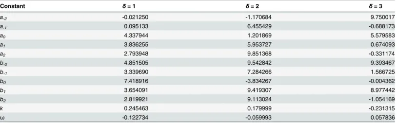
Table 9. Optimal values of unknown constants acquired by GA for example 2 for different values ofδ.

Constant δ= 1 δ= 2 δ= 3

a_-2 -0.021250 -1.170684 9.750017

a_-1 0.095133 6.455429 -0.688173

a0 4.337944 1.201869 5.579583

a1 3.836255 5.953727 0.674093

a2 2.793948 9.851368 -0.331174

b_-2 4.851505 9.542842 9.393467

b_-1 3.339690 7.284266 1.566725

b0 7.418916 -3.834267 -0.004362

b1 3.654091 9.419307 8.977442

b2 2.819921 9.113024 -1.054169

k _0.245463 _0.179999 _-0.231315

ω -0.122734 -0.059993 0.057836

Table 10. Numerical solutions of generalized Burgers0_{equation by the proposed scheme and comparison with exact solutions, ADM [}₁₁_{], and}

RBF [13] forβ= 0,α= 1, andδ= 1.

Exact Proposed ADM CBRBF Absolute errors

t x uexact u_(η) [11] [13] Proposed ADM CBRBF

0.5 0.1 0.518741 0.518740 0.518741 0.518739 1.14E-07 6.34E-08 2.00E-06

0.5 0.468791 0.468791 0.468791 0.468790 1.13E-07 5.66E-08 1.00E-06

0.9 0.419458 0.419459 0.419458 0.419449 1.56E-06 4.12E-08 9.00E-06

1.0 0.1 0.549834 0.549833 0.549832 0.549831 1.17E-06 2.02E-06 3.00E-06

0.5 0.500000 0.499999 0.499998 0.499998 3.79E-08 1.84E-06 2.00E-06

0.9 0.450166 0.450167 0.450165 0.450157 1.28E-06 1.37E-06 9.00E-06

2.0 0.1 0.610639 0.610638 0.610575 0.610635 8.44E-07 6.42E-05 4.00E-06

0.5 0.562177 0.562176 0.562116 0.562175 1.16E-07 6.06E-05 2.00E-06

0.9 0.512497 0.512498 0.512450 0.512488 9.72E-07 4.75E-05 9.00E-06

CBRBF [13] forβ= 0,α= 1, andδ= 2.

0.5 0.1 0.714919 0.714918 0.714919 0.714920 7.43E-07 1.25E-08 1.00E-06

0.5 0.666837 0.666836 0.666837 0.666839 1.16E-06 1.49E-08 2.00E-06

0.9 0.616567 0.616565 0.616567 0.616567 2.38E-06 1.39E-08

-1.0 0.1 0.734037 0.734034 0.734037 0.734037 2.94E-06 1.25E-08

-0.5 0.687205 0.687202 0.687205 0.687206 3.22E-06 4.75E-07 1.00E-06

0.9 0.637701 0.637697 0.637701 0.637699 4.20E-06 4.39E-07 2.00E-06

2.0 0.1 0.770284 0.770277 0.770272 0.770286 7.21E-06 1.18E-05 2.00E-06

0.5 0.726464 0.726456 0.726449 0.726469 7.35E-06 1.49E-05 5.00E-06

0.9 0.679109 0.679101 0.679095 0.679110 8.03E-06 1.43E-05 1.00E-06

(12)

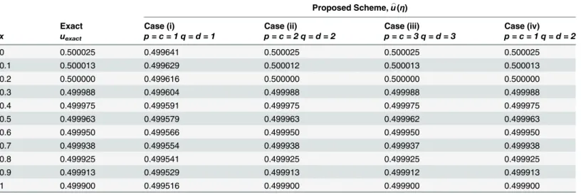
Finally, we study the effect of change in the values ofcanddinEquation (9)on the accuracy of approximate solution, and show the reliability of the proposed scheme. We used following test cases

Case (i)p = c = 1 q = d = 1

Case (ii)p = c = 2 q = d = 2

Case (iii)p = c = 3 q = d = 3

Case (iv)p = c = 1 q = d = 2

We consider the generalized Burgers0_-Fisher_{Equation (1)}_with_α₌_β_{= 0.001, and}_δ_{= 1. The}

approximate solution is obtained in the domainx2(0,1) andt2(0,1). GA has been used with

the same settings for all the four cases (i)—(iv) as prescribed inTable 1for example 1, except

with a change in chromosome size for each case which is 8, 12, 16, and 10 for case(i), case(ii), case (ii), and case(iv) respectively. The approximate solutions have been obtained for each case

and absolute errors have been computed. InTable 14we provide the approximate solution

ob-tained by the proposed scheme for each case at timet = 0.1.Table 15shows average absolute

er-rors obtained by the proposed scheme for each case (i)—(iv) fort2(0,1), also computational

Table 13. Numerical solutions of generalized Burgers0_{equation by the proposed scheme and comparison with exact solutions, and CBRBF [}₁₃_]

forα= 1,β= 0, andδ= 3.

Exact Proposed CBRBF Absolute errors

t x uexact u_(η) [13] Proposed CBRBF

0.5 0.1 0.796173 0.796174 0.796176 1.00E-06 3.00E-06

0.5 0.75487 0.754871 0.754877 1.00E-06 7.00E-06

0.9 0.710485 0.710486 0.710486 1.00E-06 1.00E-06

1.0 0.1 0.808297 0.808299 0.808299 2.00E-06 2.00E-06

0.5 0.768157 0.768159 0.768165 2.00E-06 8.00E-06

0.9 0.724622 0.724625 0.724623 3.00E-06 1.00E-06

2.0 0.1 0.831283 0.831288 0.831286 5.00E-06 3.00E-06

0.5 0.793701 0.793706 0.793709 5.00E-06 8.00E-06

0.9 0.752176 0.752182 0.752177 6.00E-06 1.00E-06

5.0 0.1 0.889248 0.88926 0.889252 1.20E-05 4.00E-06

0.5 0.860439 0.860452 0.860452 1.30E-05 1.30E-05

0.9 0.826825 0.826839 0.826828 1.40E-05 3.00E-06

CBRBF[13] for,α= 1,β= 0, andδ= 3.

0.0001 0.1 0.783660 0.783659 0.784106 - 4.55E-07 4.46E-04

-0.5 0.741285 0.741285 0.743145 - 5.66E-07 1.86E-03

-0.9 0.696157 0.696158 0.697089 - 7.00E-07 9.32E-04

-0.0005 0.1 0.783670 0.783670 0.784115 0.783664 4.57E-07 4.45E-04 6.00E-06

0.5 0.741296 0.741296 0.743150 0.741291 5.63E-07 1.85E-03 5.00E-06

0.9 0.696169 0.696170 0.697089 0.696165 6.98E-07 9.20E-04 4.00E-06

0.001 0.1 0.783683 0.783682 0.784127 0.783664 4.60E-07 4.44E-04 1.90E-05

0.5 0.741309 0.741309 0.743157 0.741293 5.61E-07 1.85E-03 1.60E-05

0.9 0.696183 0.696184 0.697088 0.696168 6.95E-07 9.05E-04 1.50E-05

(13)

time and number of generations utilized are given for the sake of comparison. From the

com-parison ofTable 15, it is observed that the average absolute error corresponding to case(i) with

p = c = 1andd = q = 1is relatively very high compared to other cases (ii)–(iv). It is also

ob-served that the accuracy is fairly equal for the remaining cases (ii)—(iv), however the

computa-tional time is quite different. It can be seen fromTable 14that for case (iv) we get the average

absolute error fairly comparable to cases (ii) and (iii), but with lesser number generations and smaller computational time. Therefore it can be concluded on the basis of the simulation

re-sults that the choice ofc,dhave influence on the accuracy of approximate solutions and

computational time. Nonetheless the comparison clearly demonstrates the accuracy and reli-ability of the proposed scheme.

Conclusions

A simple straightforward heuristic scheme based on the hybridization of Exp-function method and evolutionary algorithm has been proposed for obtaining the numerical solution of NPDEs. The proposed scheme has been successfully implemented for obtaining the numerical solutions

of the generalized Burgers0_{-Fisher and Burgers}0_{equations. From the comparisons of numerical}

solutions made with the exact solutions, and some traditional methods including ADM, HPM, OHAM, and CBRBF, it can be concluded that the proposed scheme is effective and viable for solving such problems. Moreover, the beauty of the proposed scheme is that it can provide the approximate solution of the given NPDE on continuous values of time in the solution domain, once the unknown parameters are achieved.

Table 14. Comparison of approximate solutions with different values ofcanddatt = 0.1.

Proposed Scheme,u_(η)

Exact Case (i) Case (ii) Case (iii) Case (iv)

x uexact p = c = 1 q = d = 1 p = c = 2 q = d = 2 p = c = 3 q = d = 3 p = c = 1 q = d = 2

0 0.500025 0.499641 0.500025 0.500025 0.500025

0.1 0.500013 0.499629 0.500012 0.500013 0.500013

0.2 0.500000 0.499616 0.500000 0.500000 0.500000

0.3 0.499988 0.499604 0.499988 0.499988 0.499988

0.4 0.499975 0.499591 0.499975 0.499975 0.499975

0.5 0.499963 0.499579 0.499963 0.499962 0.499963

0.6 0.499950 0.499566 0.499950 0.499950 0.499950

0.7 0.499938 0.499554 0.499938 0.499937 0.499938

0.8 0.499925 0.499541 0.499925 0.499925 0.499925

0.9 0.499913 0.499529 0.499913 0.499912 0.499913

1 0.499900 0.499516 0.499900 0.499900 0.499900

Table 15. Effect of change incanddon the accuracy and computational time of the proposed scheme.

Values ofp,q,c,d Average absolute error No. of generations Computational time in sec

Case (i):p = c = 1q = d = 1 1.91E-03 196 80

Case (ii):p = c = 2 q = d = 2 1.97E-07 457 177

Case (iii):p = c = 3 q = d = 3 1.42E-07 279 97

Case (iv):p = c = 1 q = d = 2 1.76E-07 51 40

(14)

Author Contributions

Conceived and designed the experiments: SAM IQM. Performed the experiments: SAM. Ana-lyzed the data: SAM IMQ MA ANM IH. Contributed reagents/materials/analysis tools: SAM MA IH. Wrote the paper: SAM. Read and polished the paper: SAM IMQ ANM MA IH.

References

1. Jiwari R (2012) Quasilinearization approach for numerical simulation of Burgers' equation. Computer Physics Communications 183: 2413–2423.

2. Jiwari R, Mittal RC, Sharma KK (2013) A numerical scheme based on weighted average differential quadrature method for the numerical solution of Burgers' equation. Applied Mathematics and Computa-tion 219: 6680–6691.

3. Mittal RC, Jiwari R, Sharma KK (2013) A numerical scheme based on differential quadrature method to solve time dependent Burgers' equation. Engineering Computations 30 (1): 117–131.

4. Mittal RC, Jiwari Ram (2012) A differential quadrature method for solving Burgers'-type equation. Inter-national Journal of Numerical Methods for Heat and Fluid Flow 22 (7): 880–895.

5. Mittal RC, Jiwari R (2009) Study of Burger-Huxley Equation by Differential Quadrature Method. Interna-tional Journal od Applied Mathematics and Mechanics 5(8): 1–9.

6. Mittal RC, Jiwar R (2009) Differential Quadrature Method for Two Dimensional Burgers' Equations. In-ternational Journal of Computational Methods in Engineering Science and Mechanics 10: 450–459. 7. Jiwari R, Pandit S, Mittal RC (2012) Numerical simulation of two-dimensional sine-Gordon solitons by

differential quadrature method. Computer Physics Communications 183: 600–616.

8. Mittal RC, Tripathi A (2014) Numerical solutions of generalized Burgers—Fisher and generalized Bur-gers—Huxley equations using collocation of cubic B-splines.International Journal of Computer Mathe-maticshttp://dx.doi.org/10.1080/00207160.2014.920834.

9. Kheiri H, Ebadi DG (2010) Application of the (G0_{/G)-expansion method for the Burgers, Fisher, and}

Bur-gers-Fisher equations, Acta Universitatis Apulensis 24: 35–44.

10. Nawaz R, Ullah H, Islam S, Idrees M (2013) Application of optimal homotopy asymptotic method to Bur-ger equations. Journal of Applied Mathematicshttp://dx.doi.org/10.1155/2013/387478doi:10.1155/ 2013/935154PMID:24415902

11. Ismail HNA, Raslan K, Abd Rabboh AA (2004) Adomian decomposition method for Burger’s—Huxley and Burger’s—Fisher equations. Applied Mathematics and Computation 159: 291–301.

12. Rashidi MM, Ganji DD, Dinarvand S (2009) Explicit analytical solutions of the generalized Burger and Burger—Fisher equations by homotopy perturbation method. Numerical Methods for Partial Differential Equations 25: 409–417. doi:10.1002/num.20350

13. Khattak AJ (2009) A computational meshless method for the generalized Burger’s—Huxley equation. Applied Mathematical Modelling 33: 3718–3729.

14. Javidi M (2006) Modified pseudospectral method for generalized Burger’s-Fisher equation. Internation-al MathematicInternation-al Forum 1(32): 1555–1564.

15. Behzadi SS (2011) Numerical solution for solving Burger’s-Fisher equation by iterative methods. Math-ematical and Computational Applications 6(2): 443–455.

16. Moghimi M, Hejazi FSA (2007) Variational iteration method for solving generalized Burger—Fisher and Burger equations. Chaos, Solitons and Fractals 33: 1756–1761.

17. Sari M (2011) Differential quadrature solutions of the generalized Burgers-Fisher equation with a strong stability preserving high-order time integration. Mathematical and Computational Applications 16(2): 477–486.

18. He JH, Wu XH (2006) Exp-function method for nonlinear wave equations. Chaos, Solitons and Fractals 30: 700–708.

19. Xu ZH, Xian DQ (2010) Application of Exp-function method to generalized Burgers-Fisher equation. Acta Mathematicae Applicatae Sinica, English Series 26(4): 669–676. doi:10.1007/s10255-010-0031-0 20. ÖzişT, Köroğlu C (2008) A novel approach for solving the Fisher equation using Exp-function method.

Physics Letters A 372: 3836–3840.

21. Chun C. (2008) Application of Exp-function method to the generalized Burgers-Huxley equation. Jour-nal of Physics 96: 012217. doi:10.1088/1742-6596/96/1/012217

(15)

23. Hu M, Jia Z, Chen Q, Jia S (2014) Exact solutions for nonlinear wave equations by the Exp-function method. Abstract and Applied Analysis: doi:10.1155/2014/252168

24. Assas LMB (2009) New exact solutions for the Kawahara equation using Exp-function method. Journal of Computational and Applied Mathematics 233: 97–102.

25. Malik SA, Qureshi IM, Amir M, Haq I (2014) Numerical solution to nonlinear biochemical reaction model using hybrid polynomial basis differential evolution technique. Advanced Studies in Biology 6(3): 99–113. doi:10.12988/asb.2014.4520

26. Malik SA, Qureshi IM, Amir M, Haq I (2014) Nature inspired computational technique for the numerical solution of nonlinear singular boundary value problems arising in physiology. The Scientific World Jour-nal: doi:10.1155/2014/837021

27. Khan JA, Raja MAZ, Qureshi IM (2011) Novel approach for a van der pol oscillator in the continuous time domain. Chinese Physics Letters 28 (11): 110205.

28. Arqub OA, Abo-Hammour Z, Momani S, Shawagfeh N (2012) Solving singular two-point boundary value problems using continuous genetic algorithm. Abstract and Applied Analysis: doi:10.1155/2012/ 205391

29. Caetano C, Reis JL Jr, Amorim J, Lemes MR, Pino AD Jr (2011) Using neural networks to solve nonlin-ear differential equations in atomic and molecular physics. International Journal of Quantum Chemistry 111: 2732–2740.

30. Malik SA, Qureshi IM, Zubair M, Haq I (2012) Solution to force-free and forced duffing-van der pol oscil-lator using memetic computing. Journal of Basic and Applied Scientific Research 2(11): 11136–11148. 31. Malik SA, Qureshi IM, Zubair M, Amir M (2013) Numerical solution to Troesch’s problem using hybrid

heuristic computing. Journal of Basic and Applied Scientific Research 3(7): 10–16.

32. Malik SA, Qureshi IM, Zubair M, Amir M (2013) Hybrid heuristic computational approach to the Bratu problem. Research Journal of Recent Sciences 2(10): 1–8.

33. Malek A, Beidokhti RS (2006) Numerical solution for high order differential equations using a hybrid neural network—optimization method. Applied Mathematics and Computation 183: 260–271. 34. Raja MAZ, Khan JA, Qureshi IM (2011) A new stochastic approach for solution of Riccati differential

equation of fractional order. Annals of Mathematics and Artificial Inteigence: doi: 10.1007/s10472-010-9222-x

35. Behrang MA, Ghalambaz M, Assareh E, Noghrehabadi AR (2011) A New Solution for Natural Convec-tion of Darcian Fluid about a Vertical Full Cone Embedded in Porous Media Prescribed Wall Tempera-ture by using a Hybrid Neural Network-Particle Swarm Optimization Method. World Academy of Science, Engineering, and Technology 49: 1098–1103.

36. Mitchell M (1995) Genetic algorithms: an overview. Complexity 1 (1): 31–39.