Improved hyperbolic function method and exact solutions for variable coefficient Benjamin-Bona-Mahony-Burgers equation

IMPROVED HYPERBOLIC FUNCTION METHOD

AND EXACT SOLUTIONS FOR VARIABLE COEFFICIENT

BENJAMIN-BONA-MAHONY-BURGERS EQUATION

by

Hong-Cai MAa,b*_{, Xiao-Fang PENG}a_{, and Dan-Dan YAO}a a

Department of Applied Mathematics, Donghua University, Shanghai, China b

Department of Mathematics and Statistics, University of South Florida, Tampa, Fla., USA

Original scientific paper DOI: 10.2298/TSCI1504183M

By using the improved hyperbolic function method, we investigate the variable coefficient Benjamin-Bona-Mahony-Burgers equation which is very important in fluid mechanics. Some exact solutions are obtained. Under some conditions, the periodic wave leads to the kink-like wave.

Key words: Benjamin-Bona-Mahony-Burgers equation, exact solutions, hyperbolic function method

Introduction

Nowadays, non-linear partial differential equations (NLPDE) are becoming more and more important, especially their broad applications on modeling many physical phenom-ena. For instance, solid state physics, fluid mechanics, and so on [1]. It is very valuable to do some research on how to solve NLPDE exact solutions and investigate the property of the so-lutions.

The Benjamin-Bona-Mahony-Burgers (BBMB) equation:

0 t xxt xx x x

u −u −αu +uu +u =

is proposed as a model to study the unidirectional long waves of small amplitudes in water, which is an alternative to the KdV equation [2].

In this paper we will study the variable coefficient BBMB equation:

( ) ( ) ( ) ( ) 0

t xxt xx x x

u −λ t u −α t u +β t uu +γ t u =

where ( ),λ t α( ),t β( ), and ( )t γ t are arbitrary time-dependent coefficients.

If α(t) = 0, λ(t) = 1, and (t) = 1, eq. (1) is an alternative to the regularized long wave equation proposed by Benjamin et al. [3] and Peregrine [4]. The variable coefficient BBMB eq. (1) [5] is proposed to describe long waves of small amplitudes broadcasting in non-linear dispersive media. This model has been introduced [6], which plays a very important role in mathematics and fluid. During the past few years, numerous methods in solving BBMB equa-tions have been discovered by many authors, such as G'/G method, homotopy analysis meth-od, He' methmeth-od, etc. [7, 8].

––––––––––––––

Hyperbolic function method was first proposed in [9], which is based on the fact that most solitary wave solutions have form of hyperbolic function. This method has been used to find the exact solutions of many non-linear wave equations, such as Burgers' equation, KdV equation, etc. [9, 10].

Improved hyperbolic function method

For partial differential equation (PDE) of two independent variables x, t:

P ( ,t x u, _x, u_t, u_xx, ...)=0 (2)

we consider its traveling wave solution of the form:

( , )u x t =ϕ ξ( ), ξ =k x( )+c(t)+l

where k(x)and c(t)are functions of single variable.

By using this traveling wave transaction, we can change non-linear PDE eq. (2) to a variable coefficient differential equation (VCDE).

Supposing that the solution of this VCDE is:

1

0 1

( ) m _i i m _j j

i j

a f b f g

φ ξ −

= =

=∑ + ∑ (4)

where

1 sinh

,

cosh cosh

f g

r r

ξ

ξ ξ

= =

+ + (5)

and ai, bj, and r are coefficients to be determined. m can be determined by balancing [11] the

highest order derivatives and highest order non-linear terms appearing in VCDE, what's more:

2 2 2 2

, 1 , 1 2 ( 1)

f_ξ = −fg g_ξ = −g −rf g = − rf + r − f (6)

By substituting eq. (4) into eq. (2), and using eq. (5) to simplify the VCDE until it only involves exponential term of f and g (the degree of g is less than 1). Then combining the similar terms of f and g, we will establish a set of equation. By solving this set of equation, the exact solution of eq. (2) will be obtained.

Obtain exact solution of BBMB equation by improved hyperbolic function method

Firstly, we consider the following transformations:

( , )u x t =ϕ ξ( ), ξ =k x( )+c t( )+l (7)

where ( ),k x c t( )are arbitrary functions.

Substituting eq. (7) into eq. (1) we have the equation:

2

[ ( )c t′ −α( ) ( )t k x′′ +γ(t)]ϕ ξ′( ) [ ( ) ( )− λ t c t k x′ ′′( )+α( )t k ′( )]x ϕ ξ′′( )+

2

( ) ( ) ( ) ( )t k x ( ) ( )t c t k ( )x ( ) 0

β ′ ϕ ξ ξ′ λ ′ ′ ϕ ξ′′′

+ − = (8)

0 1 1

( ) a a f b g

φ ξ = + +   (9)

By substituting eq. (9) into eq. (8), simplifying the eq. (8) until it only involves ex-ponential term of f and g (the degree of g is less than 1), by supposing their coefficient equal to zero, we obtain the system:

2 1

2

1 1 1 1 1

2 2 2

1 1 1 1 0 0

1 1

(1) ( 1)( 1) ( ) ( ) ( ) 0

(2) ( 1)( 1){ ( ) ( ) "( ) ( ) ( ) [ ( ) 12 ( ) ( )] ( )} 0

(3) [3 ( ) ( ) (1 ) ( )] ( ) [(3 ) ( ) (1 ) ( )] ( )

[3 ( )

b r r t c t k x

r r a t c t k x a b t k x a t b r t c t k x

a r t c t b r t k x b a r a a r t r t k x

a r t b

λ

λ α λ

λ α β γ

α ′ ′ + − = ′ ′ ′′ ′ ′ + − + + + = ′ − − ′′ + + − + − ′ +

+ + 2 2 2

1

1 1 1 0 1 1 1 1

2

1 1 1

2

1 1 1 0 1

(7 4) ( ) ( )] ( ) (1 ) ( ) 0

(4) [ ( ) ( ) ( ) ( )] ( ) [ ( ) ( ) ( )] ( )

[ ( ) ( ) ( )] ( ) ( ) 0

(5) [ ( ) ( ) ( )] ( ) [( ) ( )

r t c t k x b r c t

b rc t b r t a t c t k x a rb t a b t b r t k x

a t b r t c t k x b rc t

b r t c t a t k x b r a a t

λ

α λ β β γ

α λ

λ α β

′ ′ ′ − + − = ′ − − ′ ′′ + − + ′ − ′ ′ ′ − + + =

′ + ′′ + − − ₁

2

1 1 1

2 2 2 2 2

1 1 1 1

2 2

1 1

2 1

( )] ( )

[ ( ) ( ) ( )] ( ) ( ) 0

(6) 2 ( 1) ( ) ( ) ( ) ( ) ( ) ( )

[2 ( 1) ( ) 6 ( ) ( )] ( ) 0

(7) ( 1)( 1) ( ) ( ) ( ) 0

a t k x

a t c t b r t k x a c t

b r t c t k x b b r a t k x

b r t a r t c t k x

a r r t c t k x

γ γ α λ β α λ λ ⎧ ⎪ ⎪ ⎪ ⎪ ⎪ ⎪ ⎪ ⎪ ⎪ ⎨ ⎪ _{′ +} ⎪ ⎪ _{+ ′ + ′ − ′ =} ⎪ ⎪ _{− ′ ′′ − − − ′ +} ⎪ ⎪ _{+ − + ′ ′ =} ⎪ ⎪ _{+ − ′ ′ =} ⎩

Solving this system by Maple gives the following results:

λ

1 ( )

( ) ( ) b t k x t β α −

′ = (10)

2

1 ( 1) 1

a = ± r − b (11)

2 1 ( ) ( ) 0 1 ( )

( )

( )

b t t a b t

c t

t

γ β β

α

+

′ = (12)

Equation (10) indicates that ( )/ ( )β t α t must be a constant:

1 1 1 1 1 0

( )t c ( ),t k x( ) b c, c t( ) b c[ ( )t a ( )]t

β = α ′ = − ′ = γ + β

We obtain the solution of variable coefficient BBMB eq. (1):

2

1 1

0

1 sinh[ ( ) ( ) ]

( , )

cosh[ ( ) ( ) ] cosh[ ( ) ( ) ]

b r b k x c t l

u x t a

r k x c t l r k x c t l

− + +

= ± +

+ + + + + +

where

1 1 1 1 0

( ) , ( ) [ ( ) ( )]d

k x = −b c x c t =b c

∫

Figure 1 shows a special solution of eq. (1), when we suppose that:

0 1, 1 1 2, 0,

( ) cos , ( ) sin

a b c r l

t t t t

γ β

= = = = =

= =

From the figure we can see that the wave is a kind of kink-like wave and the am-plitude is constant in the process of transmis-sion. Since (t) and (t) are time dependent periodic function, wave velocity (both size and direction) periodically changes over time.

(2) When a1 = r = 0, we have:

1 ( )

( )

2 ( )

b t

k x

t β α

′ = − (14)

2 1 ( ) ( ) 0 1 ( )

( )

2 ( )

b t t a b t

c t

t

γ β β

α

+

′ =

Equation (14) indicates that (t)/α(t) must be a constant. Then, we have:

1 1

2 2 0

( ) , ( ) [ ( ) ( )]d

2 2

b b

k x = − c x c t = c

∫

The solution of variable coefficient BBMB equation eq. (1) is:

1 0

sinh[ ( ) ( ) ] ( , )

cosh[ ( ) ( ) ]

b k x c t l

u x t a

r k x c t l

+ +

= +

+ + + (16)

where

1 2

1

2 0

( ) 2

( ) [ ( ) ( )]d

2

b

k x c x

b

c t c γ t a β t t

= −

=

_∫

and a0, b1, and c2 are constants.

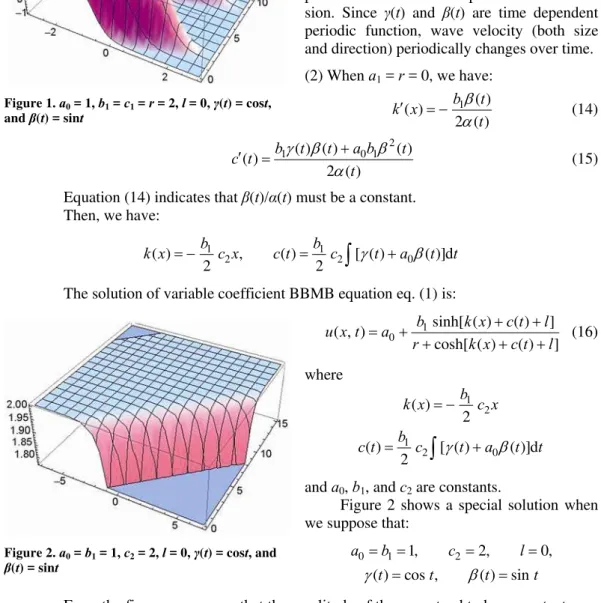
Figure 2 shows a special solution when we suppose that:

0 1 1, 2 2, 0,

( ) cos , ( ) sin

a b c l

t t t t

γ β

= = = =

= =

From the figure we can see that the amplitude of the wave tend to be a constant over time in the process of transmission.

Conclusions

In this article, the improved hyperbolic function method is utilized to find the solu-tions of the variable coefficient BBMB equation. It is very important in fluid mechanics. As we Figure 1. a_{0 = 1,} b_{1 =} c_{1 =} r _{= 2,} l _{= 0,} Ȗ₍t_{) = cos}t_,

and ȕ(t_{) = sin}t

know, hyperbolic function method is an effective method in solving non-linear partial differ-ential equations. We also indicate that hyperbolic function method is a strong method not only in solving constant coefficient non-linear partial differential equations but also in solving var-iable coefficient non-linear partial differential equations.

Acknowledgments

The work is in part supported by the National Natural Science Foundation of China (project No.11371086), the Fund of Science and Technology Commission of Shanghai Mu-nicipality (project No.ZX201307000014) and the Fundamental Research Funds for the Cen-tral Universities.

References

[1] Zhang, P., Lin, F. H., Lectures on the Analysis of Non-Linear Partial Differential Equations, Higher Ed-ucation Press, Beijing, China, 2013

[2] Bona, J. L., Smith, R., The Initial-Value Problem for the Korteweg-de Vries Equation, Philosophical Transactions of the Royal Society of London Series A, 278 (1975), 1287, pp. 555-601

[3] Benjamin, T. B., et al., Model Equations for Long Waves in Non-Linear Dispersive Systems, Philosoph-ical Transactions of the Royal Society of London Series A, 272 (1972), 1220, pp. 47-78

[4] Peregrine, D. H., Calculations of the Development of an Under Bore, Journal of Fluid Mechanics, 25

(1966), 2, pp. 321-326

[5] Mei, M., Large-Time Behavior of Solution for Generalized Benjamin-Bona-Mahony-Burgers Equations,

Non-Linear Analysis, 33 (1998), 7, pp. 699-714

[6] Kumar, V., et al., Painleve Analysis, Lie Symmetries and Exact Solutions for Variable Coefficients Ben-jamin-Bona-Mahony-Burger (BBMB) Equation, Communications in Theoretical Physics, 60 (2013), 2, pp. 175-182

[7] Tari, H., Ganji, D. D., Approximate Explicit Solutions of Non-Linear BBMB Equation by He's Methods and Comparison with the Exact Solution, Physics Letters A, 367 (2007), 1, pp. 95-101

[8] Kadri, T., et al., Methods for the Numerical Solution of the Benjamin-Bona-Mahony-Burgers Equation,

Numer. Math. Partial. Diff. Eq., 24 (2008), 6, pp. 1501-1516

[9] Shi, Y., et al., Exact Solutions of Generalized Burgers' Equation with Variable Coefficients, East China Normal University Transaction, 5 (2006), pp. 27-34

[10]Shi, Y. R., et al., Exact Solutions of Variable Coefficients Burgers' Equations, Journal of Lanzhou Uni-versity (Natural Sciences), 41 (2005), 2, pp. 107-112

[11]Wang, M., et al., Application of a Homogeneous Balance Method to Exact Solutions of Non-Linear Equations in Mathematical Physics, Physics Letters A, 216 (1996), 1, pp. 67-75