ISSN 0101-8205 / ISSN 1807-0302 (Online) www.scielo.br/cam
Piecewise constant bounds for the solution of
nonlinear Volterra-Fredholm integral equations
S. YAZDANI and M. HADIZADEH∗
Department of Mathematics, K.N. Toosi University of Technology, P.O. Box 16315-1618, Tehran, Iran
E-mails: [email protected] / [email protected]
Abstract. In this paper, we compute piecewise constant bounds on the solution of mixed nonlinear Volterra-Fredholm integral equations. The enclosures are in the form of intervals which are guaranteed to contain the exact solution considering all round-off and truncation errors, so the width of interval solutions allows us to control the error estimation. An iterative algorithm to improve the accuracy of initial enclosures is given and its convergence are also investigated. Our numerical experiments show that the precision of interval solutions are reasonable in comparison to the classical methods and the obtained conditions and initial enclosure of the proposed algorithm are not restrictive.
Mathematical subject classification: 65G20, 45G10, 65G40.
Key words: Volterra-Fredholm integral equations, enclosure methods, interval analysis, guaranteed error bounds.
1 Introduction
During the last three decades, the role of enclosure methods in numerical solution of operator equations has continuously increased. In many cases computers are not perfect tools in scientific calculations, specially when using floating point arithmetic, the solutions are affected by rounding errors and this may led to completely wrong results (see e.g. [17]). This is more important when increasing
the speed of computers and for complicated equations, but its impossible to verify the accuracy of the results by classical schemes. Interval enclosure methods are able to compute guaranteed error bounds including all discretization and round-off errors in the computation. These methods are used in many applied areas e.g. fuzzy set theory, engineering problems with interval valued parameters or interval initial values, robust control, robotics, multimedia architectures [12], economics, beam physics, global optimization, signal processing and computer graphics [11] (see also [1] for a survey on enclosure methods).
Here, we restrict our attention to the computation of guaranteed bounds for the solution of the following nonlinear Volterra-Fredholm integral equation of mixed type
u(x,t) = f(x,t)+
Z t
0
Z
k(x,t, ξ, τ,u(ξ, τ ))dξdτ,
(x,t)∈ [0, χ] ×,
(1.1)
whereu(x,t)is an unknown function, and f(x,t)andk(x,t, ξ, τ,u(ξ, τ ))are known analytic functions defined on
D := [0, χ] × and S×R
(where S := {(x,t, ξ, τ ): 0 ≤ τ ≤ t ≤ χ;(x, ξ ) ∈ ×}), with k(x,t, ξ, τ,u)nonlinear inu andis closed subset ofRd(d =1,2,3).
These equations play an important role for abstract formulation of many ini-tial or boundary value problems of perturbed differenini-tial equations, nonlinear parabolic partial differential equations and partial integro-differential equations which arise in various applications like the mathematical modeling of chemical reaction kinetics, population dynamics [25], heat-flow in material with memory, electromagnetics [10], viscoelastic and reaction diffusion problems.
[2, 16], Euler Nystrom and trapezoidal Nystrom methods [13], the Adomian de-composition method [18], the time-stepping methods by a certain choice of direct quadrature (DQ) [3] and Sinc collocation method based on DE transformation in [14]. Generally, all of these classical methods are efficient and effective, but in many cases most of them are unable to control the truncation and round off errors in numerical computations. Here, our aim is to use an interval scheme which considers such these apparent errors.
As we know, there are not any considerable interval based works in solving mixed Volterra-Fredholm integral equations. Moore [19] has introduced an iter-ative algorithm for nonlinear integral equations based on the definition of interval integration. Caprani et al. [5] and Dobner [9] proposed several papers on solv-ing Fredholm integral equations ussolv-ing enclosure methods. Recently, Murashige and Oishi [21] presented numerical verification of solutions of periodic integral equations with a singular kernel and Nekrasov’s integral equation. In compar-ison to Fredholm type, there are a few enclosure methods on solving Volterra integral equations especially in the nonlinear form [8, 15].
In the present work, we propose an algorithm to provide piecewise constant bounds for the solution of nonlinear Volterra-Fredholm integral equations. Our algorithm is based on the early idea of Moore [19] for Volterra integral equa-tions. The organization of this paper is as follows: In section 2, we give basic notation, definitions and a summary on the principles of interval arithmetic. A new enclosure is constructed from an initial bound and its properties are studied in section 3 and then an iterative algorithm for the computation of piecewise constant bounds including its convergence conditions is presented. Finally, nu-merical experiments and a full discussion on initial enclosure, the algorithm conditions and also the number of iterations are reported to clarify the efficiency of the method.
2 Notations and auxiliary results of the interval theory 2.1 Interval arithmetic
We first introduce some basic properties of interval arithmetic from [20, 22, 23]. The set of compact real intervals is denoted by
Through out of this paper, using the notation of [23], intervals are denoted by boldface and lowercase letters are used for denoting scalars and vectors. A real numberx is identified with a point intervalx = [x,x]. The quality of interval analysis is measured by the width of the interval results, and a sharp enclosure for the exact solution is desirable. Themidpointand thewidth of an intervalx
are denoted by
m(x):=(x +x)/2 and w(x):= x−x,
respectively. The width of an interval vectorx = (x1, . . . ,xn)is the largest of
the widths of any of its component intervals
w(x)=maxw(xi), i=1, . . . ,n.
Considering|x| =max{|x|,|x|}, for anyx,y ∈ IRanda,b ∈R, we get the following properties:
w(ax+by)= |a|w(x)+ |b|w(y), (2.1)
w(xy)≤ |x|w(y)+ |y|w(x). (2.2) The four elementary operations of real arithmetic can be extended to intervals. Operations over intervals⋄ ∈ {+,−,∗, /}are defined by the general rule
x⋄y=x⋄y|x ∈x,y ∈y .
It is easy to see that the set of all possible results when applying an operator⋄ toxandy, forms a closed interval (for 0∈/yin the case of division) and the end point can be calculated by
x⋄y=min(x⋄y),max(x⋄y) , for ⋄ ∈ {+,−,∗, /}.
The following lemma gives an important property which is used frequently in this paper:
Lemma 1. Letk = [k,k]andy = [0,y], also there exists a constantα >1, such that|k| ≤αw(k), then
Proof. We consider the following three cases:
Case 1. If k ≤0≤k, thenw(ky)=w([k y,k y])=y(k−k)≤αw(k)y.
Case 2. If k ≤k ≤0, thenw(ky)=w([k y,0])= |k|y ≤ |k|y ≤αw(k)y.
Case 3. If 0 ≤ k ≤ k, thenw(ky) =w([0,k y]) = |k|y ≤ |k|y ≤ αw(k)y,
and the proof is complete.
2.2 Preliminaries
Most of the following information regarding the interval functions may be found in [20], but here we recall certain points that are important for establishing and analyzing the accuracy of our new enclosures from [23] and [19]:
Let f be a real valued function of several variables, we can defineset image
or theunited extensionof f as:
f(x1, . . . ,xn)=
f(x1, . . . ,xn):x1∈x1, . . . ,xn∈xn .
Functions of interval variables are often computed by substituting the given intervalxforxin f(x)and then evaluating the function using interval arithmetic. An interval extension of f is an interval valued functionFofninterval variables
x1, . . . ,xnsuch that for real argumentsx1, . . . ,xnwe have
F(x1, . . . ,xn)= f(x1, . . . ,xn).
This natural interval extension is sometimes wider than the actual range of function values, though it always includes the actual range e.g. let f(x) =
x/(1+x), then f([1,2]) = [1/2,2/3], but natural interval extension of f is
F([1,2])= [1/3,1]which is wider than[1/2,2/3]. To overcome this difficulty so calleddependency effect, some alternative schemes such asmean value form
andTaylor enclosuresare proposed in [20] and [5].
Definition 1. [20] An interval extension F is said to be Lipschitz interval ex-tension inx0, if there is a constant L, such thatw(F(x)) ≤ Lw(x), for every x⊆x0.
Definition 2. [20]An interval valued function F(x1, . . . ,xn)is calledinclusion
isotonic, if foryi ⊆xi, i =1, . . . ,n we have
F(y1, . . . ,yn)⊆ F(x1, . . . ,xn).
Definition 3. [20] A rational interval function is an interval-valued function whose values are defined by a specific finite sequence of interval arithmetic operations.
Lemma 2. [20] If F is a natural interval extension of a real rational function with F(x) defined forx ⊆ x0, wherex andx0 are intervals or n-dimensional interval vectors, then F is Lipschitz inx0.
Lemma 3. [20] Let F and G be inclusion isotonic interval extensions with F Lipschitz in Y0, G Lipschitz in x0, and G(x0) ⊆ Y0, then the composition H(x)=F(G(x))is Lipschitz inx0and be inclusion isotonic.
Lemma 4. [20]If F is a rational interval extension of a real function f , and (x1, . . . ,xn)∈(x1, . . . ,xn)then f(x1, . . . ,xn)∈ F(x1, . . . ,xn).
A well known definition of the interval extension of a real integral has been introduced by Moore [19] which is defined as follows:
Z x
a
f(x)d x ∈
Z
[a,x]
f(x)d x =F([a,x])(x−a), (2.3)
whereFis interval extension of f.
3 Computation of piecewise constant bounds
In order to compute piecewise constant bounds for the solution of a nonlinear Volterra-Fredholm integral equation (1.1), we first subdivide the intervals[0, χ] and= [a,b]by points
0=x0<x1<∙ ∙ ∙<xpx =χ , xi = [xi−1,xi], i =1, . . . ,px,
a =t0<t1<∙ ∙ ∙<tpt =b, tj = [tj−1,tj], j =1, . . . ,pt, where px and pt are number of subdivisions. Now, considering an initial
Suppose that the real valued function f(x,t)in (1.1) is continuous andk(x,t, ξ, τ,u(ξ, τ )) satisfies a Lipschitz condition with respect to u for all(x,t, ξ, τ,u(ξ, τ )) in S ×R, also F(xi,tj) and K(x,t, ξ, τ,u0)) are natural interval
extensions of f andk. Hence using Lemmas 2 and 3 and considering LF as a
Lipschitz constant, we concludeF(xi,tj)is Lipschitz in[0, χ] ×, so
w(F(xi,tj))≤LFLδ, (3.1)
whereLδ =max{w(xi), w(tj)}. Also, there exist a Lipschitz constantLksuch
that for allx, ξ ∈ [0, χ],andt, τ ∈,we have
w(K(x,t, ξ, τ,u0))≤ Lkw(u0). (3.2)
In the following, we introduce the new enclosure and give some of its impor-tant properties:
Lemma 5. Let u(x,t) ∈ u0 = [u0,u0] and for x ∈ xi = [xi−1,xi], ξ ∈
xl, 1 ≤ l ≤ i ≤ px, and t ∈ tj = [tj−1,tj], τ ∈ tk, 1 ≤ k ≤ j ≤ pt,
we have f(x,t)∈ F(xi,tj),k(x,t, ξ, τ,u(x,t))∈ K(xi,tj,xl,tk,u0), then we
can obtain a new enclosure for each u(x,t)|x∈xi,t∈tj as
u(x,t)|x∈xi,t∈tj ∈u1,i,j := F(xi,tj)
+
j−1
X
k=1
px
X
l=1
K(xi,tj,xl,tk,u0) w(xl)w(tk)
+
px
X
l=1
K(xi,tj,xl,tj,u0) w(xl)[0, w(tj)]
(3.3)
Proof. Let us assumex ∈xi andt∈ tj in each subinterval, then the equation
(1.1) can be written as
u(x,t) = f(x,t)+
Z t
0
Z
k(x,t, ξ, τ,u(ξ, τ ))dξdτ
= f(x,t)+
j−1
X
k=1
px
X
l=1
Z tk
tk−1
Z xl
xl−1
k(x,t, ξ, τ,u(ξ, τ ))dξdτ
+
px
X
l=1
Z t
tj−1
Z xl
xl−1
Considering Lemma 4, we get f(x,t)∈ F(xi,tj)andk(x,t, ξ, τ,u(x,t))∈
K(xi,tj,xl,tk,u0). Now using (2.3) and the assumptions of the lemma, we
replace x and t by xi and tj in each subinterval, respectively, to obtain the
following interval enclosure
u(x,t)|x∈xi,t∈tj ∈u1,i,j =F(xi,tj)
+
j−1
X
k=1
px
X
l=1
K(xi,tj,xl,tk,u0) (xl −xl−1)(tk−tk−1)
+
px
X
l=1
K(xi,tj,xl,tj,u0) (xl −xl−1)(tj −tj−1).
(3.4)
Note that
tj −tj−1= [tj−1,tj] −tj−1= [tj−1−tj−1,tj −tj−1] = [0, w(tj)],
so the equation (3.4), can be written as
u(x,t)|x∈xi,t∈tj ∈u1,i,j = F(xi,tj)
+
j−1
X
k=1
px
X
l=1
K(xi,tj,xl,tk,u0) w(xl)w(tk)
+
px
X
l=1
K(xi,tj,xl,tj,u0) w(xl)[0, w(tj)].
and this proves the lemma.
In this position, we give an important property of the proposed guaranteed bounds which implies thatu1,i,j is an efficient enclosure in comparison tou0in
each subinterval(xi,tj):
Theorem 1. Assume thatmax{w(xi), w(tj)} ≤ w(u0)and there exist LF,Lk
such that
LF+χ (b−a)LK
1+ α
pt
<1,
Proof. Following (2.1), (2.2) and using (3.3), we find that
w(u1,i,j)≤w(F(xi,tj))
+
j−1
X
k=1
px
X
l=1
w(K(xi,tj,xl,tk,u0)) w(xl)w(tk)
+
px
X
l=1
w(K(xi,tj,xl,tj,u0)[0, w(tj)])w(xl).
Now, using (3.1), (3.2) and Lemma 1, we have
w(u1,i,j)≤LFw(u0)+ j−1
X
k=1 w(tk)
px
X
l=1
w(xl)LKw(u0)
+
px
X
l=1
LKw(xl)αw(u0)w(tj),
and
w(u1,i,j)≤ LFw(u0)+χ (b−a)LKw(u0)+χ
(b−a) pt
αLKw(u0),
so
w(u1,i,j)≤
LF +χ (b−a)LK
1+ α
pt
w(u0). (3.5)
Finally the condition
θ =LF +χ (b−a)LK(1+
α pt
) <1, (3.6)
gives
w(u1,i,j) < w(u0), (3.7)
and the proof is complete.
Remark. We will show later in Section 4, the conditionθ <1 in (3.6) is not restrictive in practice and in most cases (3.7) is easily established.
Theorem 1 and consideru1,i,j ∩u0as a new approximation foru(x). This can
be substituted in right side of (3.3) foru0to give the next approximation and the process is then repeated to achieve a rigorous solution.
Moreover, since the points of subdivision (xi,tj) for i = 1, . . . ,px, j =
1, . . . ,pt interior to[a,b] ×are common endpoints of boxesxi ×tj, xi ×
tj+1, xi+1×tj andxi+1×tj+1, therefore we have
u(xi,tj)∈u(xi,tj)⊂u1,i,j ∩u1,i+1,j ∩u1,i,j+1∩u1,i+1,j+1.
The following algorithm summarizes our strategy where the notations px and
pt are the number of subdivisions in[0, χ] ×andnis number of iterations:
Algorithm: Computation of piecewise constant bounds INPUT:
n,px,pt ;
u0such that maxnbp−a x ,
χ pt
o
< w(u0); COMPUTE:
fork =0, . . . ,ndo
fori=0, . . . ,px −1, j =0, . . . ,pt −1do
u1,i,j from (3.3);
ifw(u1,i,j∩u0)6=0then
u0:=u1,i,j ∩u0;
else
Return: “wrong initial enclosure”
end-if Oi,j :=u(
k)
1,i,j∩u (k)
1,i+1,j∩u (k)
1,i,j+1∩u
(k)
1,i+1,j+1; end-for
end-for
OUTPUT:
Oi,j
The convergence of the proposed algorithm can be characterized by the fol-lowing theorem:
Theorem 2. Under the hypotheses of Theorem1, the proposed algorithm is convergent.
Proof. From (3.5), we get
w(u1,i,j)≤
LF +χ (b−a)LK
1+ α
pt
w(u0). (3.8)
Substitutingu0byu1,i,j in(3.3)and using Theorem 1 and relation (3.8), the
next enclosureu2,i,j will be obtained as
w(u2,i,j) ≤
LF+χ (b−a)LK
1+ α
pt
w(u1,i,j)
≤
LF+χ (b−a)LK
1+ α
pt
2
w(u0).
Continuing the process, we get
w(un,i,j)≤
LF+χ (b−a)LK
1+ α
pt
n
w(u0). (3.9)
Now, according toLF+χ (b−a)LK
1+ αp t
<1,we conclude
lim
n→∞w(un,i,j)=0,
and this indicates the convergence of interval solutions to a real number in each
subinterval.
4 Numerical experiments and discussions
Example 1. [18] Consider the following nonlinear Volterra-Fredholm integral equation
u(x,t) = f(x,t)+
Z t
0
Z
G(x,t, ξ, τ )(1−exp(−u(u(ξ, τ ))))dξdτ,
(x,t)∈ [0,1] ×,
G(x,t, ξ, τ ) = x(1−ξ
2) (1+t)(1+τ2),
f(x,t) = −log
1+ xt
1+t2
+ xt
2
8(1+t)(1+t2),
where= [0,1]and the exact solution is
u(x,t)= −log
1+ xt
1+t2
.
We analyze the problem inthreemain parts. At first, we compute piecewise bounds on the solution and a comparison is made between the widths of interval solutions and the results of existing classical methods. Then, we show that the conditions of the algorithm and the initial enclosure are not restrictive.
1. Computing piecewise constant bounds: Solution of the equation based on the proposed algorithm foru0 = [−1,1]and px = pt =16 is summarized
in Table 1 and Figures 1,2 for justtwoiterations. Also, a comparison is made with the numerical results obtained in [18].
(x,t) Exact Piecewise Diam of Results of
solution bounds enclosures [18]
(0.0625, 0.0625) –0.00388 [–0.00390, –0.00377] 6.65 E –5 1.77 E –5 (0.125, 0.125) –0.01526 [–0.01545, –0.01477] 3.42 E –4 5.84 E –5 (0.25, 0.25) –0.05715 [–0.05932, –0.05500] 2.15 E –3 –5.39 E –4
(0.5, 0.5) –0.18232 [–0.23766, –0.16935] 3.41 E –2 –1.22 E –2
Table 1 – Numerical results of example 4.1 forn=2 andpx =pt =16.
pt 3,px 3 0.20 0.25 0.30 0.2 0.3 0.4 0.5 0.15 0.10 0.05 0.00
pt 6,px 6 0.1 0.2 0.3 0.4 0.1 0.2 0.3 0.4 0.5 0.15 0.10 0.05 0.00
pt 9,px 9 0.1 0.2 0.3 0.4 0.1 0.2 0.3 0.4 0.5 0.15 0.10 0.05 0.00
pt 18,px 18 0.1 0.2 0.3 0.4 0.1 0.2 0.3 0.4 0.5 0.15 0.10 0.05 0.00
Figure 1 – Exact solution of example 4-1 (black sheet) is enclosed in piecewise constant bounds.
0.10 0.15 0.20 0.25 0.30 0.35 0.40 0.10 0.08 0.06 0.04 0.02 x u x,t
pt 6, px 6
0.0 0.1 0.2 0.3 0.4 0.04 0.03 0.02 0.01 0.00 x u x,t
pt 18, px 18
0.1 0.2 0.3 0.4 0.5 0.18 0.16 0.14 0.12 0.10 0.08 0.06 0.04 t u x,t
pt 6, px 6
0.0 0.1 0.2 0.3 0.4 0.5 0.05 0.04 0.03 0.02 0.01 0.00 t u x,t
pt 18, px 18
5 Discussion on the convergence conditions
The following table gives an approximation forLk andLF in (3.1) and (3.2):
(x,t) u0 w(K(u0)) LF LK α
θ =LF +χ (b−a)
LK
1+ αp t
([0.0,0.1], [0.0,0.1]) [–0.1,0.1] 0.020 0.10 0.10 0.52 0.20 ([0.3,0.4], [0.2,0.3]) [–0.1,0.1] 0.040 0.58 0.20 0.52 0.79 ([0.2,0.3], [0.1,0.2]) [–1.0,1.0] 0.037 0.39 0.18 0.73 0.58 ([0.4,0.5], [0.4,0.5]) [–0.5,0.5] 0.260 0.66 0.260 0.62 0.87
Table 2 – Approximating Lipshitz constants andθin (3.6).
Analyzing the results of Table 2 shows that the conditions(3.7)and(3.9)are easily established. In some cases, due to the dependency effect the width of F
andK may be wider than usual, so as previously mentioned, we can use mean value form or other Taylor enclosures for F and K. For example in Table 2,
LF =0.66 for([0.4,0.5],[0.4,0.5])is obtained by using the mean value form
ofF. (For more detail see e.g. [20]).
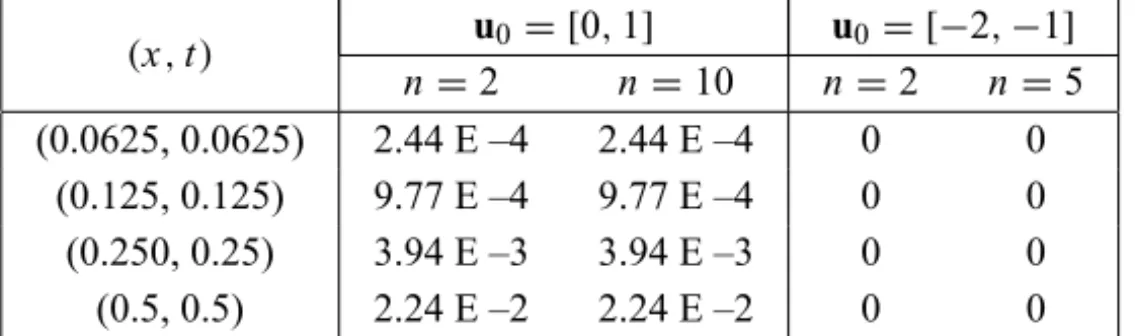
6 Discussion on u0and number of iterations
The problem of choosing initial enclosure u0 seems to be another restrictive difficulty. Table 3 illustrates the piecewise bounds obtained by choosing various initial enclosures and number of iterations:
(x,t) u0= [−2,2] u0= [2,3] u0= [−5,5]
n=2 n=10 n =2 n=5 n=2 n=10
(0.0625, 0.0625) 7.44 E –5 6.19 E –5 0 0 3.23 E –4 6.19 E –5 (0.125, 0.125) 4.55 E –4 2.21 E –4 0 0 5.78 E –3 2.85 E –4 (0.250, 0.25) 3.71 E –3 1.45 E –3 0 0 3.72 E –2 1.45 E –3 (0.5, 0.5) 5.50 E –2 9.47 E –3 0 0 2.41 E 0 5.84 E –1
Table 3 – Diameter of solutions of example 4.1 forpx= pt=16.
Our experimental results in Table 3, show:
(ii) If we choose a proper u0 just a few iteration is needed to achieve rig-orous solutions, moreover increasing the number of iterations can offset inappropriateu0.
Example 2. [14]
u(x,t) = f(x,t)+
Z t
0
Z
G(x,t, ξ, τ )sin(u(ξ, τ ))dξdτ,
(x,t)∈ [0,1] ×,
G(x,t, ξ, τ ) = xt(ξ +τ ),
f(x,t) = −t(x2−sin(x)−xsin(x)),
where= [0,1]andu(x,t)=xt.
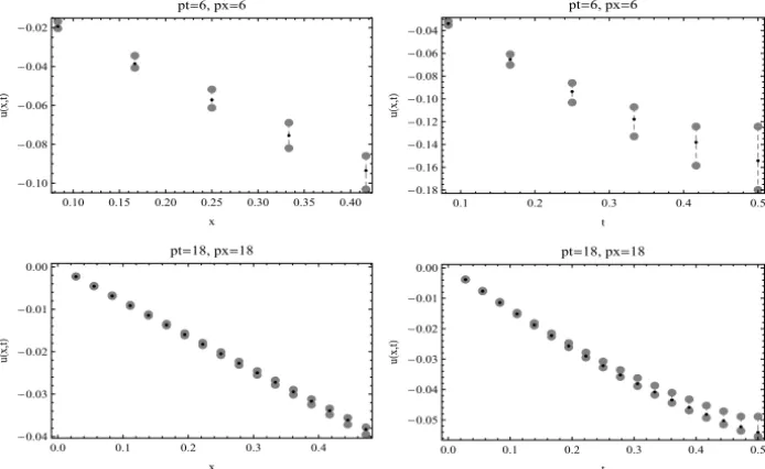
Solution of the equation using the proposed scheme is enclosed in intervals as we show in Table 4 and Figures 3,4. The following experiments are also observed:
(i) Similar to the previous example, for an inaccurate u0 = [−2,−1] the computed interval is empty.
(ii) In many cases, increase the number of iterations does not affect the accu-racy of the results, therefore to increase the accuaccu-racy we need to increase the number of subdivisions (see e.g. Figure 4).
(x,t) u0= [0,1] u0= [−2,−1]
n=2 n =10 n =2 n=5
(0.0625, 0.0625) 2.44 E –4 2.44 E –4 0 0
(0.125, 0.125) 9.77 E –4 9.77 E –4 0 0
(0.250, 0.25) 3.94 E –3 3.94 E –3 0 0
(0.5, 0.5) 2.24 E –2 2.24 E –2 0 0
Table 4 – Diameter of solutions of example 4.2 forpx= pt=16.
7 Conclusion
0.10 0.15 0.20 0.25 0.30 0.35 0.40 0.02 0.04 0.06 0.08 0.10 x u x,t
pt 6, px 6
0.0 0.1 0.2 0.3 0.4 0.00 0.01 0.02 0.03 0.04 x u x,t
pt 18, px 18
0.1 0.2 0.3 0.4 0.5 0.00 0.05 0.10 0.15 0.20 t u x,t
pt 6, px 6
0.0 0.1 0.2 0.3 0.4 0.5 0.00 0.01 0.02 0.03 0.04 0.05 0.06 0.07 t u x,t
pt 18, px 18
Figure 3 – Exact solution of example 4-2 (black dots) is enclosed in piecewise constant
bounds (gray circles).
pt = 3, px = 3 pt = 6, px = 6
0.20 0.25 0.30 0.2 0.3 0.4 0.5 0.00 0.05 0.10 0.15 0.20 0.1 0.2 0.3 0.4 0.1 0.2 0.3 0.4 0.5 0.00 0.05 0.10 0.15 0.20
pt = 9, px = 9 pt = 18, px = 18
0.1 0.2 0.3 0.4 0.1 0.2 0.3 0.4 0.5 0.0 0.1 0.2 0.1 0.2 0.3 0.4 0.1 0.2 0.3 0.4 0.5 0.0 0.1 0.2
paper, we consider an initial enclosure and obtain a new guaranteed bounds for the solution of these equations including all round-off and truncation errors. We also clarify that the algorithm initial enclosures and conditions are not restrictive in practice. Our numerical experiments show that the exact solution is enclosed in intervals where the width of intervals gives the accuracy of the numerical re-sults. This is of great importance, especially when the equations are complicated and the solution is not determined analytically or numerically.
REFERENCES
[1] G. Alefeld and G. Mayer,Interval analysis: theory and applications. J. Comput. Appl. Math.,121(2000), 421–464.
[2] H. Brunner, On the numerical solution of nonlinear Volterra-Fredholm integral equation by collocation methods. SIAM J. Numer. Anal.,27(1990), 987–1000.
[3] H. Brunner and E. Messina,Time-stepping methods for Volterra-Fredholm integral equations by collocation methods. Rend. Math.,23(2004), 329–342.
[4] T.A. Burton,Volterra Integral and Differential Equations. Academic Press, New York (1983).
[5] O. Caprani, K. Madsen and O. Stauning,Enclosing solutions of integral equations. Technical Report, Tech. Univ. of Denmark (1996).
[6] M.B. Dhakne and S.D. Kendre, On abstrct nonlinear mixed Volterra-Fredhom integro-differential equations. Comm. Appl. Nonlinear Anal.,4(2006), 101–112.
[7] O. Diekmann, Thresholds and travelling waves for the geographical spread of infection. J. Math. Biol.,6(1978), 109–130.
[8] H.J. Dobner,Computing narrow inclusions for the solution of integral equations. Numer. Func. Anal. Optim.,10(1989), 923–936.
[9] H.J. Dobner,A method for estimating the solution of integral equations encoun-tered in potential theory. Appl. Math. Comput.,109(2000), 199–204.
[10] K. Domke and L. Hacia,Integral equation in some thermal problem. Int. J. Math. Comput. Simulation,2(2007), 184–189.
[11] W. Edmonson, S. Ocloo, C. Williams and W. Alexander,The use of interval meth-ods in signal processing and control for systems biology edmonson, Foundations of Computational Intelligence, IEEE Symposium (2007), 136–142.
[13] H. Guoqiang,Asymptotic error expansion for the Nystrom method for a nonlinear Volterra-Fredholm equations. J. Comput. Appl. Math.,59(1995).
[14] M. Hadizadeh and Gh. Kazemi, Error estimate in the Sinc collocation method for the Volterra-Fredhlom integral equations based on DE Transformation. Elect. Trans. Numer. Anal.,30(2008), 75–87.
[15] M. Hadizadeh and S. Yazdani,New enclosure algorithms for the verified solutions of nonlinear Volterra integral equations. Appl. Math. Modelling,35(2011), 2972– 2980.
[16] J.P. Kauthen,Continuous time collocation methods for Volterra-Fredholm integral equations. Numer. Math.,56(1989), 409–424.
[17] J.L. Lions,Ariane 5, flight 501 failure. Technical report, European Space Agency (1996).
[18] K. Maleknejad and M. Hadizadeh, A new computational method for Volterra-Fredholm integral equations. Computer Math. Applic.,37(1999), 1–8.
[19] R.E. Moore,Interval Analysis. Prentice-Hall, New York (1966).
[20] R.E. Moore, R.B. Kearfott and M.J. Cloud, Introduction to Interval Analysis. SIAM (2009).
[21] S. Murashige and S. Oishi,Numerical verification of solutions of periodic integral equations with a singular kernel. Numer. Algor.,37(2004), 301–310.
[22] R. Muhanna, H. Zhang and R. Mullen, Interval finite elements as a basis for generalized models of uncertainty in engineering mechanics. Reliab. Comput., 13(2007), 173–194.
[23] M. Neher, K.R. Jackson and N.S. Nedialkov,On Taylor model based integration of ODES.SIAM J. Numer. Anal.,45(2007), 236–262.
[24] H.R. Thieme,A model for the spatial spread of an epidemic,4(1977), 337–351.
[25] H.L. Tidke,Existence of global solutions to nonlinear mixed Volterra-Fredholm integro-differential equations with nonlocal conditions. Electron. J. Diff. Equa.,