Available online at www.ispacs.com/jiasc
Volume 2016, Issue 1, Year 2016 Article ID jiasc-00090, 13 Pages doi:10.5899/2016/jiasc-00090
Research Article
An algorithm for positive solution of boundary value problems
of nonlinear fractional differential equations by Adomian
decomposition method
Hytham. A. Alkresheh1∗, A. I. Md. Ismail1
(1)School of Mathematical Sciences, Universiti Sains Malaysia (USM), 11800, Penang, Malaysia
Copyright 2016 c⃝Hytham. A. Alkresheh and A. I. Md. Ismail. This is an open access article distributed under the Creative Commons Attribution License, which permits unrestricted use, distribution, and reproduction in any medium, provided the original work is properly cited.
Abstract
In this paper, an algorithm based on a new modification, developed by Duan and Rach, for the Adomian decomposition method (ADM) is generalized to find positive solutions for boundary value problems involving nonlinear fractional ordinary differential equations. In the proposed algorithm the boundary conditions are used to convert the nonlinear fractional differential equations to an equivalent integral equation and then a recursion scheme is used to obtain the analytical solution components without the use of undetermined coefficients. Hence, there is no requirement to solve a nonlinear equation or a system of nonlinear equations of undetermined coefficients at each stage of approximation solution as per in the standard ADM. The fractional derivative is described in the Caputo sense. Numerical examples are provided to demonstrate the feasibility of the proposed algorithm.
Keywords:Adomian decomposition method, Fractional boundary value problems, Duan-Rach approach, Caputo derivative.
1 Introduction
Fractional order differential equations (FDEs) have been the subject of considerable interest during the last two decades. It is found to be effective in describing certain applications in the area of engineering, physics [10, 21], fluid-dynamics based traffic models [9], electromagnetism [8], continuum and statistical mechanics [17] and dynam-ics of viscoelastic materials [14]. Several methods have been presented to solve fractional nonlinear BVPs-Adomian decomposition method (ADM) [12], a shifted Legendre spectral method [20], homotopy analysis method [7], gener-alized differential transform method [18], a Chebyshev spectral method [4], Haar wavelet method [23], sinc-Galerkin method [25] and so on .
Some studies have been conducted on the positive solution of fractional nonlinear BVPs. The existence and multiplic-ity results of a positive solution with different types of boundary conditions for fractional differential equations can be found in the works of Xiaojie Xu [29], Sihualiang [15], De-Xiangma [16], Yige Zhao [31], Chengbo Zhai [30], Weihua Jiang [13], Muhammed Syam [26]. Jafary and Daftardar [12] used the standard ADM to find the positive solutions for a fractional nonlinear (Bratu-type) problem involving ordinary differential equations. Jafari and Baghe-rian [11] made a comparison between homotopy perturbation method (HPM) and the standard ADM method.They have shown that the standard ADM method is essentially the HPM method for the fractional nonlinear two point
BVP with 1<α≤2. The standard ADM approach can be improved by utilizing the approach of Duan and Rach [6] for solving BVPs. This approach allows the derivation of a modified recursion scheme for the approximate solution without any undetermined coefficients and avoids the need to solve a nonlinear sequence of algebraic equations for the undetermined coefficients. Dib and Haiahem [3] used the Duan and Rach approach to solve the governing partial differential equation of MHD Jeffery-Hamel flow problem and they showed this approach gives good agreement with the 4th-order Runge-Kutta algorithm and homotopy analysis method.
The purpose of this paper is to generalize the modification proposed by Duan and Rach [6] for the ADM to find a positive solution for the boundary value problems involving nonlinear fractional ordinary differential equations. As will be shown in the next sections, the generalized method is simpler to implement and easy to automate by computer programs. In particular the final solution does not contain any undetermined coefficient at each stage of approximation solution and hence we do not need to use numerical methods to evaluate the values of the undetermined coefficient as in the standard ADM.
There are various definitions of a fractional derivative of orderα (α>0), but the two definitions that are most exten-sively used in applications of fractional calculus are the Riemann-Liouville and Caputo definition [22]. The Caputo fractional derivative which will be used in this study first computes an ordinary derivative followed by a fractional integral to achieve the desired order of fractional derivative while Riemann-Liouville fractional derivative is computed in the reverse order. Hence, the Caputo fractional derivative allows traditional initial and boundary conditions to be included in the formulation of the problem [19].
To provide the setting for this work, we list below some definitions and basic results of others. More details can be found in [22, 24].
Definition 1.1. A real function f(x), x>0,is said to be in the space Cα, α∈Rif there exists a real number p>α, such that f(x) =xpf1(x)is continuous in[0,∞)and it is said to be in the space Cαniff f(n)∈Cα,n∈N0
Definition 1.2. The Riemann-Liouville fractional integral operator of orderα>0, of the function f∈Cµ, µ>−1 is defined as:
Jaαf(t) = 1 Γ(α)
∫ t a(
t−x)α−1f(x)dx, α>0,t>a,a≥0.
1. if α=0, J0αf(t) =f(t)is the identity operator. 2. for f∈Cµ,α,β >0, we have(JaαJ
β
a)(t) = (Jaα+β)(t) 3. if f(t) = (t−a)β for someβ>−1andα>0, then
Jaαf(t) = Γ(β+1)
Γ(n+β+1)(t−a)
n+β.
Definition 1.3. The Caputo fractional derivative of f(t)of orderαwith a>0is defined as:
(Dα∗af)(t) = (Jan−αf(n))(t) = 1 Γ(n−α)
∫ t a
(t−x)n−α−1f
(n)(x)dx,n∈N,n−1<α≤n,
t>a, f(x)∈Cn−1. For this definition we have the following properties:
1. (JaαDα∗af)(t) = f(t)−n∑−1
k=0
(t−a)k
k! f k(a),n
−1<α≤n,n∈N.
2. If f is continuous andα≥0then, DαaJaαf =f .
Dα∗af(t) =
0 ifβ∈ {0,1,2, ...,m−1} Γ(β+1)
Γ(β−n+1)(t−a)
β−α ifβ
∈N0andβ ≥m orβ∈/Nandβ>m−1
2 The proposed method
We first describe modification method of Duan and Rach [6] for the second-order nonlinear ordinary differential equations by using ADM. After that we will generalize this modification for the fractional differential equations case.
Consider the following two-point boundary value problem of the second-order ordinary differential equation
Lu+Nu=f(t), a≤t≤b, (2.1)
u(a) =c1, u(b) =c2, whereL(.) = d2
dt2 is the linear differential operator,Nuis analytic nonlinear term and f(t)known given function.
Take the inverse linear operatorL−1(.)to both sides of Eq.(2.1), whereL−1(.)is defined as
L−1(.) =
∫ t a
∫ t
ζ(.)dtdt, ζ ∈[a,b]is a prescribed value, yields
u(t)−u(a)−u′(ζ)(t−a) =−L−1Nu+L−1f(t). (2.2)
Lett=bin Eq.(2.2). Then solve foru′(ζ), yields
u′(ζ) =u(b)−u(a)
b−a + 1 b−a
([
L−1Nu]t=b−[L−1f(t)]
t=b
)
, (2.3)
where[L−1(.)]
t=b= ∫ b
a ∫ t
ζ(.)dtdt. Substituting Eq.(2.3) in to Eq.(2.2) yields
u(t) =u(a) +u(a)−u(b)
b−a (t−a) +L −1f(t)
−bt−a −a
[
L−1f(t)]
t=b−L−
1Nu+t−a b−a
[
L−1Nu]t=b. (2.4) Thus the approximation solution components by using Duan and Rach modification for the Adomian decomposition method is given by
u0(t) =u(a) +
u(a)−u(b)
b−a (t−a) +L −1f(t)
−bt−a −a
[
L−1f(t)]
t=b (2.5)
un+1(t) =− ∫ t
a ∫ t
ζ (An)dtdt+ t−a b−a
[∫ t a
∫ t
ζ(An)dtdt
]
t=b
, n≥0 (2.6)
whereAnare the Adomian polynomials as will be discussed later in this section.
Now to generalize this modification, we consider the following nonlinear differential equation of fractional order:
subject to the boundary conditionsu(qk)(t
k) =ck, tk∈[a,b], k=0,1,2, ...,m−1. Thetkare not all equal and 0≤q0≤q1≤...≤qm−1such thatqi̸=qjifti=tj.
Also we assume that the positive solution of Eq.(2.7) exists and is unique in the specified interval[a,b].
LetDα∗(.)represent the Caputo fractional derivative of orderα,NuThe analytic nonlinear term, and f(t) is a known given function.
ApplyingL−1(.) =Jα(.)to both sides of Eq.(2.7), whereJαis the Riemann-Liouville fractional integral yields JαDα∗u(t) =Jαf(t)−Jα(Nu).
Using property(1)of definition (1.3)we have
u(t) =
m−1
∑
k=0 Dkf(0)
k! t
k+Jα(f(t))−Jα(Nu) (2.8)
=u(0) +u′(0) +u′′(0)t
2 2 +...+
u(m−1)
(m−1)!t
m−1+Jα(f(t))−Jα(Nu).
The Adomian decomposition method introduces the solution by decomposingu(t)to an infinite seriesu(t) = ∑∞
n=0 un
and the nonlinear termNuby the infinite seriesNu= ∑∞
n=0
AnwhereAnare the Adomian polynomials defined by
An=An(u0,u1, ...,un) = 1 n!
[
dn dλnN
( ∞
∑
n=0
λiu i
)]
λ=0
The polynomialsAnare generated for each nonlinearity so thatA0depends only onu0,A1depends only onu0and u1,A2depends onu0,u1,u2and so on. Many different algorithms to compute the Adomian polynomials have been proposed. See, for example, Adomian and Rach [2], Sheng Duan [5], Wazwaz [28].
The first five Adomian polynomials for the one variableNu=f(u(t))are given by
A0=f(u0), A1=u1f′(u0), A2=u2f′(u0) +
1 2!u
2
1f′′(u0), (2.9)
A3=u3f′(u0) +u1u2f′′(u0) + 1 3!u
3
1f(3)(u0), A4=u4f′(u0) + (u1u3+
1 2!u
2
2)f′′(u0) + 1 2!u
2
1u2f(3)(u0) + 1 4!u
4
1f(4)(u0). There can also can be found from the formula
An= n
∑
ν=1
C(ν,n)f(ν)(u0)
To clarify the method, we take a special case of Eq.(2.7)
Dα∗u(t) +Nu=f(t), 1<α≤2, a≤t≤b,
subject to the boundary conditions, u(a) =c1, u(b) =c2. According to Eq.(2.8) we have
u(t) =u(0) +u′(0)t+L−1(f(t))−L−1(Nu)
=u(0) +u′(0)t+Jα(f(t))−Jα(Nu). (2.10)
Lett=aand thent=bin Eq.(2.10) yields, respectively the two equations
u(a) =u(0) +u′(0)a+ [Jα(f(t))]t=a−[Jα(Nu)]t=a (2.11) u(b) =u(0) +u′(0)b+ [Jα(f(t))]t=b−[Jα(Nu)]t=b. (2.12) Equations (2.11)and(2.12) are two equations with two unknown coefficientsu(0)andu′(0). Solving these two equa-tions with respect to these unknown coefficients yields
u′(0) =u(b)−u(a)
b−a + 1 b−a[J
αf(t)] t=a−
1 b−a[J
αf(t)] t=b−
1 b−a[J
αNu] t=a+
1 b−a[J
αNu]
t=b (2.13)
and
u(0) =u(a)− a
b−a[u(b)−u(a)] + a b−a[J
αf(t)] t=b−
a b−a[J
αf(t)] t=a−
a b−a[J
αNu] t=b+
a b−a[J
αNu] t=a−
[Jαf(t)]t=a+ [JαNu]t=a .
(2.14)
Substituting Eq.(2.13) and Eq.(2.14) in to Eq.(2.10) and simplifying we obtain
u(t) =u(a) +t−a
b−a[u(b)−u(a)] + t−b b−a[J
αf(t)] t=a−
t−a b−a[J
αf(t)] t=b+
b−t b−a[J
αNu] t=a+
t−a b−a[J
αNu] t=b+ Jα(f(t))−Jα(Nu).
(2.15)
Next the nonlinear termNuwill be equated to ∑∞
n=0
AnwhereAnare the Adomian polynomials and decomposing the
solutionu(t)into ∑∞
n=0
un(t). Then applying ADM to Eg.(2.15) yields
u0(t) =u(a) + t−a
b−a[u(b)−u(a)] + t−b b−a[J
αf(t)] t=a−
t−a b−a[J
αf(t)]
t=b+Jα(f(t)), (2.16)
un+1(t) = b−t b−a[J
αA n]t=a+
t−a b−a[J
αA
n]t=b−Jα(An), n≥0. (2.17)
solutions as occurs in the undetermined coefficient method.
Finally thenth-term approximation solution for the Adomian decomposition method is given by
φn= n−1
∑
k=0
uk, n≥1 (2.18)
and the solutionu(t) =lim n→∞φn
3 Illustrative examples
To demonstrate the effectiveness and the simplicity of the proposed method we give two examples with two and three boundary values of nonlinear fractional ordinary differential equation and make a comparison between the results obtained by the proposed method and the exact solution for some values ofα.
3.1 Example [12]
Consider the following Bratu’s type boundary value problem in the form
Dα∗u(t) +eu(t)=0, 1<α≤2, 0≤t≤1, (3.19)
u(0) =0, u(1) =0.
The exact solution of this problem whenα=2 is given in [27] by
u(t) =−2 ln
[
cosh(θt2 −θ4
)
cosh(θ4)
]
, whereθsatisfies the equationθ=√2 cosh(θ4).
To solve this equation by the proposed method, according to the equations (3.16) and (3.17), we obtain
u0(t) =0, (3.20)
(3.21) un+1(t) =t[Jα(An)]t=1−[Jα(An)], n≥0
whereAnare the Adomian polynomials for the nonlinear termNu=euwhich are given by
A0=eu0, (3.22)
A1=u1eu0, A2=
(u2 1 2 +u2
)
eu0,
A3=
(u3 1
6 +u1u2+u3
)
eu0, ...
In view of (3.20), (3.21) and (3.22) we can write the components of the solution for Eq.(3.19) as follows
u0(t) =0, (3.23)
u1(t) = t−tα
αΓ(α),
u2(t) =
4−α(−4αt(−1+tα)Γ(0.5+α) +√π(−t+t2α)Γ(2+α))
In view of (3.23) the approximate solutions of Eq.(3.19) whenn=5 for various value ofα are as follows
Forα=1.2,
φ(t) =0.948641t−0.907604t1.2−0.391384t2.2+0.335435t2.4−0.116044t3.2+0.299552t3.4−
0.166492t3.6−0.0259069t4.2+0.154842t4.4−0.224063t4.6+0.0930731t4.8−
0.00400549t5.2+0.0523022t5.4−0.153367t5.6+0.160541t5.8−0.0555197t6.
(3.24)
Forα=1.6,
φ(t) =0.769751t−0.699484t1.6−0.207002t2.6+0.128921t3.2−0.0439692t3.6+0.0848449t4.2−
0.00697325t4.6−0.0338418t4.8+0.0313441t5.2−0.000694494t5.6−0.0334611t5.8+
0.00686103t6.2+0.010058t6.4−0.0154317t6.8+0.0122721t7.4−0.00319406t8.
(3.25)
Forα=2,
φ(t) =0.549288t−0.5t2−0.0915096t3+0.0291811t4+0.0169618t5−0.00118634t6−
0.00300926t7−0.000272817t8+0.000683422t9−0.000136684t10. (3.26)
The main advantage of using the Duan-Rach modification for solving fractional nonlinear BVP is that evaluating the inverse operator directly at the boundary conditions allows us to find the components of the solution without using numerical methods to calculate the values of the undetermined coefficients as in the standard ADM. For example in the given problem the matching algebraic equations for the approximate solutions by using the standard ADM when
α=2 andn=2,3 are respectively given in [12] by
φ2(t) =βt−
eβt−βt−1
β2
φ3(t) =βt−
eβt−βt−1
β2 −
2βt−eβt(eβt−4βt+4) +5
4β4 .
some of these equations need using numerical methods or some of commands in mathematical programs as the com-mand (Find Root) in mathematica programme to find the values of the undetermined coefficientβ. This cost more time and requires more complicated calculations. Furthermore the accuracy of the approximation solution depend in the accuracy of the values of the undetermined coefficientβ.
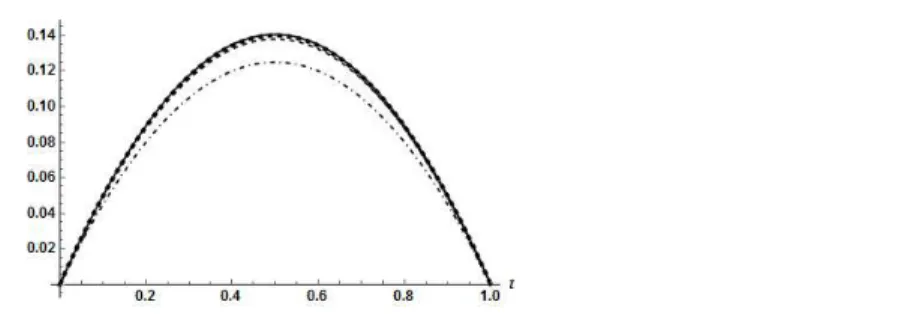
Figure.1 shows the curves of the exact solution and the approximation solutions by the proposed method whenα=2 andn=2,3,4. We note that the curve of the exact solution is in a high agreement with the curve of approximation solution whenn=4 andφn(t)converge to the exact solutionu(t)whenn increases in the interval[0,1]. Figure.2 shows the curves of the approximation solution whenn=6 and various values ofα. Table.1 shows the values of the maximum absolute errorMEn(t)where
Figure 1: uexact(t)(solid line)and the approximation solutionφn(t),φ2(t)(dot-side line),φ3(t)(dashed line),φ4(t) (dot line).
Figure 2:φ6(t),α=1.2 (dot line),α=1.4 (dashed line),α=1.6 (dot-side line),al pha=1.8 (solid line).
Table 1: The maximum absolute error functionMEn(t)forn=3,4,5,6,7 and 0≤t≤1.
n 3 4 5 6 7
|MEn(t)| 2.51838×10⁻³ 4.78451×10⁻⁴ 9.92575×10⁻⁵ 2.17805×10⁻⁵ 4.9696×10⁻⁶
3.2 Example
Consider the three point BVP for inhomogeneous fractional differential equation with(u′)2nonlinearity and 3<α≤4.
Dα∗u(t)−(u′(t))2+g(t) =0, 0≤t≤1, 3<α≤4. (3.27) u(0) =0, u′(0) =0, u′′(0.5) =γ1, u′′′(1) =γ2
whereg(t) = (α+1)2t2α−tΓ(α+2),γ 1=(12)
α−1
α(α+1), γ2=α(α−1)(α+1).
The exact solution for this problemu(t) =tα+1. ApplyingL−1(.) =J(.)to both sides of Eq (3.27) and then us-ing boundary valuesu(0) =0 andu′(0) =0 yields
u(t) =u′′(0)t+u′′′(0)t
2 2 −J
α(g(t)) +Jα((u′(t))2). (3.28)
u′′(0) =γ1− 1 2γ2−
1 2
[
Jα−3(g(t))]
t=1+
[
Jα−2(g(t))]
t=12+
1 2
[
Jα−3(u′(t))2]
t=1−
[
Jα−2(u′(t))2]
t=12. (3.29)
and
u′′′(0) =γ2+[Jα−3(g(t))]t=1−[Jα−3((u′)2)]t=1. (3.30)
Substituting Eq.(3.29) and Eq.(3.30) in to the Eq.(3.28) we obtain
u(t) =t
2
4 (2γ1−γ2) + t3
6γ2+
( t3 6 − t2 4 ) [
Jα−3(g(t))]
t=1+ t2
2
[
Jα−2(g(t))]
t=1 2+ ( t2 4 − t3 6 ) [
Jα−3(u′(t))2]
t=1− t2
2
[
Jα−2((u′(t))2)]
t=1 2−J
α(g(t)) +Jα((u′(t))2).
(3.31)
Applying the ADM in to the Eq.(3.31) we have
u0(t) =t
2
4(2γ1−γ2) + t3
6γ2+
(t3 6 −
t2 4
) [
Jα−3(g(t))]
t=1+ t2
2
[
Jα−2(g(t))]
t=1 2−J
α(g(t)) (3.32)
un+1(t) =
( t2 4 − t3 6 ) [
Jα−3(An)
]
t=1− t2
2
[
Jα−2(An)
]
t=1 2+J
α(A
n), n≥0 (3.33)
whereAnare the Adomian polynomials for the nonlinearity(u′(t))2which given by
An= n
∑
k=0
u′n−ku′k, n≥0 (3.34)
Thus by using the equations (3.32), (3.33)and(3.34) we can calculate the solution components of equation (3.27) when
α=3.9 as follows
u0(t) =−0.851877t2+0.568059t3+t4.9−0.00280675t11.7,
u1(t) =0.754057t2−0.504997t3+0.00971651t5.9−0.00845123t6.9+0.00214008t7.9− 0.00729485t8.8+0.00439289t9.8+0.00280675t11.7+3.68052×10⁻⁶t15.6− 2.81652×10⁻⁶t16.6−5.09743×10⁻⁶t18.5+4.59557×10⁻⁹t25.3,
...
Clearly in this example if we use the standard ADM then we need to solve a system of nonlinear algebraic equations to find the undetermined coefficientsβ1=u′′(0), β2=u′′′(0)at each stage of the approximation solution. Some of these equations may possess non-physical roots. Thus the Duan-Rach modification is an efficient alternative method to the standard ADM for solving BVPs.
Figure 3:uexact(t)(solid line), andφn(t),φ8(t)(dashed line),φ6(t)(dot line),φ4(t)(dot-side line).
Table 2:|MEn(t)|
n 3 4 5 6 7 8
|MEn(t)| 0.0108606 0.00310907 0.0009581 0.000311657 0.000104246 0.0000356986
Figure 4:φ8(t),α=3.2 (dot-dot-side line),α =3.4 (dot-side line),α=3.6 (dot line),α=3.8 (dashed line),α=4 (solid line)
Figure 5:E8(t),α=3.2 (solid line),α=3.4 (dot line),α=3.6 (dot-side line),α =3.8 (dot-dot-side line),α=4 (dashed line)
4 Conclusions
References
[1] G. Adomian, A review of the decomposition method and some recent results for nonlinear equations, Mathe-matical and Computer Modelling, 13 (7) (1990) 17-43.
http://dx.doi.org/10.1016/0895-7177(90)90125-7
[2] G. Adomian, R. Rach, Generalization of Adomian polynomials to functions of several variables, Computers & mathematics with Applications, 24 (5) (1992) 11-24.
http://dx.doi.org/10.1016/0898-1221(92)90037-I
[3] A. Dib, A. Haiahem, B. Bou-Said, An analytical solution of the MHD JefferyHamel flow by the modified Adomian decomposition method, Computers & Fluids, 102 (2014) 111-115.
http://dx.doi.org/10.1016/j.compfluid.2014.06.026
[4] E. Doha, A. Bhrawy, S. Ezz-Eldien, A chebyshev spectral method based on operational matrix for initial and boundary value problems of fractional order, Computers & Mathematics with Applications, 62 (5) (2011) 2364-2373.
http://dx.doi.org/10.1016/j.camwa.2011.07.024
[5] J.-S. Duan, New recurrence algorithms for the nonclassic adomian polynomials, Computers & Mathematics with Applications, 62 (8) (2011) 2961-2977.
http://dx.doi.org/10.1016/j.camwa.2011.07.074
[6] J.-S. Duan, R. Rach, A new modification of the adomian decomposition method for solving boundary value problems for higher order nonlinear differential equations, Applied Mathematics and Computation, 218 (8) (2011) 4090-4118.
http://dx.doi.org/10.1016/j.amc.2011.09.037
[7] A. El-Ajou, O. A. Arqub, S. Momani, Solving fractional two-point boundary value problems using continuous analytic method, Ain Shams Engineering Journal, 4 (3) (2013) 539-547.
http://dx.doi.org/10.1016/j.asej.2012.11.010
[8] N. Engheta, On fractional calculus and fractional multipoles in electromagnetism, Antennas and Propagation, IEEE Transactions on, 44 (4) (1996) 554-566.
http://dx.doi.org/10.1109/8.489308
[9] J. He, Some applications of nonlinear fractional differential equations and their approximations, Bull. Sci. Tech-nol, 15 (2) (1999) 86-90.
[10] J. He, Nonlinear oscillation with fractional derivative and its applications, in: International conference on vibrat-ing engineervibrat-ing, 98 (1998) 288-291.
[11] H. Jafari, K. Bagherian, S. P. Moshokoa, Homotopy perturbation method to obtain positive solutions of nonlinear boundary value problems of fractional order, in: Abstract and Applied Analysis, Vol. 2014, Hindawi Publishing Corporation, 2014.
http://dx.doi.org/10.1155/2014/919052
[12] H. Jafari, V. Daftardar-Gejji, Positive solutions of nonlinear fractional boundary value problems using adomian decomposition method, Applied Mathematics and Computation, 180 (2) (2006) 700-706.
http://dx.doi.org/10.1016/j.amc.2006.01.007
[13] W. Jiang, B. Wang, Z. Wang, The existence of positive solutions for multipoint boundary value problems of fractional differential equations, Physics Procedia, 25 (2012) 958-964.
[14] C. Lederman, J.-M. Roquejoffre, N. Wolanski, Mathematical justification of a nonlinear integro-differential equation for the propagation of spherical ames, Annali di Matematica Pura ed Applicata, 183 (2) (2004) 173-239.
http://dx.doi.org/10.1007/s10231-003-0085-1
[15] S. Liang, J. Zhang, Positive solutions for boundary value problems of nonlinear fractional differential equation, Nonlinear Analysis: Theory, Methods & Applications, 71 (11) (2009) 5545-5550.
http://dx.doi.org/10.1016/j.na.2009.04.045
[16] De-xiang Ma, Positive solutions of multi-point boundary value problem of fractional differential equation, Arab Journal of Mathematical Sciences, 21 (2) (2015) 225236.
http://dx.doi.org/10.1016/j.ajmsc.2014.11.001
[17] F. Mainardi, Fractional calculus: some basic problems in countinuum and statistical mechanics, Fractals and Fractional Calculus in Continuum Mechanics, 378 (1997) 291-348.
[18] A. D. Matteo, A. Pirrotta, Generalized differential transform method for nonlinear boundary value problem of fractional order, Communications in Nonlinear Science and Numerical Simulation, 29 (13) (2015) 88101. http://dx.doi.org/10.1016/j.cnsns.2015.04.017
[19] S. Momani, N. Shawagfeh, Decomposition method for solving fractional riccati differential equations, Applied Mathematics and Computation, 182 (2) (2006) 1083-1092.
http://dx.doi.org/10.1016/j.amc.2006.05.008
[20] A. H. Bhrawy, M. M. Al-Shomrani, A shifted legendre spectral method for fractional-order multi-point boundary value problems, Advances in Difference Equations, 2012 (1) (2012) 1-19.
http://dx.doi.org/10.1186/1687-1847-2012-8
[21] I. Podlubny, Geometric and physical interpretation of fractional integration and fractional differentiation, arXiv preprint math/0110241, 5 (4) (2002) 367-386.
[22] I. Podlubny, Fractional differential equations: an introduction to fractional derivatives, fractional differential equations, to methods of their solution and some of their applications, Vol. 198, Academic press, 1998.
[23] U. Saeed, M. ur Rejman, M. A. Iqbal, Haar wavelet-picard technique for fractional order nonlinear initial and boundary value problems, Scientific Research and Essays, 9 (12) (2014) 571-580.
http://dx.doi.org/10.5897/SRE2013.5777
[24] S. G. Samko, A. A. Kilbas, O. I. Marichev, Fractional integrals and derivatives: Theory and applications, 1993, Gordon and Breach, Yverdon.
[25] A. Secer, S. Alkan, M. A. Akinlar, M. Bayram, Sinc-galerkin method for approximate solutions of fractional order boundary value problems, Boundary Value Problems, 2013 (1) (2013) 1-14.
http://dx.doi.org/10.1186/1687-2770-2013-281
[26] M. Syam, M. Al-Refai, Positive solutions and monotone iterative sequences for a class of higher order boundary value problems of fractional order, Journal of Fractional Calculus and Applications, 4 (1) (2013) 147-159.
[27] A.-M. Wazwaz, Adomian decomposition method for a reliable treatment of the bratu-type equations, Applied Mathematics and Computation, 166 (3) (2005) 652-663.
http://dx.doi.org/10.1016/j.amc.2004.06.059
[28] A.-M. Wazwaz, A new algorithm for calculating adomian polynomials for nonlinear operators, Applied Mathe-matics and computation, 111 (1) (2000) 33-51.
[29] X. Xu, D. Jiang, C. Yuan, Multiple positive solutions for the boundary value problem of a nonlinear fractional differential equation, Nonlinear Analysis: Theory, Methods & Applications, 71 (10) (2009) 4676-4688. http://dx.doi.org/10.1016/j.na.2009.03.030
[30] C. Zhai, L. Xu, Properties of positive solutions to a class of four-point boundary value problem of caputo frac-tional differential equations with a parameter, Communications in Nonlinear Science and Numerical Simulation, 19 (8) (2014) 2820-2827.
http://dx.doi.org/10.1016/j.cnsns.2014.01.003
[31] Y. Zhao, S. Sun, Z. Han, Q. Li, The existence of multiple positive solutions for boundary value problems of nonlinear fractional differential equations, Communications in Nonlinear Science and Numerical Simulation, 16 (4) (2011) 2086-2097.