ISSN 1549-3636
© 2009 Science Publications
864
Optimizing Feature Construction Process for Dynamic Aggregation
of Relational Attributes
Rayner Alfred
School of Engineering and Information Technology,
University Malaysia Sabah, Locked Bag 2073, 88999, Kota Kinabalu, Sabah, Malaysia
Abstract: Problem statement: The importance of input representation has been recognized already in machine learning. Feature construction is one of the methods used to generate relevant features for learning data. This study addressed the question whether or not the descriptive accuracy of the DARA algorithm benefits from the feature construction process. In other words, this paper discusses the application of genetic algorithm to optimize the feature construction process to generate input data for the data summarization method called Dynamic Aggregation of Relational Attributes (DARA). Approach: The DARA algorithm was designed to summarize data stored in the non-target tables by clustering them into groups, where multiple records stored in non-target tables correspond to a single record stored in a target table. Here, feature construction methods are applied in order to improve the descriptive accuracy of the DARA algorithm. Since, the study addressed the question whether or not the descriptive accuracy of the DARA algorithm benefits from the feature construction process, the involved task includes solving the problem of constructing a relevant set of features for the DARA algorithm by using a genetic-based algorithm. Results: It is shown in the experimental results that the quality of summarized data is directly influenced by the methods used to create patterns that represent records in the (n×p) TF-IDF weighted frequency matrix. The results of the evaluation of the genetic-based feature construction algorithm showed that the data summarization results can be improved by constructing features by using the Cluster Entropy (CE) genetic-based feature construction algorithm. Conclusion: This study showed that the data summarization results can be improved by constructing features by using the cluster entropy genetic-based feature construction algorithm.
Key words: Feature construction, feature transformation, data summarization, genetic algorithm, clustering
INTRODUCTION
Learning is an important aspect of research in Artificial Intelligence (AI). Many of the existing learning approaches consider the learning algorithm as a passive process that makes use of the information presented to it. This paper studies the application of feature construction to improve the descriptive accuracy of a data summarization algorithm, which is called Dynamic Aggregation of Relational Attributes (DARA)[1]. The DARA algorithm summarizes data stored in non-target tables that have many-to-one relationships with data stored in the target table. As one of the feature transformation methods, feature construction methods are mostly related to classification problems where the data are stored in target table. In this case, the predictive accuracy can often be significantly improved by constructing new features which are more relevant for predicting the class of an object. On the other hand, feature construction
also has been used in descriptive induction algorithms, particularly those algorithms that are based on inductive logic programming (e.g., Warmr[2] and Relational Subgroup Discovery (RSD)[3]), in order to discover patterns described in the form of individual rules.
865 table, in the TF-IDF[4] weighted frequency matrix in order to cluster these objects.
Dynamic Aggregation of Relational Attributes (DARA): The DARA algorithm is designed to summarize relational data stored in the non-target tables. The data summarization method employs the TF-IDF weighted frequency matrix (vector space model[4]) to represent the relational data model, where the representation of data stored in multiple tables will be analyzed and it will be transformed into data representation in a vector space model. The term data summarization is commonly used to summarize data stored in relational databases with one-to-many relations[5,6]. Here, we define the term data summarization in the context of summarizing data stored in non-target tables that correspond to the data stored in the target table. We first define the terms target and non-target tables.
Definition 1: Target table, T, is a table that consists of rows of object where each row represents a single unique object and this is the table in which patterns are extracted.
Definition 2: A non-target table, NT, is a table that consists of rows of objects where a subset of these rows can be linked to a single object stored in the target table.
Based on the definitions defined in 1 and 2, the term data summarization can be defined as follows: Definition 3: Data summarization for data stored in multiple tables with one-to-many relations can be defined as follows:
• A target table T
• Records in the target table RT
• A non-target table NT
• Records in non-target table RNT
Where, one or more RNT can be linked to a single
RT, a data summarization for all RNT in NT is defined as
a process of appending to T at least one field characterizing the values of RNT linked to each RT in T.
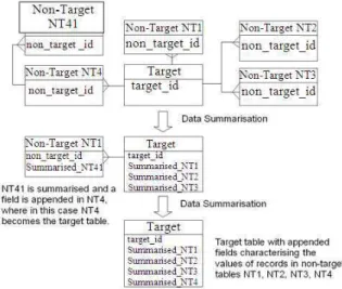
Figure 1 shows the process of data summarization for a target table T that has one-to-many relationships with all non-target tables (NT1, NT2, NT3, NT4, NT41). Since NT4 has a one-to-many relationship with NT41, NT4 becomes the target table in order to summarize the non-target table NT41.
Fig. 1: Data summarization for data stored in multiple tables with one-to-many relations
The summarised_NT1, summarised_NT2, summarised_NT3 and summarised_NT4 fields characterize the values of RNT linked to T, and these
fields are appended to the list of existing attributes in target table T.
In order to classify records stored in the target table that have one-to-many relations with records stored in non-target tables, the DARA algorithm transforms the representation of data stored in the non-target tables into an (n×p) matrix in order to cluster these records (Fig. 2), where n is the number of records to be clustered and p is the number of patterns considered for clustering. As a result, the records stored in the non-target tables are summarized by clustering them into groups that share similar characteristics. Clustering is considered as one of the descriptive tasks that seeks to identify natural groupings in the data based on the patterns given. Developing techniques to automatically discover such groupings is an important part of knowledge discovery and data mining research.
866
Fig. 2: Feature transformation process for data stored in multiple tables with one-to-many relations into a vector space data representation
For instance, given a non-target table with attributes (Fa, Fb, Fc), all possible constructed features are Fa, Fb,
Fc, FaFb, FbFc, FaFc and FaFbFc. These newly constructed
features will be used to produce patterns or instances to represent records stored in the non-target table, in the (n×p) TF-IDF weighted frequency matrix. After the records stored in the non-target relation are clustered, a new column, Fnew, is added to the set of original
features in the target table. This new column contains the cluster identification number for all records stored in the non-target table. In this way, we aim to map data stored in the non-target table to the records stored in the target table.
MATERIALS AND METHODS
Here, we explain the process of feature transformation, particularly feature construction and discuss some of the feature scoring methods used to evaluate the quality of the newly constructed features. Feature transformation in machine learning: In order to generate patterns for the purpose of summarizing data stored in the non-target tables, there are several benefits of applying feature transformation to generate new features that include:
• The improvement of the descriptive accuracy of the data summarization by generating relevant patterns describing each object stored in the non-target table • Facilitating the predictive modelling task for the data stored in the target table, when the summarized data are appended to the target table (e.g., the newly constructed feature, Fnew, is added
to the set of original features given in the target table as shown in Fig. 2)
• Optimizing the feature space to describe objects stored in the non-target table
The input representation for any learning algorithm can be transformed to improve accuracy for a particular task. Feature transformation can be defined as follows: Definition 4: Given a set of features Fs and the training set T, generate a representation Fc derived from Fs that
maximizes some criterion and is at least as good as Fs with respect to that criterion.
The approaches that follow this scheme can be categorized into three categories:
867 Feature weighting: The problem of feature weighting can be defined as the task of assigning weights to the features that describe the hypothesis at least as well as the original set without any weights. The weight reflects the relative importance of a feature and may be utilized in the process of inductive learning. This feature weighting method is mostly beneficial for the distance-based classifier[7].
Feature construction: The problem of feature construction can be defined as the task of constructing new features, based on some functional expressions that use the values of original features that describe the hypothesis at least as well as the original set.
In this study, we apply the feature construction methods to improve the descriptive accuracy of the DARA algorithm.
Feature construction: Feature construction consists of constructing new features by applying some operations or functions to the original features, so that the new features make the learning task easier for a data mining algorithm[8,9]. This is achieved by constructing new features from the given feature set to abstract the interaction among several attributes into a new one. For instance, a simple example of this is when given a set of features {F1, F2, F3, F4, F5}, one could have (F1∧ F2),
(F3 ∧ F4), (F5∧ F1) as the possible constructed features.
In this work, we focus on this most general and promising approach in constructing features to summarize data in a multi-relational setting.
With respect to the construction strategy, feature construction methods can be roughly divided into two groups: Hypothesis-driven methods and data-driven methods[10]. Hypothesis-driven methods construct new features based on the previously-generated hypothesis (discovered rules). They start by constructing a new hypothesis and this new hypothesis is examined to construct new features. These new features are then added to the set of original features to construct another new hypothesis again. This process is repeated until the stopping condition is satisfied. This type of feature construction is highly dependent on the quality of the previously generated hypotheses. On the other hand, data-driven methods, such as GALA[11] and GPCI[12], construct new features by directly detecting relationships in the data. GALA constructs new features based on the combination of booleanised original features using the two logical operators, AND and OR. GPCI is inspired by GALA, in which GPCI used an evolutionary algorithm to construct features. One of the disadvantages of GALA and GPCI is that the booleanization of features can lead to a significant loss of relevant information[13].
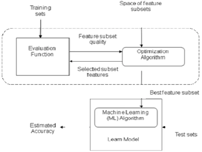
Fig. 3: Illustration of the Filter approach to feature subset selection
Fig. 4: Illustration of the Wrapper approach to feature subset selection
There are essentially two approaches to constructing features in relation to data mining. The first method is as a separate, independent pre-processing stage, in which the new attributes are constructed before the classification algorithm is applied to build the model[14]. In other words, the quality of a candidate new feature is evaluated by directly accessing the data, without running any inductive learning algorithm. In this approach, the features constructed can be fed to different kinds of inductive learning methods. This method is also known as a Filter approach, which is showed in Fig. 3.
868 feature is evaluated by executing the inductive learning algorithm used to extract knowledge from the data, so that in principle the constructed features’ usefulness tends to be limited to that inductive learning algorithm. In this study, the filtering approach that uses the data-driven strategy is applied to construct features for the descriptive task, since the wrapper approaches are computationally more expensive than the filtering approaches.
Feature scoring: The scoring of the constructed feature can be performed using some of the measures used in machine learning, such as information gain (Eq. 1) and cross entropy (Eq. 6), to assign a score to the constructed feature. For instance, the ID3 decision-tree[17] induction algorithm applies information gain to evaluate features. The information gain of a new feature F, denoted InfoGain(F), represents the difference of the class entropy in data set before the usage of feature F, denoted Ent(C), and after the usage of feature F for splitting the data set into subsets, denoted Ent(C|F), as shown in Eq. 1:
infoGain (F) = Ent(C)-Ent(C|F) (1) Where:
( )
nj 1
2
j j
Ent C Pr(C ).log Pr (C )
=
= −
∑
(2)and
(
)
n n
j 1 j 1
2
i j i j i
Ent(C | F) Pr (F ).( Pr(C | F ).log Pr C | F )
= =
=−
∑
∑
− (3)where, Pr(Cj) is the estimated probability of observing
the jth class, n is the number of classes, Pr(Fi) is the
estimated probability of observing the ith value of feature F, m is the number of values of the feature F, and Pr(Cj |Fi) is the probability of observing the jth
class conditional on having observed the ith value of the feature F. Information Gain Ratio (IGR) is sometimes used when considering attributes with a large number of distinct values. The Information Gain Ratio of a feature, denoted by IGR(F), is computed by dividing the Information Gain, InfoGain(F) shown in Equation 1, by the amount of information of the feature F, denoted Ent(F):
InfoGain (F) IGR (F) Ent(F) = (4) Where: m
i 2 i
i 1
Ent(F) Pr (F ).log Pr(F )
=
=−∑ (5)
and Pr(Fi) is the estimated probability of observing the
ith value of the feature F and m is the number of values of the feature F.
Another feature scoring used in machine learning is cross entropy[18]. Koller and Sahami[18] define the task of feature selection as the task of finding a feature subset Fs such that
i
s
Pr(C | F )is close to
i
o
Pr(C | F ), where C is a set of classes,
i
s
Pr(C | F )are the estimated probabilities of observing the ith value of the feature Fs that belongs to class C and
i
o
Pr(C | F ) are the estimated probabilities of observing the ith value of the feature Fo
that belongs to class C. The extent of error if one distribution is substituted by the other is called the cross entropy between two distributions. Let α be the distribution of the original feature set and β be the approximated distribution due the reduced feature set. Then the cross entropy can be expressed as:
x
(x) CrossEnt( , ) (x) log
(x)
εα
α
α β = α
β
∑
(6)in which a feature set Fs that minimizes:
k i i 1
s i
Pr (F ).CrossEnt (Pr(C | F ), Pr(C | F ))
=
∑
(7)is the optimal subset, where k is the number of features in the dataset. Next, we will describes the process of feature construction for data summarization and introduces a genetic-based (i.e., evolutionary) feature construction algorithm that uses a non-algebraic form to represent an individual solution to construct features. This genetic-based feature construction algorithm constructs features to produce patterns that characterize each unique object stored in the non-target table. Feature construction for data summarization: In the DARA algorithm[1], the patterns produced to represent objects in the TF-IDF weighted frequency matrix are based on simple algorithms. These patterns are produced based on the number of attributes combined that can be categorized into three categories. These categories include:
869 Fig. 5: Illustration of the Filtering approach to feature
construction
• a set of patterns produced from the combination of all attributes by using the PAll algorithm
• a set of patterns produced from variable length attributes that are selected and combined randomly from the given attributes
For example, given a set of attributes {F1, F2, F3,
F4, F5}, one could have (F1, F2, F3, F4, F5) as the
constructed features by using the PSingle algorithm. In
contrast, with the same example, one will only have a single feature (F1F2F3F4F5) produced by using the PAll
algorithm. As a result, data stored across multiple tables with high cardinality attributes can be represented as bags of patterns produced using these constructed features. An object can also be represented by patterns produced on the basis of randomly constructed features (e.g., (F1F5, F2F4, F3)), where features are combined
based on some pre-computed feature scoring measures. This work studies a filtering approach to feature construction for the purpose of data summarization using the DARA algorithm (Fig. 5). A set of constructed features is used to produce patterns for each unique record stored in the non-target table. As a result, these patterns can be used to represent objects stored in the non-target table in the form of a vector space. The vectors of patterns are then used to construct the TF-IDF weighted frequency matrix. Then, the clustering technique can be applied to categories these objects. Next, the quality of each set of the constructed features is measured. This process is repeated for the other sets of constructed features. The set of constructed features
that produces the highest measure of quality is maintained to produce the final clustering result. Genetic-based approach to feature construction for data summarization: Feature construction methods that are based on greedy search usually suffer from the local optima problem. When the constructed feature is complex due to the interaction among attributes, the search space for constructing new features has more variation. An exhaustive search may be feasible, if the number of attributes is not too large. In general, the problem is known to be NP-hard[19] and the search becomes quickly computationally intractable. As a result, the feature construction method requires a heuristic search strategy such as Genetic Algorithms to be able to avoid the local optima and find the global optima solutions[20,21]. Genetic Algorithms (GA) are a kind of multidirectional parallel search, and viable alternative to the intractable exhaustive search and complicated search space[22, 23]. For this reason, we also use a GA-based algorithm to construct features for the data summarization task. We will describe a GA-based feature construction algorithm that generates patterns for the purpose of summarizing data stored in the non-target tables. With the summarized data obtained from the related data stored in the non-target tables, the DARA algorithm may facilitate the classification task performed on the data stored in the target table.
Individual representation: There are two alternative representations of features: algebraic and non-algebraic[21]. In algebraic form, the features are shown by means of some algebraic operators such as arithmetic or Boolean operators. Most genetic-based feature construction methods like GCI[14], GPCI[12] and Gabret[24] apply the algebraic form of representation using a parse tree[25]. GPCI uses a fix set of operators, AND and NOT, applicable to all Boolean domains. The use of operators makes the method applicable to a wider range of problems. In contrast, GCI[14] and Gabret[24] apply domain-specific operators to reduce complexity. In addition to the issue of defining operators, an algebraic form of representation can produce an unlimited search space since any feature can appear in infinitely many forms[21]. Therefore, a feature construction method based on an algebraic form needs a restriction to limit the growth of constructed functions.
Features can also be represented in a non-algebraic form, in which the representation uses no operators. For example, in this work, given a set of attributes {X1,X2,X3,X4,X5}, a feature in an algebraic form like
870 non-algebraic form as <X1X2X3X4X5, 2>, where the
digit, “2”, refers to the number of attributes combined to generate the first constructed feature.
The non-algebraic representation of features has several advantages over the algebraic representation[21]. These include the simplicity of the non-algebraic form to represent each individual in the process of constructing features, since there are no operators required. Next, when using a genetic-based algorithm to find the best set of features constructed, traversal of the search space of a non-algebraic is much easier. For example, given a set of features, a parameter expressing the number of attributes to be combined and the point of reordering, one may have the following set of features in a non-algebraic form, <X1X2X3X4X5, 3, 2>.
The first digit, “3”, refers to the number of attributes combined to construct the first feature, where the attributes are unordered, and the second digit, “2”, refers to the index of the column where the order of the features in the set is reordered during the reordering process. The second feature is constructed by combining the attributes remaining in the set. For instance, if the first constructed feature is (X2X4X5)
from a given set of attributes (X1X2X3X4X5), the second
constructed feature is (X1X3). After the reordering
process, a new set of features in a non-algebraic form can be represented as <X3X4X5X1X2, 3, 2>.
Table 1 shows the algorithm to generate a series of constructed features. Given F as a set of l attributes and the number of attributes to be combined, n, where 1≤n≤l, the algorithm starts by randomly selecting n number of attributes. The n selected attributes are then combined to form a new feature, FNi and added into the
set of constructed features, FC. These selected attributes
are then removed from the original set of attributes, F. The process of constructing new features is repeated until the numbers of attributes left in F is less than the total number of attributes combined, n. The remaining attributes left in F are then combined to form the last feature and then this new constructed feature is added to FC. Table 2 shows the sequence of constructing
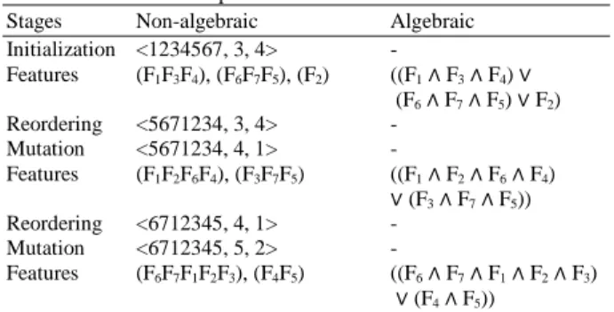
features using the genetic-based algorithm starting from the population initialization and also illustrates the representation of the constructed features in the algebraic and non-algebraic forms. During the population initialization, each chromosome is initialized with the following format, <X, A, B>, where:
• X represents a list of the attribute’s indices • A represents the number of attributes combined
• B represents the point of reordering the sequence of attribute’s indices
Thus, given a chromosome <1234567, 3, 4>, where the list 1234567 represents the sequence of seven attributes, the digit “3” represents the number of attributes combined and the digit “4” represents the point of reordering the sequence of attribute’s indices, the possible constructed features are (F1F3F4), (F6F7F5)
and (F2), with the assumption that the attributes are
selected randomly from attribute F1 through attribute F7
to form the new features. The reordering process simply copies the sequence (string of attributes), (1234567), and rearranges it so that its tail, (567), is moved to the front to form the new sequence (5671234). The mutation process simply changes the number of attributes combined, A, and the point of reordering in the string, B. The rest of the feature representations can be obtained by mutating A, and B, and these values should be less than or equal to the number of attributes considered in the problem. As a result, this form of representation results in more variation after performing genetic operators and can provide more useful features.
Table 1: The algorithm to generate a series of constructed features
Algorithm: Generating list of constructed features
INPUT: A set of original features F = (F1, F2, F3,...,Fl), n number of attributes
Output: A set of constructed features FC 01) Initialize counter i = 1
02) Pick n attributes randomly and construct a new feature, FNi 03) Add FNi to FC, FC∪ FNi, and increment i
04) l′ = l − n. 05) IF l′ > n THEN 06) l = l′
07) GOTO 02 08) ELSE
09) Construct a new feature based on the remaining attributes, FNi 10) Add FNi to FC, FC∪ FNi, STOP
11) END
Table 2: Features in the non-algebraic and algebraic forms: Population Initialization, Features construction, Reordering and Mutation processes
Stages Non-algebraic Algebraic Initialization <1234567, 3, 4> -
Features (F1F3F4), (F6F7F5), (F2) ((F1∧ F3∧ F4) ∨ (F6∧ F7∧ F5) ∨ F2) Reordering <5671234, 3, 4> -
Mutation <5671234, 4, 1> -
Features (F1F2F6F4), (F3F7F5) ((F1∧ F2∧ F6∧ F4)
∨ (F3∧ F7∧ F5)) Reordering <6712345, 4, 1> -
Mutation <6712345, 5, 2> -
Features (F6F7F1F2F3), (F4F5) ((F6∧ F7∧ F1∧ F2∧ F3)
871 Fitness functions: Information Gain (Eq. 1) is often used as a fitness function to evaluate the quality of the constructed features in order to improve the predictive accuracy of a supervised learner[26,13]. In contrast, if the objective of the feature construction is to improve the descriptive accuracy of an unsupervised clustering technique, one may use the Davies-Bouldin Index (DBI)[27] as the fitness function. However, if the objective of the feature construction is to improve the descriptive accuracy of a semi-supervised clustering technique, the total cluster entropy (Eq. 8) can be used as the fitness function to evaluate how well the newly constructed feature clusters the objects.
In our approach to summarizing data in a multi-relational database, in order to improve the predictive accuracy of a classification task, the fitness function for the GA-based feature construction algorithm can be defined in several ways. In these experiments, we examine the case of semi-supervised learning to improve the predictive accuracy of a classification task. As a result, we will perform experiments that evaluate four types of feature-scoring measures (fitness functions) outlined below:
• Information Gain (Eq. 1) • Total Cluster Entropy (Eq. 8)
• Information Gain coupled with Cluster Entropy (Eq. 11)
• Davies-Bouldin Index[27]
The information gain (Eq. 1) of a feature F represents the difference of the class entropy in data set before the usage of feature F and after the usage of feature F for splitting the data set into subsets. This information gain measure is generally used for classification tasks. On the other hand, if the objective of the data modeling task is to separate objects from different classes (like different protein families, types of wood, or species of dogs), the cluster’s diversity, for the kth cluster, refers to the number of classes within the kth cluster. If this value is large for any cluster, there are many classes within this cluster and there is a large diversity. In this genetic approach to feature construction for the proposed data summarization technique, the fitness function can also be defined as the diversity of the clusters produced. In other words, the fitness of each individual non-algebraic form of constructed features depends on the diversity of each cluster produced.
In these experiments, in order to cluster a given set of categorized records into K clusters, the fitness
function for a given set of constructed features is defined as the total clusters entropy, H(K), of all clusters produced (Eq. 8). This is also known as the Shannon-Weiner diversity[28,29]:
N k k K 1n .H H(K)
N
=
=
∑
(8)Where:
nk = The number of objects in kth cluster
N = The total number of objects
Hk = The entropy of the kth cluster, which is defined
in Eq. 9 Where:
S = The number of classes Psk = The probability that an
object randomly chosen from the kth cluster belongs to the sth class
S
s 1
2
k sk. sk
H P log (P )
=
=−∑ (9)
The smaller the value of the fitness function using the total Cluster Entropy (CE), the better is the quality of clusters produced. Another metric that can be used to evaluate the goodness of the clustering result is called the purity of the cluster or this metric is better known as the measure of dominance, MDk, shown in Eq. 10,
which is developed by Berger and Parker[30]:
( )
sk kk
MAX n MD
n
= (10)
Where:
MAX(nsk) = Just the number of objects in the most
abundant class, s, in cluster k nk = The number of objects in cluster k
Next, we will also study the effect of combining the Information Gain (Eq. 1) and Total Cluster Entropy (Eq. 8) measures, denoted as CE_IG(F,K), as the fitness function in our genetic algorithm, as shown in equation 11, where K is the number of clusters and F is the constructed feature:
CE_IG (F,K) = InfoGain(F) + 1 N
k k k n H.
N
=
∑
872 Finally, these experiments also evaluate the effectiveness of the feature construction methods based on the quality of the cluster’s structure. The effectiveness is measured using the Davies-Bouldin Index (DBI)[27], to improve the predictive accuracy of a classification task.
RESULTS AND DISCUSSION
In these experiments we observe the influence of the constructed features for the DARA algorithm on the final result of the classification task. Referring to Fig. 2, the constructed features are used to generate patterns representing the characteristics of records stored in the non-target tables. These characteristics are then summarised and the results appended as a new attribute into the target table. The classification task is then carried out as before. The Mutagenesis databases (B1, B2, B3)[31] and Hepatitis databases (H1, H2, H3) from PKDD 2005 are chosen for these experiments.
The genetic-based feature construction algorithm used in these experiments applies different types of fitness functions to construct the set of new features. These fitness functions include the Information Gain (IG) (Eq. 1), Total Cluster Entropy (CE) (Eq. 8), the combined measures of Information Gain and Total Cluster Entropy (CE-IG) (Eq. 11) and, finally, the Davies-Bouldin Index (DBI)[27]. For each experiment, the evaluation is repeated ten times independently with ten different numbers of clusters, k, 10 ranging from 3-21. The J48 classifier (as implemented in WEKA[32]) is used to evaluate the quality of the constructed features based on the predictive accuracy of the classification task. Hence, in these experiments we compare the predictive accuracy of the decision trees produced by the J48 for the data when using PSingle and PAll methods.
The performance accuracy is computed using the 10-fold cross-validation procedure.
In addition to the goal of evaluating the quality of the constructed features produced by the genetic-based algorithm, our experiments also have the goal of determining how robust the genetic-based feature construction approach is to variations in the setting of the number of clusters, k, where k = 3, 5,7,9,11, 13,15,17,19,21. Other parameters include reordering probability, pc = 0.80, mutation probability, pm = 0.50,
population size is set to 500 and the number of generations is set to 100. In these experiments, we made no attempt to optimize the parameters mentioned in this study. The results for the mutagenesis (B1, B2, B3) and hepatitis (H1, H2, H3) datasets are reported in Table 3. Table 3 shows the average performance accuracy of the
J48 classifier (for all values of k), using a 10-fold cross-validation procedure. The predictive accuracy results of the J48 classifier are higher when the genetic-based feature construction algorithms are used compared to the predictive accuracy results for the data with features constructed using the PSingle and PAll methods.
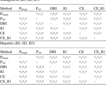
Table 4 shows the results of paired t-test (p = 0.05) for mutagenesis and hepatitis datasets. In this table, the symbol ’⊕’ indicates significant improvement in performance by method in row over method in column and the symbol ’⊖’ indicates no significant improvement in performance by method in row over method in column, on the three datasets. For the Mutagenesis datasets, there is a significant improvement in predictive accuracy for the CE genetic-based feature construction method over the other genetic-based feature construction methods including IG, CE_IG and DBI methods, and the feature construction methods using the PSingle and PAll algorithms. In addition to that, significant
improvements in predictive accuracy for the J48 classifier are recorded for the genetic-based feature construction methods with fitness functions DBI, GI, CE_IG and CE over the feature construction methods using the PSingle and PAll algorithms, for the hepatitis
datasets.
Table 3: Predictive accuracy results based on 10-fold cross-validation using J48 (C4.5) classifier (mean ± SD)
PSingle PAll CE CE_IG IG DBI
B1 80.9±1.4 80.0±2.0 81.8±1.3 81.3±0.7 81.3±0.7 78.6±2.9 B2 81.1±1.4 79.2±3.0 82.4±1.5 80.3±2.1 80.2±2.3 78.8±1.3 B3 78.8±3.3 79.2±5.7 85.3±3.9 84.4±3.9 75.5±4.7 78.9±4.6 H1 70.3±1.6 72.3±1.7 75.1±2.5 75.2±2.4 74.9±2.5 74.0±2.0 H2 71.8±2.9 74.7±1.3 77.1±3.3 76.9±3.0 76.3±3.8 76.1±2.1 H3 72.3±3.0 74.8±1.3 77.1±3.3 76.4±3.8 76.5±3.9 76.3±2.6
Table 4: Results of paired t-test (p = 0.05) for mutagenesis and hepatitis PKDD 2005 datasets
Mutagenesis (B1, B2, B3)
---
Method PSingle PAll DBI IG CE CE_IG
PSingle - , , , , , , , , , ,
PAll , , - , , , , , , , ,
DBI , , , , - , , , , , ,
IG , , , , , , - , , , ,
CE , , , , , , , , - , ,
CE_IG , , , , , , , , , , -
Hepatitis (H1, H2, H3)
--- Method PSingle PAll DBI IG CE CE_IG
PSingle - , , , , , , , , , ,
PAll , , - , , , , , , , ,
DBI , , , , - , , , , , ,
IG , , , , , , - , , , ,
CE , , , , , , , , - , ,
-873 Among the different types of genetic-based feature construction algorithms studied in this work, the CE genetic-based feature construction algorithm produces the highest average predictive accuracy. The improvement of using the CE genetic-based feature construction algorithm is due to the fact that the CE genetic-based feature construction algorithm constructs features that develop a better organization of the objects in the clusters, which contributes to the improvement of the predictive accuracy of the classification tasks. That is, objects which are truly related remain closer in the same cluster.
In our results, it is shown that the final predictive accuracy for the data with constructed features using the IG genetic-based feature construction algorithm is not as good as the final predictive accuracy obtained for the data with constructed features using the CE based feature construction algorithm. The IG genetic-based feature construction algorithm constructs features based on the class information and this method assumes that each row in the non-target table represents a single instance. However, data stored in the non-target tables in relational databases have a set of rows representing a single instance. As a result, this has effects on the descriptive accuracy of the proposed data summarization technique, DARA, when using the IG genetic-based feature construction algorithm to construct features. When we have unbalanced distribution of individual records stored in the non-target table, the IG measurement will be affected. In Fig. 5, the data summarization process is performed to summarize data stored in the non-target table before the actual classification task is performed. As a result, the final predictive accuracy obtained is directly affected by the quality of the summarized data.
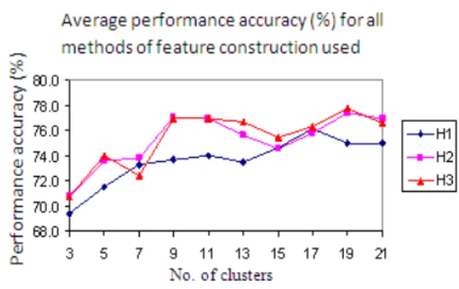
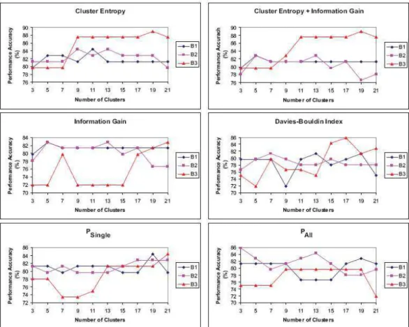
Figure 6 and 7 shows the average performance accuracy of the J48 classifier for all feature construction methods studied using the Mutagenesis (B1, B2, B3) and Hepatitis (H1, H2, H3) databases with k = 3,5,7,9, 11,13,15,17,19,21. Generally, the number of clusters has no implications on the average performance accuracy of the classification tasks, for datasets B1 and B2. In contrast, the results show that for datasets B3, H1, H2 and H3, the average performance accuracy tends to increase when the number of clusters increases. Figure 8 and 9 show the performance accuracies of the J48 classifier for different methods of features construction used to generate patterns for the Mutagenesis (B1, B2, B3) and Hepatitis (H1, H2, H3)
datasets, with different values of k. In the Mutagenesis B1 and B2 datasets, the size of the cluster has no implications on the predictive accuracy when using the features constructed from the CE, CE_IG, IG and DBI genetic-based feature construction algorithms. As the number of clusters increases, the predictive accuracy tends to stay steady or to decrease as shown in Fig. 8.
For the Hepatitis (H1, H2, H3) and Mutagenesis (B3) datasets, the predictive accuracy results of the J48 classifier are higher when the number of cluster k is relatively big (17≤k≤19) when using the constructed features from the CE genetic-based feature construction algorithm. In contrast, the predictive accuracy results of the J48 classifier for the datasets (Hepatitis H1, H2, H3 and Mutagenesis B3) are higher when the number of clusters k is relatively small (9≤k≤11) and the features used are constructed by the PSingle and PAll methods.
Fig. 6: The average performance accuracy of J48 classifier for all feature construction methods tested on Mutagenesis datasets B1, B2 and B3
874
Fig. 8: Performance accuracy of J48 classifier for Mutagenesis datasets B1, B2 and B3 The arrangement of the objects within the clusters can
be considered as a possible cause of these results. The feature space for the PSingle method is too large and thus
this feature space does not provide clear differences that discriminates instances[33,34]. On the other hand, the feature space is restricted to a small number of specific patterns only when we apply the PAll method to
construct the patterns. With PAll method, the task of
inducing similarities for instances is difficult and thus it is difficult to arrange related objects close enough to each other[33,34]. As a result, when the number of clusters is too small or too large, each cluster may have a mixture of unrelated objects and this leads to lower predictive accuracy results. On the other hand, when the patterns are produced by using the CE or IG genetic-based feature construction algorithms, the feature space is constructed in such a way that related objects can be arranged closely to each other. As a result, the performance accuracy of the J48 tends to increase when the number of clusters increases. It is shown in the experimental results that when the descriptive accuracy of the summarized data is improved, the predictive
accuracy is also improved. In other words, when the choice of newly constructed features minimizes the cluster entropy, the predictive accuracy of the classification task also improves as a results.
875
Fig. 9: Performance accuracy of J48 classifier for Hepatitis datasets H1, H2 and H3
Table 5: Indices of Attributes in Mutagenesis datasets (B1, B2, B3)
Indices B1 B2 B3
1 Element1 Element1 Element1
2 Element2 Element2 Element2
3 Type1 Type1 Type1
4 Type2 Type2 Type2
5 Bond Bond Bond
6 - Charge1 Charge1
7 - Charge2 Charge2
8 - - logP
9 - - ∈LUMO
Table 6: Features constructed for Mutagenesis datasets (B1, B2, B3)
Datasets CE CE_IG
B1 [2, 4],[1, 3, 5] [3, 4],[1, 2, 5] B2 2, 4, 5],[1, 3, 6, 7] [3, 4],[1, 2, 5, 6, 7] B3 [1, 3, 9],[2, 6, 8],[4, 5, 7] [1, 7],[5, 6],[3, 9],[2, 4, 8]
IG DBI
--- --- B1 [3, 4],[1, 2, 5] [4, 5],[1, 2, 3]
B2 [3, 4],[1, 2, 5, 6, 7] [1, 3],[4, 5],[2, 6, 7] B3 [1, 7],[5, 6],[3, 9],[2, 4, 8] [5, 6],[3, 9],[7, 8],[1, 2, 4]
For instance, by using the CE fitness function, the values for Element2 and Type2 are coupled together (in
B1 and B2) to form a single pattern that is used in the clustering process. These values can be used to represent the characteristics of the clusters formed. On the other hand, by using the IG alternative, the values for Type1 and Type2 are coupled together (in B1 and
B2) to form a single pattern that will be used in the clustering process. Based on Table 6, it can be determined that when CE is used, attributes are coupled more appropriately compared to the other alternatives. For instance, by using DBI, the values for Type2 and
Bond are coupled together to form a single pattern and these attributes are not appropriately coupled.
876 experiments. We evaluated the quality of the newly constructed features by comparing the predictive accuracy of the J48 classifier obtained from the data with patterns generated using these newly constructed features with the predictive accuracy of the J48 classifier obtained from the data with patterns generated using the original attributes.
In summary, based on the results shown in Table 3, the following conclusions can be made:
• Setting the total Cluster Entropy (CE) as the feature scoring function to determine the best set of constructed features can improve the overall predictive accuracy of a classification task
• Better performance accuracy can be obtained when using an optimal number of clusters to summarize the data stored in the non-target tables
• The best performance accuracy is obtained when the number of clusters is in the higher end of the range (19). Therefore, it can be assumed that performing data summarization with a relatively optimal number of clusters would result in better performance accuracy on the classification task
CONCLUSION
In the process of learning a given target table that has a one-to-many relationship with another non-target table, a data summarization process can be performed to summarize records stored in the non-target table that correspond to records stored in the target table. In the case of a classification task, part of the data stored in the non-target table can be summarized based on the class label or without the class label. To summarize the non-target table, a record can be represented as a vector of patterns and each pattern may be generated from a single attribute value (PSingle) or a combination of
several attribute values (PAll). These objects are then
clustered or summarized on the basis of these patterns. In this study, methods of feature construction for the purpose of data summarization were studied. A genetic-based feature construction algorithm has been proposed to generate patterns that best represent the characteristics of records that have multiple instances stored in the non-target table.
Unlike other approaches to feature construction, this paper has outlined the usage of feature construction to improve the descriptive accuracy of the proposed data summarization approach (DARA). Most feature construction methods deal with problems to find the
best set of constructed features that can improve the predictive accuracy of a classification task. This study has described how feature construction can be used in the data summarization process to get better descriptive accuracy, and indirectly improve the predictive accuracy of a classification task. In particular, we have investigated the use of Information Gain (IG), Cluster Entropy (CE), Davies-Bouldin Index (DBI) and a combination of Information Gain and Cluster Entropy (CE-IG) as the fitness functions used in the genetic-based feature construction algorithm to construct new features.
It is shown in the experimental results that the quality of summarized data is directly influenced by the methods used to create patterns that represent records in the (n×p) TF-IDF weighted frequency matrix. The results of the evaluation of the genetic-based feature construction algorithm show that the data summarization results can be improved by constructing features by using the Cluster Entropy (CE) genetic-based feature construction algorithm.
REFERENCES
1. Alfred, R. and D. Kazakov, 2006. Data Summarization Approach to Relational Domain Learning Based on Frequent Pattern to Support the Development of Decision Making. Proceeding of the 2nd International Conference on Advanced Data Mining and Applications, Aug. 14-16, Xi'an, China, pp: 889-898.
2. Blockeel, H. and L. Dehaspe, 1999. Tilde and Warmr User Manual, Version 2.0, Katholieke Universiteit, Leuven.
http://www.cs.kuleuven.ac.be/~ml/Doc/TW_User/ 3. Lavrac, N. and P.A. Flach, 2001. An extended
transformation approach to inductive logic programming. ACM Trans. Comput. Logic, 2: 458-494. DOI: 10.1145/383779.383781
4. Salton, G., A. Wong and C.S. Yang, 1975. A vector space model for automatic indexing. Commun., ACM, 18: 613-620.
5. Cubero, J.C., J.M. Medina, O. Pons and M.A. Vila, 1999. Data summarization in relational databases through fuzzy dependencies. Int. J. Inform. Sci., 121: 233-270. DOI: 10.1016/S0020-0255(99)00104-8
877 7. Kirsten, M. and S. Wrobel, 1998. Relational
distance-based clustering. Proceeding of the 8th International Conference on Inductive Logic Programming, July 22-24, Springer, Madison, Wisconsin, pp: 261-270.
8. Dietterich, T.G. and R.S. Michalski, 1981. Inductive learning of structural descriptions: Evaluation criteria and comparative review of selected methods. Artif. Intel., 16: 257-294. 9. David, W.A., 1991. Incremental constructive
induction: An instance-based approach. http://www.pubzone.org/dblp/conf/icml/Aha91 10. Pagallo, G. and D. Haussler, 1990. Boolean feature
discovery in empirical learning. Mach. Learn., 5: 71-99. DOI: 10.1023/A:1022611825350
11. Hu, Y. and Dennis F. Kibler, 1996. Generation of attributes for learning algorithms. Proceeding of the 1996 13th National Conference on Artificial Intelligence, Aug. 04-08, Portland, Oregon, USA., pp: 806-811.
12. Hu, Y., 1998. A genetic programming approach to constructive induction. Proceeding of the 3rd Annual Genetic Programming Conference, July 22-25, Morgan Kauffman, Madison, Wisconsin, pp: 146-157.
13. Otero, F.E.B., M.M.S. Silva, A.A. Freitas and J.C. Nievola, 2003. Genetic Programming For Attribute Construction in Data Mining. EuroGP, Morgan Kaufmann Publishers Inc., San Francisco, CA, USA., ISBN:1-55860-878-8, pp: 384-393. 14. Bensusan, H. and I. Kuscu, 1996. Constructive
Induction using Genetic Programming. Proceeding of the Evolutionary Computing and Machine Learning Workshop July 1996, Bari, Italy.
15. Zheng. Z., 1996. Effects of Different Types of New Attribute on Constructive Induction. Proceedings of the 8th International Conference on Tools with Artificial Intelligence, (ICTAI’96), IEEE Computer Society, Washington DC., USA., pp: 254-257.
16. Zheng, Z., 2000. Constructing X-of-N attributes for decision tree learning. Mach. Learn., 40: 35-75. 17. Quinlan, R.J., 1993. C4.5: Programs for Machine
Learning. Morgan Kaufmann, San Francisco, CA., USA., ISBN:1-55860-238-0, pp: 302.
18. Koller, D. and M. Sahami, 1996. Toward optimal feature selection.
http://ilpubs.stanford.edu:8090/208/1/1996-77.pdf 19. Amaldi, E. and V. Kann, 1998. On the
approximability of minimizing nonzero variables or unsatisfied relations in linear systems. Theor. Comput. Sci., 209: 237-260.
20. Freitas, A., 2001. Understanding the crucial role of attribute interaction in data mining. Artif. Intel. Rev., 16:177-199.
21. Shafti, L.S. and E. Perez, 2003. Genetic approach to constructive induction based on non-algebraic feature representation. Lecture Notes Comput. Sci., 2779: 599-610. DOI: 10.1007/b13240
22. Michalewicz, Z., 1994. Genetic Algorithms Plus Data Structures Equals Evolution Programs. 2nd Edn., Springer-Verlag, New York, Secaucus, NJ., USA., ISBN:0387580905, pp: 340.
23. Holland, J., 1992. Adaptation in Natural and Artificial Systems. 1st Edn., MIT Press, ISBN:0-262-08213-6, pp: 211.
24. Vafaie, H. and K. DeJong, 1998. Feature space transformation using genetic algorithms. IEEE Intell. Syst., 13: 57-65. DOI: 10.1109/5254.671093 25. Koza, J.R., 1994. Genetic programming: On the programming of computers by means of natural selection. Stat. Comput., U. K., 4: 191-198. http://www.genetic-programming.com/SCJ.ps 26. Krawiec, K., 2002. Genetic programming-based
construction of features for machine learning and knowledge discovery tasks. Genet. Programm. Evolv. Mach., 3: 329-343. DOI: 10.1023/A:1020984725014
27. Davies, D.L. and D.W. Bouldin, 1979. A cluster separation measure. IEEE Trans. Patt. Anal. Mach. Intel., 1: 224-227.
28. Shannon, C.E., 1948. A mathematical theory of communication. Bell Syst. Tech. J., 27: 379-423, 623-656.
29. Wiener, N., 2000. Cybernetics Or Control and Communication in Animal and the Machine. 2nd Edn. MIT Press, Cambridge, MA, USA, ISBN-10: 026273009X, pp: 212.
30. Berger, W.H. and F.L. Parker, 1970. Diversity of planktonic foraminifera in deep-sea sediments. Science, 168: 1345-1347.
31. Srinivasan, A., S. Muggleton, M.J.E. Sternberg and R.D. King, 1996. Theories for mutagenicity: A study in first-order and feature-based induction. Artif. Intel., 85: 277-299.
32. Ian, H.W. and E. Frank, 1999. Data mining: Practical machine learning tools and techniques with Java implementations. 2nd Edn., Morgan Kaufmann, ISBN: 0-12-088407-0, pp: 525.
33. Kramer, S., 2000. Relational Learning versus Propositionalisation. AI Commun., 13: 275-276. 34. Perlich, C. and F.J. Provost, 2006.