www.atmos-chem-phys.net/11/11761/2011/ doi:10.5194/acp-11-11761-2011
© Author(s) 2011. CC Attribution 3.0 License.
Chemistry
and Physics
Novel application of satellite and in-situ measurements to map
surface-level NO
2
in the Great Lakes region
C. J. Lee1, J. R. Brook2, G. J. Evans1, R. V. Martin3,4, and C. Mihele2
1Southern Ontario Centre for Atmospheric Aerosol Research, Department of Chemical Engineering and Applied Chemistry,
University of Toronto, Toronto, Ontario, Canada
2Air Quality Research Division, Science and Technology Branch, Environment Canada, Downsview, ON, Canada 3Department of Physics and Atmospheric Science, Dalhousie University, Halifax, Nova Scotia, Canada
4Harvard-Smithsonian Center for Astrophysics, Cambridge, MA, USA
Received: 12 March 2011 – Published in Atmos. Chem. Phys. Discuss.: 21 June 2011 Revised: 28 October 2011 – Accepted: 10 November 2011 – Published: 24 November 2011
Abstract. Ozone Monitoring Instrument (OMI) tropospheric
NO2vertical column density data were used in conjunction
with in-situ NO2concentrations collected by permanently
in-stalled monitoring stations to infer 24 h surface-level NO2
concentrations at 0.1◦(∼11 km) resolution. The region ex-amined included rural and suburban areas, and the highly in-dustrialised area of Windsor, Ontario, which is situated di-rectly across the US-Canada border from Detroit, MI. Pho-tolytic NO2 monitors were collocated with standard NO2
monitors to provide qualitative data regarding NOz
interfer-ence during the campaign. The accuracy of the OMI-inferred concentrations was tested using two-week integrative NO2
measurements collected with passive monitors at 18 loca-tions, approximating a 15 km grid across the region, for 7 consecutive two-week periods. When compared with these passive results, satellite-inferred concentrations showed an 18 % positive bias. The correlation of the passive mon-itor and OMI-inferred concentrations (R=0.69, n=115) was stronger than that for the passive monitor concentrations and OMI column densities (R=0.52), indicating that using a sparse network of monitoring sites to estimate concentra-tions improves the direct utility of the OMI observaconcentra-tions. OMI-inferred concentrations were then calculated for four years to show an overall declining trend in surface NO2
con-centrations in the region. Additionally, by separating OMI-inferred surface concentrations by wind direction, clear pat-terns in emissions and affected down-wind regions, in partic-ular around the US-Canada border, were revealed.
Correspondence to: C. J. Lee ([email protected])
1 Introduction
Nitrogen oxides (NOx), composed of nitric oxide (NO) and
nitrogen dioxide (NO2) are an important family of
atmo-spheric pollutants (NOx=NO+NO2). The main source of
NOx in Ontario, Canada is transportation, with a smaller
component originating from electricity generation and indus-trial processes (MoE, 2008). Other sources of NOxinclude
soil and lightning. NO2has been used as a marker for
vehi-cle emissions and has thereby been associated with adverse human health effects (Brook et al., 2007; Jerrett et al., 2009; Clark et al., 2010; Lenters et al., 2010). In the province of Ontario, Canada, the government guideline exposure limit for NO2is 100 ppb averaged over 24 h and 200 ppb averaged
over 1 h. Despite the association of NO2with adverse health
outcomes, and its utility as a marker for traffic and/or com-bustion pollution, NO2monitoring networks remain sparse.
NO2is commonly measured by chemiluminescence (CL)
monitors which work by reducing NO2to NO and
measur-ing the light produced by titratmeasur-ing the NO with O3. There
are a number of methods for reducing the NO2, the most
common being a heated molybdenum surface, which be-comes oxidized to MoO2 and MoO3 and must be
peri-odically recharged. We will refer to this type of mon-itor as MoO. These monmon-itors are known to suffer from interference due to other oxidized nitrogen species NOz
(NOz=HNO3+HONO+N2O5+RONO2+...), since the
heated molybdenum surface exhibits low selectivity (Winer et al., 1974; Steinbacher et al., 2007). This interference can especially be a problem in rural areas with low NO2
concen-trations and high NOzdue to aged air masses or high organic
photolytic monitors operate on essentially the same principle as the MoO-CL monitors, however, the NO2 is reduced by
applying intense light at∼420 nm which is specific to NO2
and therefore is expected to produce almost no interference from other oxidized nitrogen species.
Due to the low relative per-monitor cost, NO2 has also
been measured using networks of passive monitors. For ample, the networks have been used to assess human ex-posure to traffic related air pollution at high spatial resolu-tion (Jerrett et al., 2009). These passive monitors consist of a chemically treated filter pad placed in a protective housing and exposed to ambient air for a period of time, usually two or more days. At the end of the sampling period, the filter is removed and the treatment is dissolved off the filter and an-alyzed using ion chromatography. Although the filters them-selves are inexpensive, the method is labour intensive. As well, since there are no pumps, the exposure, and therefore the collection efficiency, is influenced by local meteorology. Beginning with the Global Ozone Monitoring Experi-ment (GOME) in 1995, satellite-based spectroscopic mea-surements of atmospheric NO2have been taken by a series
of instruments (Bovensmann et al., 1999; Burrows et al., 1999; Levelt et al., 2006). The Ozone Monitoring Instru-ment (OMI), launched in 2004 aboard the Aura satellite, has provided near daily-global NO2column measurements
at unprecedented spatial resolution. Many recent works have compared OMI NO2 columns with measurements provided
by in situ surface monitors (Kramer et al., 2008; Boersma et al., 2009), long-path surface measurements (Kramer et al., 2008) and in situ aircraft measurements (Bucsela et al., 2008). Recent validation studies indicate that biases in the satellite retrievals remain and must be addressed when in-terpreting the data (Hains et al., 2010; Herron-Thorpe et al., 2010; O’Byrne et al., 2010; Lamsal et al., 2010). It is also important to note that a number of different data products with significant differences exist, adding to the complexity of comparisons between OMI and in-situ data.
Lamsal et al. (2008) used GEOS-Chem, a global chem-ical transport model (CTM), to infer ground level concen-trations from OMI NO2 data and showed good agreement
between OMI overpass measurements and 2 h averages from a large network of ground monitors over the continental US and Canada with a mean difference of −18 % (urban) to 11 % (rural) between OMI inferred concentrations and cor-rected surface monitor data during the summer and fall sea-sons. Other studies such as Boersma et al. (2009) and Russell et al. (2010) have examined spatial and temporal characteris-tics of NO2over smaller regions such as Israel and
Califor-nia. Additionally, satellite NO2measurements were found to
agree well with surface-level column measurements taken by MAX-DOAS as part the BAQS-met campaign (Halla et al., 2011). These analyses indicate that insight into the spatial distribution of ground-level NO2at a regional-to-local scale
on the Earth’s surface can be achieved with satellite remote sensing.
These high resolution OMI column density measurements also have been applied to constrain emissions. For example, Boersma et al. (2007) conducted an inversion using GEOS-Chem to infer emissions for the Eastern United States and Mexico and differences between these OMI-constrained top-down inventories and the US EPA National Emissions In-ventory for 1999 (NEI99) were further used to infer changes over time to emissions from specific sectors. This was pos-sible due to the geographic separation of the different sec-tors’ emissions and the fine spatial resolution of the OMI-constrained top-down inventories. OMI column data has also been used to help verify and develop a regional chemistry model with 15 km resolution around the state of California (Kim et al., 2009). The weekend effect was also observed and contrasted between different cities in California using OMI vertical column densities from multiple years averaged on a 0.025◦(∼3 km) grid (Russell et al., 2010).
High-resolution estimates of surface concentrations can provide a number of contributions to air quality research:
– to closely examine urban impacts on surrounding rural
regions,
– to improve estimates of chronic human and ecosystem
exposure patterns,
– to look at transboundary flow of NOx which has been
used as a combustion tracer when close to the source of combustion,
– to evaluate high-resolution air quality models (e.g.,
Makar et al., 2010).
The BAQS-met campaign was conducted in Southwest-ern Ontario, around the Windsor-Detroit area, from 1 June to 10 September 2007. The main goal of BAQS-met was to study the effects of transboundary air pollution and the Great Lakes meteorology on local air quality. The area was chosen due to its unique geography (i.e. frequent influence of lake breezes), proximity to the US-Canada border and lo-cal industry. A comprehensive suite of measurements, which have been described in other papers in this special issue (e.g., Levy et al., 2010) and included a diverse and relatively dense array of surface NO2measurements, provided a unique
op-portunity to develop and evaluate OMI-derived surface NO2
concentration estimates.
In situ NO2routine monitoring data are publicly available.
However, these monitors are sparsely-spaced, point measure-ments. It is therefore difficult to provide an accurate repre-sentation of NO2concentrations in between monitoring
sta-tions. The objectives of the work in this paper are thus to develop an approach to use OMI tropospheric column data to estimate spatially resolved surface NO2concentrations at
As discussed above, a major contribution of previous work in this area was the use of a CTM to estimate a surface-concentration-to-column-density ratio which was applied to satellite NO2columns for this purpose (Lamsal et al., 2008).
We hypothesized that this ratio could be calculated using publicly available data from a network of permanent surface monitoring stations in place of the CTM, in regions with suf-ficient ground-based monitors. This approach has the advan-tage of simplicity since it is not dependent upon CTM runs. Another potential advantage to this method is the empirical nature by which it is calculated, making it less sensitive to the OMI data product used. This claim is explained further in Sect. 2.3.
Because of the nature of the BAQS-met campaign setup, several important facets of our hypothesis could be examined and are reported in this paper. The estimated surface NO2
results were compared with passive NO2measurements
ob-tained at 18 locations for each of 7 sampling periods. Since the passive sites were spaced as closely as 15 km and were not used to calculate the ratio (i.e., were independent), they were well-suited for determining the accuracy of the esti-mated concentrations on a spatial scale not yet examined, across a variety of land-use types spanning from urban to rural locations. The collocated conventional and photolytic NO2 monitors allowed for quantification of the NOz
inter-ference known to impact conventional measurements. Ad-ditionally, it was possible to examine the diurnal patterns in the interference and to assess the impact of these pat-terns on the comparison of the 14-day integrated passive NO2
with the 14-day average OMI NO2based upon the midday
overpasses. Finally, because of the additional rural chemi-luminescence monitoring provided during the campaign, the value of these more spatially representative rural monitoring sites for improving the exploitation of the freely available OMI satellite observations could be highlighted.
To the best of our knowledge, the simple approach we develop and evaluate here for combining in-situ data from permanent monitoring stations with high-resolution satellite data to obtain high-resolution (∼11 km) estimates of long-term average surface NO2 concentration maps has not been
considered before. In addition, the region covered and the 15 km spacing of the passive monitors allowed for an un-precedented surface NO2 dataset against which to compare
the maps generated using this novel method. Furthermore, the use of two-week passive samplers for evaluation provides a baseline which is expected to be more representative of chronic human-exposure conditions, therefore increasing the relevance of this study to the health research community.
2 Measurements of Windsor and Southwest Ontario area NO2
Windsor, Ontario, is located at the southwestern tip of the province of Ontario. It is bordered by the Detroit River on the
west side and Lake St. Clair to the north, as well as Lake Erie several km to the south. This type of waterfront geography can have effects on NO2concentrations due to lake breezes
(Arain et al., 2009). Across the Detroit river lies Detroit, MI. Both cities are known for their auto industry. The Windsor metropolitan area has a population of 323 000 and an area of 1023 km2, while the City of Windsor has a population of 216 500 and occupies an area of 147 km2(Statistics Canada, 2006). Southeast Michigan, including Detroit-Warren-Flint, is the eleventh most populous combined statistical area in the US with a population of 5 300 000 and an area of 15 000 km2 (US Census Bureau).
2.1 High-time resolution measurement by chemiluminescence
The Ontario Ministry of the Environment (MoE) operates a permanent monitoring network which includes 2 stations within Windsor and one in Chatham (Fig. 1). Due to their proximity to the campaign area, MoE permanent monitoring sites in Sarnia, at the Southern end of Lake Huron, and Lon-don, approximately 150 km Northeast of Windsor, were also included (Fig. 2). As well, during the intensive campaign pe-riod (20 June–10 July 2007) 3 additional chemiluminescence (CL) monitors were set up at Harrow and Ridgetown, on the North shore of Lake Erie approximately 40 km and 100 km from Windsor, respectively, and on Pelee Island, a 42 km2 island approximately 50 km Southeast of Harrow in Lake Erie (Fig. 1). The monitors operated by MoE were Thermo TE42C instruments which provide NO, NO2and NOx.
Mea-surements were averaged to 1 h to match the data available from the permanent MoE network.
To evaluate the potential interference from non-NO2
ox-idized nitrogen species (Steinbacher et al., 2007; Ord´o˜nez et al., 2006; Lamsal et al., 2008), 3 CL monitors (TE42C and TE42CTL) were deployed by Environment Canada for the duration of the campaign (1 June 2007 to 11 September 2007). One of these monitors was located at Bear Creek, col-located with a MoO-CL monitor; one was col-located at Harrow; and one (which was not used in this analysis) was onboard the Environment Canada mobile platform, CRUISER. These CL monitors were each equipped with a photolytic converter (Droplet Measurement Technologies, blue light converter) and an external molybdenum converter. By selecting ambient air, photolytically converted air, or molybdenum converted air, true NO2could be reported by subtracting NO from the
measured post-conversion NO and applying the conversion efficiency of NO2to NO. One minute concentrations for NO,
NO2 and NOy (NOy=NOx+NOz) were provided by
run-ning a 1 min cycle with the three above channels and 2 inter-nal zeros.
It is important to highlight that the method for measur-ing NOyis exactly the same as the method commonly used
for measuring NO2with the exception that in traditional
Fig. 1. NO2monitoring sites for the 2007 BAQS-Met campaign.
Passive monitoring locations are denoted by black-and-white cir-cles. High-time resolution chemiluminescence monitor locations are marked by yellow bubbles with text labels. Chatham, Wind-sor West and WindWind-sor Downtown were Ontario Ministry of the En-vironment (MoE) permanent monitoring stations. Harrow, Pelee and Ridgetown also had monitors operated by MoE from 20 June to 10 July. Harrow had a photolytically converted chemilumines-cence monitor operated by Environment Canada from 1 June to 10 September and Bear Creek had both molybdenum and photolyt-ically converted monitors operated by Environment Canada for the same period. Two additional MoE permanent monitoring station not shown by this map were also used (Sarnia and London).
monitor. The NOzinterference in MoO NO2measurements
is therefore a product of the conversion efficiency of the con-stituent species of NOz as well as their respective line loss
parameters (HNO3is particularly noted for line losses,
Stein-bacher et al., 2007). In the NO-NO2-NOy setup used for
measuring the interference, the MoO converter was applied before the sampling line and NOymeasurement was
depen-dent only on the conversion efficiencies of the species.
2.2 Measurement by passive monitor
A network of passive NO2monitors was deployed at 18
lo-cations (Fig. 2). These sites were part of the Mesonet study (Levy et al., 2010) and were chosen to closely match the En-vironment Canada Global EnEn-vironmental Multiscale model (Makar et al., 2010) meteorological forecast 15 km model grid in the region (every grid point where possible, alternate grid points in other locations). In some cases the need to ac-cess the monitors on a regular basis caused small deviations from the model grid. Weatherproof housings were anchored to the Mesonet towers at the sampling sites. These housings were designed to allow ambient air contact with the monitors while keeping out rain.
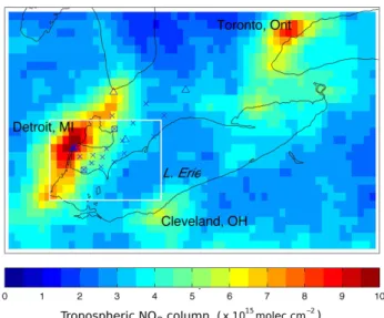
Fig. 2. Campaign average NO2column in Southwestern Ontario.
BAQS-met passive monitoring sites are marked by Xs, triangles represent permanent MoE molybdenum converted NOxmonitoring
locations and squares denote locations of EC photolytically con-verted NOxmonitors during the campaign. White rectangle outlines
area encompassed by Fig. 1.
Further, since the filters needed to be collected for analy-sis and replaced with fresh samplers manually, site locations were selected with the criterion that all sites could be reached in a single day. The intention was to provide consistent sam-pling period start and end dates across all samsam-pling periods. However, this was not always possible and some sites saw collection and replacement up to two days before others, al-though most sites were collected and replaced on the same day in most cases. In total, there were 115 passive samples collected: the first 6 periods (31 May to 22 August) had 17 simultaneous sampling sites and the final period (23 August to 6 September) had 13 sampling sites. On average, 70 % of the filters were collected on a single day, thus maximizing temporal overlap for the two-week period. For sampling pe-riods 1 and 3 through 7, all filters were collected within a 2 day period; for sampling period 2, all filters were collected within a 2 day period, except one filter which was collected 2 days later than the first.
unexposed filters, carried to and from the sampling locations during the campaign, were used for background/blank cor-rection.
2.3 Satellite remote sensing
The OMI instrument is onboard the Earth Observing Sys-tem (EOS) Aura satellite which is in a sun-synchronous orbit with south-north Equator crossing of 13:45 LT (Levelt et al., 2006). OMI is carried aboard the Earth Observing System. With a wide field-of-view and sun-synchronous orbit, the in-strument was designed to provide daily coverage across most of the globe. The sensor observes 60 pixels which together cover a swath 2600 km wide, perpendicular to the direction of travel. The satellite travels at approximately 7 km s−1 ground speed and each exposure is roughly 2 s long, resulting in each row covering 13 km on the ground in the along-track direction. Across track, pixels are 24 km wide at nadir, but due to geometry, nearer the edge of the swath, pixels can be as wide as 150 km. Recently, obstruction of parts of the sen-sor has limited measurements slightly, removing as many as 18 pixels out of the 60.
Two commonly used, publicly available data products generated from the raw data collected by OMI are: the Standard Product (SP) provided by NASA (Bucsela et al., 2006, http://disc.sci.gsfc.nasa.gov/Aura/data-holdings/OMI/ omno2 v003.shtml), and the DOMINO Product provided by the Tropospheric Emissions Monitoring Internet Service (TEMIS) (Boersma et al., 2007, http://temis.nl/airpollution/ no2.html). Both data products begin by using the DOAS al-gorithm to fit the absorption spectrum of NO2 to the
mea-sured spectrum of backscattered 405 to 465 nm solar radia-tion (Boersma et al., 2007). The contriburadia-tion of stratospheric NO2 is then removed (Bucsela et al., 2006; Boersma et al.,
2007). The air mass factor (AMF) accounts for viewing geometry and light-scattering interferences such as clouds; this AMF is applied to convert the measured slant columns into tropospheric vertical column densities. It is these con-versions that introduce the most uncertainty in the reported vertical columns over polluted areas (Boersma et al., 2007, 2004; Martin et al., 2002).
The use of in situ data to determine the surface-to-column NO2 relationship makes this analysis insensitive to
poten-tial bias in the OMI NO2data. Starting with the DOMINO
product, a tropospheric slant column destriping process was used to remove scan-angle dependent bias (Celarier et al., 2008; Lamsal et al., 2010), using a 24 h history to compute single-scan position biases. Pixels with cloud radiance frac-tions greater than 0.3 were rejected, as were pixels near the edge of the swath (width>50 km). The resulting vertical col-umn densities easily identified the urban areas as major NOx
sources (Fig. 2).
Whereas in situ measurements are true surface measure-ments, OMI tropospheric NO2vertical column density
mea-surements include both the surface-level NO2and its vertical
distribution through the tropospheric column. This distribu-tion depends on the chemical lifetime of NOx, the
partition-ing of NOxinto NO and NO2, layering of the atmosphere and
the dispersion of NOxduring vertical mixing. Lamsal et al.
(2008) inferred surface-level NO2 concentrations (S) from
OMI tropospheric vertical column densities () by applying the ratio of surface-level NO2concentrations (SG) to
verti-cal column densities (G) calculated using the GEOS-Chem
global CTM:
S= SG
G
× (1)
In order to obtain surface concentrations without the use of a CTM, we determined the spatial average ratio of in situ surface concentration (S) to OMI columns (), coincident with surface monitoring stations, over the region (Eq. 2),
S= S
−BG
×(−BG) (2)
whereBGis the background OMI NO2column as described
in the subsequent paragraph.
To account for the larger fractional contribution of the free troposphere in areas with low surface concentrations, all pix-els (after filtering) in the region contained by the boundary of Fig. 2 were sorted by column density for each overpass. The lowest decile value (i.e., the value separating the bottom 10 % of the data from the remaining 90 % of pixels) was subtracted from every pixel in the overpass. This allowed for the free-tropospheric component to be accounted for (BGin Eq. 2),
while limiting sensitivity to the uncertainty of any single pixel. The mean value of the free-tropospheric column dur-ing the campaign period was 0.8×10¹⁵molec cm−2. This process did result in negative (i.e., below detection) values, but they were typically small and constrained to the north-ernmost areas of the region.
Each single-pixel measurement carries with it an uncer-tainty due to the spectral fitting, surface albedo, cloud cover and air mass factor. This uncertainty can reach up to 40 % in heavily polluted areas (Boersma et al., 2007), including the locations of some of the high-time resolution in situ moni-tors used to calculate the surface-to-column ratio. In addi-tion to this, an OMI pixel is an average over a large area on the surface of the Earth while the in situ monitors measure at a specific location which is not necessarily representative of the entire pixel area against which is being compared. We therefore generated an average surface-to-column ratio for the entire region by averaging the ratios observed at several surface monitoring stations. Implicit to this approach was the assumption that this ratio varies temporally (i.e., day-to-day) but not spatially across the region on any given day. The error in this assumption is discussed in Sect. 3.3.1.
this average ratio ( S
−BG
in Eq. 2) to provide a region-wide snapshot of surface NO2 concentrations at overpass time.
This procedure was analogous to Eq. (4) from Lamsal et al. (2008), which also accounts for the contribution of the free troposphere. Equation (4) from Lamsal et al. (2008) also provides higher resolution than the available GEOS-Chem 2◦×2.5◦ resolution using a ratio of local OMI columns to the average OMI column for the entire grid cell. This sug-gests that by using a single ratio for the entire region for each overpass, an error of up to±35 % is introduced in rural areas. From Eq. (2), it can been seen that the use of in situ data to determine the surface-to-column NO2relationship makes
this analysis insensitive to potential bias in the OMI NO2
data. Because OMI column densities appear in both the nu-merator and the denominator, any bias present in the partic-ular retrieval used would be expected to cancel out. As an example, it has been suggested that the SP is biased low in the winter (Lamsal et al., 2008). If the surface-to-column ra-tio is calculated using the (assumed, in this case, unbiased) modeled surface concentration and modeled column density, the inferred surface values from these low OMI columns will also be biased low. However, by calculating the ratio using the observed OMI columns, assuming the in-situ measured surface concentration is the same as the modeled surface con-centration, the surface-to-column ratio will be greater than the modeled surface-to-column ratio which will increase the final inferred surface concentrations.
For comparison of OMI column densities and surface con-centrations with long-term time-averaged passive monitor re-sults, OMI measurements were resampled on a 0.1◦×0.1◦ grid. Each grid cell was then given a weight proportional to the inverse of the area of the pixel which contained that grid cell. This had the effect of giving near-nadir pixels higher weight than pixels closer to the swath edge. These regrid-ded measurements were then averaged over two weeks us-ing these weights, providus-ing a long-term average to com-pare with in situ passive monitor measurements. Although this weighting scheme has also been used with a squared-uncertainty term (Wenig et al., 2008), it was found that inverse-area-alone weighted values used here differed from inverse-area, inverse-squared-uncertainty weighted values by less than 3 % for the 2-week averages over the campaign pe-riod.
3 Results and discussion
3.1 Characterising surface NO2
3.1.1 Spatial and temporal patterns inferred from chemiluminescence monitor data
NO2 concentrations were found to vary both spatially and
temporally. The hourly and daily concentrations of NO2
showed moderate to weak correlations between the sites
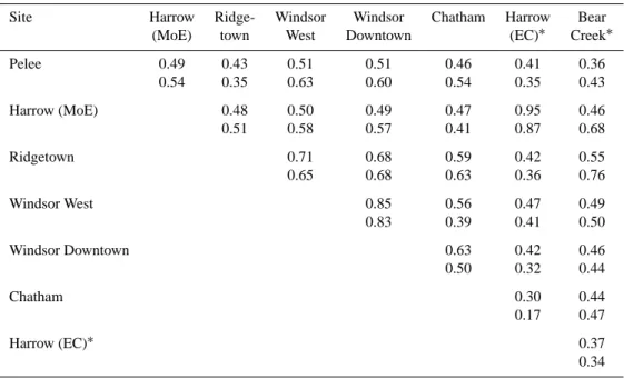
over the duration of the campaign (Table 1). This compar-ison is important to help identify potential sources of pollu-tion affecting different areas of the campaign region, which spans urban, rural and industrial areas. Ridgetown showed a relatively high correlation with the urban sites (∼0.7), which was surprising because Ridgetown is over 100 km from the urban and industrial centre of Windsor. However, the Ridgetown measurement site was 5 km from highway 401, a major provincial highway in the region leading di-rectly to the Ambassador Bridge border crossing in Windsor. This relatively strong correlation despite the spatial separa-tion implied that 401 traffic was an important source in both of these areas.
NO2 concentrations varied diurnally and day-to-day at
both the urban (Windsor) and rural (Harrow, Bear Creek) sites (Fig. 3). Peak concentrations for Windsor occurred be-tween 06:00 and 10:00 a.m. (local standard time) on most days, while these morning rush-hour peaks were sometimes delayed at the rural sites downwind. Variation between sites was greater than week-to-week variations in same-site NO2 concentrations (Table 2). The largest between-site
ra-tio in the median weekly concentrara-tion was over 4 (Windsor Downtown had a weekly median concentration of 13.6 ppb while Peelee had a weekly mean of only 2.9 ppb) whereas the largest ratio between maximum and minimum weekly concentrations at a single site was less than 2 (Peelee had the highest ratio with a maximum weekly concentration of 3.1 ppb and a minimum of 1.7 ppb). In contrast, daily aver-ages varied about as much at a given site as they did between sites. This indicated that spatial distributions remain fairly stable over the region, even though local events may briefly increase the spatial heterogeneity. This result is important for high spatial resolution interpretation of satellite remote sens-ing data because these methods take advantage of differences in the daily footprint of the instrument overpass to extract long-term patterns in spatial air pollution distributions.
3.1.2 Passive monitor results
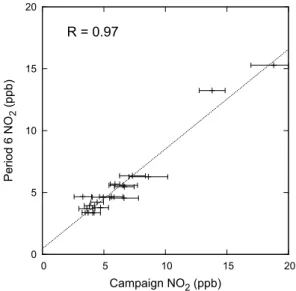
Campaign average NO2measurements recorded at the
pas-sive monitoring sites ranged from a minimum site average of 3.3 ppb (rural) to a maximum of 18.8 ppb (urban). The pas-sive monitors also revealed that over the long-term the mag-nitude of the spatial variability was greater than the magni-tude of the differences between time periods at a given loca-tion. This is exemplified in Fig. 4, comparing the concentra-tions measured at each location for sampling period 6 (7 Au-gust to 21 AuAu-gust) to the campaign average concentration at each sampling site. In fact, the minimum correlation coef-ficient between a single sampling period and the campaign average was observed during period 6 (R=0.97); all other sampling periods correlated with campaign averages with
R >0.98, with a slope near 1. The maximum ratio between minimum and maximum two-week average NO2
Table 1. Correlation (PearsonR) between NO2measurement sites during the BAQS-met campaign (1 June to 10 September, 2007). The
first row for each location represents the correlation between hourly measurements while the second represents correlation between daily measurements. All monitors not marked with a∗were heated molybdenum converted chemiluminescence monitors while those marked with a∗were photolytically converted chemiluminescence monitors.
Site Harrow Ridge- Windsor Windsor Chatham Harrow Bear (MoE) town West Downtown (EC)∗ Creek∗
Pelee 0.49 0.43 0.51 0.51 0.46 0.41 0.36 0.54 0.35 0.63 0.60 0.54 0.35 0.43
Harrow (MoE) 0.48 0.50 0.49 0.47 0.95 0.46 0.51 0.58 0.57 0.41 0.87 0.68
Ridgetown 0.71 0.68 0.59 0.42 0.55 0.65 0.68 0.63 0.36 0.76
Windsor West 0.85 0.56 0.47 0.49 0.83 0.39 0.41 0.50
Windsor Downtown 0.63 0.42 0.46 0.50 0.32 0.44
Chatham 0.30 0.44
0.17 0.47
Harrow (EC)∗ 0.37
0.34
Table 2. Minimum, median and maximum observed 1-day and 1-week average NO2 concentrations measured by chemiluminescence
monitors during the BAQS-met campaign. All monitors not marked with a∗ were heated molybdenum converted chemiluminescence monitors while those marked with a∗were photolytically converted chemiluminescence monitors.
Daily Weekly Site Min Median Max Min Median Max
(ppb) (ppb) (ppb) (ppb) (ppb) (ppb)
Pelee 0.1 2.8 4.0 1.7 2.9 3.1 Harrow (MoE) 3.1 5.3 8.0 5.3 5.4 5.5 Ridgetown 2.5 5.8 7.1 4.8 5.0 6.0 Windsor West 5.5 13.2 22.9 10.8 12.9 15.2 Windsor Downtown 4.4 13.1 30.6 11.3 13.6 18.6 Chatham 2.2 7.0 13.7 5.6 7.2 7.6 Harrow (EC)∗ 2.6 4.5 7.9 3.7 4.8 5.4 Bear Creek∗ 1.1 2.9 6.1 2.4 3.1 4.1
highest site median value and the lowest site median value was 6.4. This result is consistent with the findings presented in Sect. 3.1.1, that long term spatial patterns remain relatively stable compared with the differences in concentration across the region. This also highlights the potential that midday satellite observations averaged over multiple days can have in capturing the spatial pattern.
A passive monitor was located at Harrow for the first 3 two-week sampling periods (1 June 2007 to 10 July 2007) as well as a photolytically converted CL monitor for the en-tire campaign and a MoO-CL monitor for the intensive
cam-paign (20 June to 10 July). Bear Creek had a passive monitor for the remaining 4 periods (11 July 2007 to 4 September 2007) along with both photolytically and MoO converted CL monitors. As well, the permanent MoE site (molybdenum converted NO2), Windsor West, had a passive monitor. The
07/290 07/30 07/31 08/01 08/02 08/03 08/04 08/05 10
20 30 40 50 60 70
NO
2
(ppb)
Windsor (Downtown) Harrow
Bear Creek
Fig. 3. NO2measured at 1 urban (Windsor) and 2 rural (Harrow,
Bear Creek) locations during 1 week of the BAQS-met 2007 cam-paign. This week was selected as generally representative of pat-terns observed over the whole campaign. NO2concentrations can
be seen to exhibit significant diurnal and day-to-day variation.
�� �� ��� ��� ���
�� �� ��� ��� ���
�����������
�
������
������������������
��������
Fig. 4. Single sampling period average NO2 concentration vs.
same-site campaign average concentrations for sampling period 6 (7–21 August). Error bars show±1 standard deviation from same-site averages. This sampling period represented the lowest linear correlation against the average concentration.
Passive monitors provide time integrated averages while OMI only measures once daily, between 12:00 and 14:00 LT at this latitude. It was therefore important to understand how the average NO2values just around OMI overpass times
(12:00 to 14:00 LT each day) relate to concentrations av-eraged over the two-week timescale of the passive moni-tor measurements. Although the slope was, as expected, substantially higher since the midday NO2 values were
lower than daily averages, the correlation remained strong (Fig. 5b). Similar results were obtained when daily average CL data were compared to midday averages from the same
0 5 10 15 20
0 5 10 15 20
P
assive
NO
2
Chemiluminescence NO2
A)
slope = 1.04
0 5 10 15 20
0 5 10 15 20
Chemiluminescence NO2
(1200 - 1400 EST) B)
slope = 1.76
Fig. 5. Comparison of collocated passive and chemiluminescence
monitors. X-error bars represent 95 % confidence intervals on av-erages from hourly data. Y-error bars represent 95 % confidence intervals on averages from approximately 2-week sampling period data.
monitors. This indicated that, with a suitable correction fac-tor, OMI overpass averages could be adjusted so as to be rep-resentative of long-term integrated averages.
3.2 NOzinterference
Much of the NO2 monitoring data available are taken by
MoO converted CL monitors. As indicated above, these converters are not specific to NO2, suffering from
interfer-ence from other oxidized nitrogen species (NOz).
Previ-ous studies have reported MoO-converted CL NO2
measure-ments to be as much as 2.3 times higher than simultaneous photolytically-converted CL measurements during summer months in a rural setting (Steinbacher et al., 2007). Quanti-fying this interference is important for the interpretation of satellite remote sensing data, which are specific to NO2and
provide averages over large areas on the Earth’s surface. Of-ten satellite measurements are compared to rural monitors to ensure that the in situ data are representative of a wide local area and not affected by local sources (Lamsal et al., 2010). It is these rural monitors where the interference is expected to be the largest (Boersma et al., 2009).
In this study photocatalytic and heated molybdenum con-verted chemiluminescence monitors were collocated to eval-uate the effects of NOzinterference on the molybdenum
con-verted measurements. All data was averaged to 1 h resolu-tion, which corresponds with the resolution of the publicly available data for the permanent CL monitoring sites. At the Bear Creek (BC) site, the molybdenum-converted CL monitor hourly concentration was found to be 45 % (±3 %) higher, on average, than the photolytically-converted CL. The MoO measurements correlated strongly with the pho-tolytic (R=0.96,n=1472), with a slope of 1.05 and an off-set 0.65 ppb. This offoff-set was responsible for the apparently large relative difference as the average NO2concentration for
the site was only 2.9 ppb. When the difference between the two monitors was compared with NOzmeasurements taken
0 10 20 30 0
5 10 15 20 25 30
R = 0.96 y = 1.05 ⋅ x + 0.65
NO
2 (ppb)
(NO
2
)m
(ppb)
A)
−5 0 5 10 15 20 −5
0 5 10 15 20
R = 0.26 y = 0.11 ⋅ x + 0.54
NO
z (ppb)
∆
NO
2
(ppb)
B)
Fig. 6. (A) Comparison of collocated high-time resolution NO2
measurements made by heated molybdenum converted (vertical axis) and photocatalytically converted (horizontal axis) chemilumi-nescence monitors. The solid line is the best-fit linear regression.
(B) Comparison of difference between molybdenum converted and
photocatalytic NO2measurements with NOzmeasurements (taken
by BC2 monitor).
offset similar to that found when comparing the two sets of NO2measurements. Since the only difference between NOy
as measured by the photolytic monitor and NO2 measured
by the molybdenum converted monitor was the point of con-version, the most likely explanation for the low slope and high offset is inlet deposition of NOzspecies. That is, about
90 % of the NOz is deposited on the way to the MoO CL
monitor, but some of this is later released, resulting in NOz
interference even in the absence of detectable ambient NOz.
In the 3 locations where NOzmeasurements were available,
mean NOz between noon and 14:00 EDT were found to be
low (2.62 ppb and 3.22 ppb for rural locations and 2.62 ppb for urban), indicating that NOzconcentrations (and therefore
NOzinterference) remain low across the entire campaign
re-gion.
The interference by NOzdid show a diurnal trend (Fig. 7).
The median ratio of the MoO-CL to photolytic-CL monitor data was around to 1.15 for hours between midnight and 08:00 a.m., with a rise towards the afternoon and a maxi-mum of 1.97 for 01:00 p.m. LST, then back down to 1.0 from 06:00 p.m. to midnight. Because of the rural location chosen for this comparison, the high midday ratio was partly due to the low NO2concentrations observed around midday – while
the ratio of the MoO-CL to the photolytic-CL measurements was almost 2, the median difference between the monitors was only 0.9 ppb for the same time (01:00 p.m. local). This is largely due to the relatively low NO2concentrations at the
monitoring location. When only hours for which the aver-age photolytic NO2concentration was greater than or equal
to 1 ppb were considered, this 01:00 p.m. median ratio is re-duced to 1.53. Thus, the interference by NOz could cause
significant uncertainties (up to 97 %) if the OMI data were compared only to midday MoO CL in situ concentration data for rural areas. However, the goal of this study was to com-pare long-term average NO2concentrations with OMI
0.5 1 1.5 2 2.5 3 3.5 4 4.5
0 5 10 15 20
5NO
2
)m
/
NO
2
Hour of Day
Fig. 7. Diurnal trend in ratio of(NO2)mto NO2measured from 1 June to 10 September, 2007 at Bear Creek, Ontario, a rural site located approximately 60 km northeast of downtown Detroit, MI.
(NO2)m denotes NO2 measured by heated molybdenum catalyst
chemiluminescence monitor, which can suffer from interference due to reducing non-NO2oxidized nitrogen species. True NO2was
measured by a collocated photolytic converted chemiluminescence monitor, which reduces NO2selectively. Solid line represents me-dian ratio for that hour. Dotted lines represent 5th and 95th per-centiles. Hours are Eastern Standard Time. OMI overpasses occur between 12:00 and 14:00 EST, which display some of the highest average ratios.
surements over a range of environments including rural areas with low concentrations and urban and industrial areas with higher NO2concentrations. Since all of the permanent
mon-itoring locations (with MoO converted CL monitors) were in urban settings with higher average NO2levels, this 0.9 ppb
median difference was deemed to be acceptable. Thus it was concluded that NO2data from the MoO-CL and
photolytic-CL monitors could be combined and used for comparison with the OMI or passive monitor data.
3.3 Satellite observations
3.3.1 Comparison with in situ passive measurements
Twenty-four hour surface NO2 concentrations were
esti-mated from OMI column data using the CL monitor data in conjunction with Eq. (2). The accuracy of the result-ing ground-level spatial maps derived from this approach was evaluated by comparison with the passive monitoring data from the 17 sites. Without using Eq. (2), inverse-area-weighted averages of OMI tropospheric NO2 vertical
col-umn measurements showed moderate correlation (R=0.52,
n=115) with passive monitor concentrations. This was con-sidered the baseline correlation, against which the inference method could be evaluated.
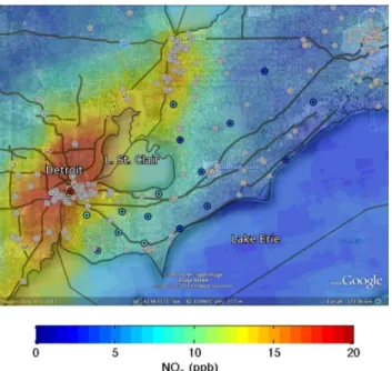
Fig. 8. Map of the campaign area with passive monitoring site
campaign averages and emissions sources. Colour indicates OMI-inferred NO2. The passive sites are marked by coloured circles with
the colour of the circle representing the campaign average NO2 con-centration (same colour scale as map). US EPA emissions sources with 2005 emissions greater than 100 t NOx/yr are marked on the
US side, while Environment Canada NPRI emissions greater than 100 t NO2/yr are marked.
OMI-inferred NO2 concentrations also follows the
distri-bution of emissions sources with many of the NO2 point
sources, as reported by the Environment Canada National Pollutant Release Inventory and the United States Environ-mental Protection Agency. Figure 8 shows that many sources are clustered around the Detroit-Windsor urban area and along the border between Lake St. Clair and Lake Huron.
The procedure for calculating surface NO2 from OMI
columns was performed in two ways: once using the campaign-only NO2data in addition to the permanent MoE
monitoring sites (7 sites total), and once using only the permanent MoE monitoring sites (5 sites). Correlation be-tween OMI measurements and passive measurements im-proved from 0.52 using raw OMI NO2columns to 0.69, with
a slope of 1.18, using the OMI inferred surface concentra-tions (Fig. 9). Interestingly, when only the MoE permanent monitoring stations were used, a correlation of 0.66 was ob-tained, but the slope increased from 1.18 to 1.32. The higher slope obtained when using only the five permanent MoE sites is attributed to their locations near NOx sources in urban
sites. These in-situ NO2 measurement are expected to be
less representative of the overall pixel area whose average column is measured by OMI.
The surface-to-column ratios used to calculate OMI-inferred surface-level NO2 concentrations varied somewhat
0 5 10 15 20 25
0 5 10 15 20 25
R = 0.69 slope = 1.18
Passive NO
2 (ppb)
OMI Inferred NO
2
(ppb)
Fig. 9. Passive measurements taken during the BAQS-met
cam-paign over 7 sampling periods at 17 simultaneous locations versus OMI inferred NO2concentrations at those same locations for the same periods.
across the 7 CL monitor sites with the lowest average ratio being 0.36 ppb/1×1015molec cm−2(i.e., 8.6×10⁻⁶cm−1) at the Environment Canada Bear Creek site and the max-imum average ratio being 1.66 ppb/1×1015molec cm−2 (4.0×10⁻⁵cm−1) at the MoE Chatham site. It is worth noting that the inverse of these surface-to-column ratios rep-resents a characteristic height (H) that varied from 250 to 1160 m. This metric provides a measure of the vertical ex-tent of the NO2, assuming that the ground based
measure-ment was representative of the OMI pixel.
In the case of the MoE Chatham site, the most likely lo-cal emission source is on-road vehicles. The urban area of Chatham itself is small (∼5 km in diameter or 20 km2) and surrounded by rural areas. Thus, the surface NO2
con-centration within Chatham tends to be higher than that in the surrounding rural region. As a result, measurement at this MoE site is less representative of the area over which the OMI measurements are averaged, which is a minimum of 300 km2. Since most of the area included in the OMI pixel footprint is the surrounding rural area, as opposed to the urban area of Chatham, the high in situ concentration in Chatham and the low overall column density would result in a high surface-to-column ratio, as observed.
In the region upwind of the Bear Creek site there are a number of stack emissions sources (Fig. 8). Thus, NO2in
this rural region has a higher potential to be above ground, compared to the vehicle emissions in Chatham. The low surface-to-column ratio determined for this site reflects this situation. The hypothesis of lofted NO2in this rural area is
also borne out by the inferred NO2at the location of the
Table 3. Mean surface-to-column ratio (±95 % confidence interval) and characteristic height, by season.
Season Mean surface-to-column ratio Mean characteristic (±95 % CI) (ppb/1×1015molec cm−2) height (m)
Winter 2.0 (±0.41) 210
Spring 1.7 (±0.13) 245
Summer 0.94 (±0.07) 450
Autumn 0.81 (±0.07) 525
5.4 ppb higher, on average, than the concentrations measured by this passive monitor.
These two extreme situations highlight some of the lim-itations of this approach. Using a CTM to provide a bet-ter estimate of the free-tropospheric column and applying Eq. (4) of Lamsal et al. (2008) could potentially lead to im-provements in the surface NO2estimates, especially in rural
areas. Another possible approach would be to empirically determine a spatially varying surface-to-column ratio, by fit-ting a polynomial surface to interpolate the measured point values. However, for this approach to work, a higher den-sity in situ monitoring network would be required to capture the variability and to account for the uncertainty in each in-dividual surface-to-column measurement. The simplest step towards improving the inference of ground-based NO2from
OMI data would be to increase the proportion of NO2
moni-toring locations at rural sites.
3.3.2 Temporal patterns
Temporal patterns in the OMI data and inferred ground-based concentrations were explored to illustrate the appli-cation of this methodology. The patterns examined in-cluded the variation in inferred concentrations across the region over four years, and the seasonality in the surface-to-column ratio. Over a span of 4 yr, using only the 5 permanent MoE monitoring stations, the seasonal average surface-to-column ratio was found to vary from a mini-mum of 0.81 ppb/1×1015molec cm−2 (H=525 m) in the autumn and a maximum of 2.0 ppb/1×1015molec cm−2 (H=210 m) in the winter (Table 3). No significant rela-tionship with characteristic height was found for any mete-orological variable. However, Lake Erie’s water temperature normally follows a very similar seasonal trend, with winter and spring (December through May) having lower lake tem-peratures than summer and autumn (June through Novem-ber) (NOAA, 2010). Therefore, it appears that higher lake temperatures in the summer and autumn may be driving the vertical mixing of NO2in the region, as seen in the seasonal
pattern in characteristic height.
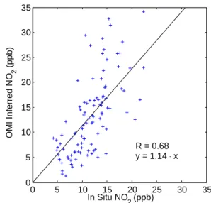
In order to verify the validity of the surface NO2procedure
developed from the BAQS-Met period for use over longer time spans, we calculated two week average OMI-derived
0 5 10 15 20 25 30 35
0 5 10 15 20 25 30 35
R = 0.68
y = 1.14 ⋅ x
In Situ NO
2 (ppb)
OMI Inferred NO
2
(ppb)
Fig. 10. Two-week average OMI inferred surface NO2vs. in situ
CL NO2measurements for 2005–2009. Improvement in correlation
(R=0.61 for DOMINO columns vs. in situ) was mainly due to a few periods in winter months, which showed greater agreement after the inference method was applied.
surface-level NO2concentrations using only 4 of the 5
avail-able permanent MoE monitoring sites, retaining the last site for evaluation. For this purpose, two week averages were cal-culated for both in situ CL measured NO2concentration at
the hold-back site and OMI-inferred NO2concentration for
the nearest 0.1◦grid cell. This procedure was done for every 2-week period from January 2005 to December 2009, ran-domly changing which site was held back each time. Surface inferred OMI concentrations showed a stronger correlation (R=0.68, Fig. 10) with in-situ CL-measured 2-week aver-ages than OMI column values (R=0.61). This provides con-fidence that the inference method is applicable to other peri-ods (i.e., not just the summer 2007 BAQS-met campaign pe-riod), continuing to add skill to the estimates of surface NO2.
This improvement (i.e. increase in correlation) is largely due to a few specific periods which appear to benefit the most from the inference method. These periods all occurred be-tween the months of November and March, and were ob-served across all 5 yr. These months tend to have more pixels excluded due to clouds and snow. Column averages calcu-lated from fewer overpasses would suffer more from day-to-day variations in the surface-to-column ratio, whereas our method removes this influence from each overpass. Further-more, OMI NO2 retrievals are expected to be biased over
snow (O’Byrne et al., 2010); our approach empirically cor-rects for that bias.
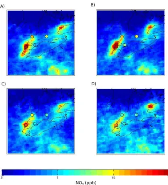
As an illustrative example, Fig. 11 provides regional snap-shots of OMI-inferred surface NO2concentrations for 4 yr.
From 2006 to 2009, OMI-inferred NO2 in the region
Fig. 11. OMI inferred NO2 concentrations for summers of (A) 2006, (B) 2007, (C) 2008 and (D) 2009. Colour circles
rep-resent average in situ measurements over the same time periods, on the same colour scale as the maps.
summer of 2009. This decrease in regional NO2
concen-trations may have coincided with a drop in manufacturing in the area during the economic slowdown after the fall of 2008. Concentrations over the West end of Lake Erie re-mained fairly stable in comparison with concentrations on-shore nearby, indicating that meteorologically driven disper-sion of NO2remained constant over 3 of the 4 yr in question.
3.3.3 Spatial patterns
Figure 12 shows average OMI inferred surface NO2
concen-trations for the entire 2007 year separated by wind direction. It is important to acknowledge the implicit assumption that exclusion of some days due to clouds does not introduce any bias in the maps. The long term comparison using the leave-one-out approach indicates that this is true, in general. It is possible, however, that, when separating overpasses by wind direction, we are exposing systematic errors which are masked by combining all overpasses. That is, if cloudy days from the southeast direction are cleaner than clear days and if cloudy days from the southwest direction are more polluted than clear days, by combining the days from both of these directions the errors cancel each other out. Also, it should be pointed out that the same single surface-to-column ratio calculated for the BAQS-met study area was applied across the entire range of the maps. The error introduced by this as-sumption may grow as the distance from the original points
Fig. 12. OMI inferred NO2 concentrations for 2007 grouped by
surface wind direction as measured at Windsor. (A) represents only OMI measurements taken when wind was blowing from the NW direction. (B, C and D) Same as (A) but NE, SW and SE directions, respectively. NW coast of Lake St. Clair indicated by black ar-row in (D); inferred concentrations over the lake are approximately half those onshore when the lake is upwind of the onshore emis-sions sources (i.e. when the wind blows from the SE). Number of overpasses used to generate each average was 21 (21 % of available overpasses) for (A), 70 for (B), 98 for (C) and 48 for (D). The total number of overpasses used is less than the total number of days in the year because of rejection of overpasses for which>2 surface stations were occluded by clouds.
of calculation grows and therefore what appear to be large differences between wind directions around the Toronto area (Northeast corner of the maps) could in fact be errors intro-duced by this assumption.
Figure 12d includes OMI measurements when the wind was blowing from due East to due South directions. This quadrant was particularly important to the study of the region because it illustrated the impact of easterly airflows nearly perpendicularly across the Canada-US border at Windsor-Detroit, thus highlighting any NOxemissions sources on the
Canadian side. The sharpness of the boundary can be ob-served on the NW shore of Lake St Clair (marked by a black arrow in Fig. 12d): over the lake the column measures ap-proximately half those immediately adjacent the lake on the NW shore.
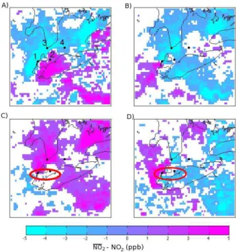
In order to more clearly see the effects of wind direc-tion on surface level NO2 concentrations, Fig. 13 shows
Fig. 13. Difference between OMI inferred NO2grouped by wind
direction and annual average OMI inferred NO2. Purple (positive), indicates higher than average NO2concentrations when the wind
blows from that direction while blue indicates lower than average concentrations. Uncoloured regions are less than 1 ppb difference. Labeled points in (A) represent surface monitoring stations (1: WW and WD; 2: CH; 3: SA; 4: LO) (A) represents only OMI measure-ments taken when wind was blowing from the NW direction. (B, C and D) Same as (A) but NE, SW and SE directions, respectively. See text for in-depth description regarding marked areas in (C) and (D).
wind directions). Overall, NO2concentrations were higher
when the wind blew from the SE and SW. Looking at the campaign area, the area between Lake Erie and Lake St. Clair (circled in red in Fig. 13c, d), a different pattern emerges: the area remains relatively unaffected by wind direction except for markedly elevated NO2 concentrations
across the entire region, as well as the west end of Lake Erie, when the wind blows from the NW. Good agreement between the satellite-derived, wind-direction-dependent con-centrations and in-situ, wind-direction-dependent concentra-tions was also found.
It should also be possible to discern areas of intense emis-sions from the difference maps. Indeed, the core of De-troit/Windsor, near the Ambassador Bridge over the Detroit River, is consistently found to be a boundary between be-low average and above average concentrations, for all wind directions (Fig. 13). Another area of interest is the area to the north of Lake St. Clair, just south of Sarnia where a large power generation station is situated in Ontario, as well as sev-eral emissions sources on the US side. Outflow can be seen from Cleveland, on the south side of Lake Erie, especially over the lake when wind flows from the SW.
4 Conclusions
We have shown that utilization of empirically calculated surface-to-column ratios in conjunction with OMI satel-lite NO2 column measurements can provide reasonable
long-term surface concentrations at a regional-to-local scale (∼11 km resolution). The approach leads to useful infor-mation on spatial and temporal variations in surface NO2,
if sufficient in situ measurements (average monitor spacing
<100 km) are available for the region. This approach has the advantage of providing an empirical correction for the bias in OMI NO2retrievals.
We showed that this method can be exploited to examine the extent of outflow of urban air pollution at a regional scale. Significant contributions to rural NO2 pollution in
South-western Ontario were displayed when wind flowed from the NW direction, due to outflow from the Windsor-Detroit area. These examples have shown how future work using these types of maps in qualitative and quantitative analyses such as population exposure assessment and model evaluation, could be conducted.
NOzinterference was quantified using collocated monitors
and it was shown that intake line adsorption and desorption contribute to both the magnitude of this interference and its temporal smoothing. Because of this smoothing, the effects of high midday ratios of(NO2)m/NO2, driven largely by low
midday NO2 values, can be mitigated by using whole-day
averages.
It should be noted that, although the long term results were calculated using only the urban monitoring stations per-manently maintained by the Ontario Ministry of the Envi-ronment, comparison of OMI inferred NO2 concentrations
to campaign passive monitoring data showed a slope much closer to one when rural monitoring locations were also in-cluded. This was attributed mainly to the situation of per-manent monitoring stations near sources, making these point sources less representative of the entire spatial footprint rep-resented by a single OMI pixel measurement of the same lo-cation. It may be sensible, therefore, in future to allocate more monitoring resources to rural areas, where spatial dis-tribution of NO2is less heterogeneous, to aid in
interpreta-tion of satellite results, which can yield significant insights into regional scale air quality.
Acknowledgements. We would like to thank the Canadian Foun-dation for Climate and Atmospheric Sciences for funding for this study and the Ontario Ministry of the Environment for providing NO2 data and support for the BAQS-met campaign, and Sandy Benetti for conducting the passive sampling field work and IC analysis.
References
Arain, M. A., Blair, R., Finkelstein, N., Brook, J., and Jerrett, B.: Meteorological influences on the spatial and temporal variability of NO2in Toronto and Hamilton, Can. Geogr.-Geogr. Can., 53,
165–190, 2009.
Boersma, K., Eskes, H., and Brinksma, E.: Error analysis for tropo-spheric NO2retrieval from space, J. Geophys. Res.-Atmos., 109,
D04311, doi:10.1029/2003JD003962, 2004.
Boersma, K. F., Eskes, H. J., Veefkind, J. P., Brinksma, E. J., van der A, R. J., Sneep, M., van den Oord, G. H. J., Levelt, P. F., Stammes, P., Gleason, J. F., and Bucsela, E. J.: Near-real time retrieval of tropospheric NO2from OMI, Atmos. Chem. Phys.,
7, 2103–2118, doi:10.5194/acp-7-2103-2007, 2007.
Boersma, K. F., Jacob, D. J., Bucsela, E. J., Perring, A. E., Dirksen, R., van der A, R. J., Yantosca, R. M., Park, R. J., Wenig, M. O., Bertram, T. H., and Cohen, R. C.: Valida-tion of OMI tropospheric NO2 observations during INTEX-B and application to constrain NOx emissions over the Eastern
United States and Mexico, Atmos. Environ., 42, 4480–4497, doi:10.1016/j.atmosenv.2008.02.004, 2008.
Boersma, K. F., Jacob, D. J., Trainic, M., Rudich, Y., DeSmedt, I., Dirksen, R., and Eskes, H. J.: Validation of urban NO2
concen-trations and their diurnal and seasonal variations observed from the SCIAMACHY and OMI sensors using in situ surface mea-surements in Israeli cities, Atmos. Chem. Phys., 9, 3867–3879, doi:10.5194/acp-9-3867-2009, 2009.
Bovensmann, H., Burrows, J. P., Buchwitz, M., Frerick, J., Noel, S., Rozanov, V. V., Chance, K., and Goede, A. P. H.: SCIAMACHY: mission objectives and measurement modes, J. Atmos. Sci., 56, 127–150, 1999.
Brook, J. R., Burnett, R. T., Dann, T. F., Cakmak, S., Gold-berg, M. S., Fan, X., and Wheeler, A. J.: Further interpreta-tion of the acute effect of nitrogen dioxide observed in Cana-dian time-series studies, J. Expo. Sci. Env. Epid., 17, S36–S44, doi:10.1038/sj.jes.7500626, 2007.
Bucsela, E., Celarier, E., Wenig, M., Gleason, J., Veefkind, J., Boersma, K., and Brinksma, E.: Algorithm for NO2
ver-tical column retrieval from the Ozone Monitoring In-strument, IEEE T. Geosci. Remote, 44, 1245–1258, doi:10.1109/TGRS.2005.863715, 2006.
Bucsela, E. J., Perring, A. E., Cohen, R. C., Boersma, K. F., Celarier, E. A., Gleason, J. F., Wenig, M. O., Bertram, T. H., Wooldridge, P. J., Dirksen, R., and Veefkind, J. P.: Compari-son of tropospheric NO2from in situ aircraft measurements with near-real-time and standard product data from OMI, J. Geophys. Res.-Atmos., 113, D16S31, doi:10.1029/2007JD008838, 2008. Burrows, J., Weber, M., Buchwitz, M., Rozanov, V.,
Ladstatter-Weissenmayer, A., Richter, A., DeBeek, R., Hoogen, R., Bram-steadt, K., Eichmann, K., Eisinger, M., and Perner, D.: The Global Ozone Monitoring Experiment (GOME): mission con-cept and first scientific results, J. Atmos. Sci., 56, 151–175, 1999. Celarier, E. A., Brinksma, E. J., Gleason, J. F., Veefkind, J. P., Cede, A., Herman, J. R., Ionov, D., Goutail, F., Pommereau, J. P., Lambert, J. C., van Roozendael, M., Pinardi, G., Wittrock, F., Sch¨onhardt, A., Richter, A., Ibrahim, O. W., Wagner, T., Bo-jkov, B., Mount, G., Spinei, E., Chen, C. M., Pongetti, T. J., Sander, S. P., Bucsela, E. J., Wenig, M. O., Swart, D. P. J., Volten, H., Kroon, M., and Levelt, P. F.: Validation of Ozone Monitoring Instrument nitrogen dioxide columns, J. Geophys.
Res., 113, D15S15, doi:10.1029/2007JD008908, 2008. Clark, N. A., Demers, P. A., Karr, C. J., Koehoorn, M., Lencar, C.,
Tamburic, L., and Brauer, M.: Effect of early life exposure to air pollution on development of childhood asthma, Environ. Health Persp., 118, 284–290, doi:10.1289/ehp.0900916, 2010. Hains, J. C., Boersma, K. F., Kroon, M., Dirksen, R. J.,
Cohen, R. C., Perring, A. E., Bucsela, E., Volten, H., Swart, D. P. J., Richter, A., Wittrock, F., Sch¨onhardt, A., Wag-ner, T., Ibrahim, O. W., van Roozendael, M., Pinardi, G., Glea-son, J. F., Veefkind, J. P., and Levelt, P.: Testing and improv-ing OMI DOMINO tropospheric NO2using observations from
the DANDELIONS and INTEX-B validation campaigns, J. Geo-phys. Res.-Atmos., 115, D05301, doi:10.1029/2009JD012399, 2010.
Halla, J. D., Wagner, T., Beirle, S., Brook, J. R., Hayden, K. L., O’Brien, J. M., Ng, A., Majonis, D., Wenig, M. O., and McLaren, R.: Determination of tropospheric vertical columns of NO2 and aerosol optical properties in a rural setting using
MAX-DOAS, Atmos. Chem. Phys. Discuss., 11, 13035–13097, doi:10.5194/acpd-11-13035-2011, 2011.
Herron-Thorpe, F. L., Lamb, B. K., Mount, G. H., and Vaughan, J. K.: Evaluation of a regional air quality forecast model for tropospheric NO2columns using the OMI/Aura
satel-lite tropospheric NO2product, Atmos. Chem. Phys., 10, 8839–
8854, doi:10.5194/acp-10-8839-2010, 2010.
Jerrett, M., Finkelstein, M. M., Brook, J. R., Arain, M. A., Kanaroglou, P., Stieb, D. M., Gilbert, N. L., Verma, D., Finkelstein, N., Chapman, K. R., and Sears, M. R.: A co-hort study of traffic-related air pollution and mortality in Toronto, Ontario, Canada, Environ. Health Persp., 117, 772–777, doi:10.1289/ehp.11533, 2009.
Kim, S. W., Heckel, A., Frost, G. J., Richter, A., Gleason, J., Bur-rows, J. P., McKeen, S., Hsie, E. Y., Granier, C., and Trainer, M.: NO2columns in the Western United States observed from space
and simulated by a regional chemistry model and their impli-cations for NOx emissions, J. Geophys. Res., 114, D11301,
doi:10.1029/2008JD011343, 2009.
Kramer, L. J., Leigh, R. J., Remedios, J. J., and Monks, P. S.: Comparison of OMI and ground-based in situ and MAX-DOAS measurements of tropospheric nitrogen dioxide in an urban area, J. Geophys. Res.-Atmos., 113, D16S39, doi:10.1029/2007JD009168, 2008.
Lamsal, L. N., Martin, R. V., van Donkelaar, A., Steinbacher, M., Celarier, E. A., Bucsela, E., Dunlea, E. J., and Pinto, J. P.: Ground-level nitrogen dioxide concentrations inferred from the satellite-borne Ozone Monitoring Instrument, J. Geophys. Res.-Atmos., 113, D16308, doi:10.1029/2007JD009235, 2008. Lamsal, L. N., Martin, R. V., van Donkelaar, A.,
Celar-ier, E. A., Bucsela, E. J., Boersma, K. F., Dirksen, R., Luo, C., and Wang, Y.: Indirect validation of tropospheric ni-trogen dioxide retrieved from the OMI satellite instrument: in-sight into the seasonal variation of nitrogen oxides at north-ern midlatitudes, J. Geophys. Res.-Atmos., 115, D05302, doi:10.1029/2009JD013351, 2010.
Lenters, V., Uiterwaal, C. S., Beelen, R., Bots, M. L., Fischer, P., Brunekreef, B., and Hoek, G.: Long-term exposure to air pol-lution and vascular damage in young adults, Epidemiology, 21, 512–520, doi:10.1097/EDE.0b013e3181dec3a7, 2010.
de Vries, J., Stammes, P., Lundell, J., and Saari, H.: The Ozone Monitoring Instrument, IEEE T. Geosci. Remote, 44, 1093– 1101, doi:10.1109/TGRS.2006.872333, 2006.
Levy, I., Makar, P. A., Sills, D., Zhang, J., Hayden, K. L., Mi-hele, C., Narayan, J., Moran, M. D., Sjostedt, S., and Brook, J.: Unraveling the complex local-scale flows influencing ozone pat-terns in the southern Great Lakes of North America, Atmos. Chem. Phys., 10, 10895–10915, doi:10.5194/acp-10-10895-2010, 2010.
Makar, P. A., Gong, W., Mooney, C., Zhang, J., Davignon, D., Samaali, M., Moran, M. D., He, H., Tarasick, D. W., Sills, D., and Chen, J.: Dynamic adjustment of climatological ozone bound-ary conditions for air-quality forecasts, Atmos. Chem. Phys., 10, 8997–9015, doi:10.5194/acp-10-8997-2010, 2010.
Martin, R. V., Chance, K., Jacob, D. J., Kurosu, T. P., Spurr, R. J. D., Bucsela, E., Gleason, J. F., Palmer, P. I., Bey, I., Fiore, A. M., Li, Q., Yantosca, R. M., and Koelemeijer, R. B. A.: An improved retrieval of tropospheric nitrogen dioxide from GOME, J. Geo-phys. Res., 107, 4437, doi:10.1029/2001JD001027, 2002. MoE: Air Quality in Ontario 2008 Report, available at: http://
www.ene.gov.on.ca/publications/7356e.pdf (last access: August 2010), 2008.
NOAA: Lake Erie Temperature Normals, available at: http://www. erh.noaa.gov/buf/laketemps/lktemp.html (last access: December 2010), 2010.
O’Byrne, G., Martin, R. V., van Donkelaar, A., Joiner, J., and Celarier, E. A.: Surface reflectivity from the Ozone Monitor-ing Instrument usMonitor-ing the Moderate Resolution ImagMonitor-ing Spectro-radiometer to eliminate clouds: effects of snow on ultraviolet and visible trace gas retrievals, J. Geophys. Res., 115, D17305, doi:10.1029/2009JD013079, 2010.
Ord´o˜nez, C., Richter, A., Steinbacher, M., Zellweger, C., Nuss, H., Burrows, J., and Prevot, A.: Comparison of 7 years of satellite-borne and ground-based tropospheric NO2
measure-ments around Milan, Italy, J. Geophys. Res.-Atmos., 111, D05310, doi:10.1029/2005JD006305, 2006.
Russell, A. R., Valin, L. C., Bucsela, E. J., Wenig, M. O., and Co-hen, R. C.: Space-based constraints on spatial and temporal pat-terns of NOxemissions in California, 2005–2008, Environ. Sci.
Technol., 44, 3608–3615, doi:10.1021/es903451j, 2010. Ryerson, T., Williams, E., and Fehsenfeld, F.: An e?cient photolysis
system for fast-response NO2measurements, J. Geophys.
Res.-Atmos., 105, 26447–26461, 2000.
Statistics Canada: 2006 Census of Canada Census Profiles Marital status, common-law status, families, dwellings, and households Tables: Profile of Marital Status, Common-law Status, Fami-lies, Dwellings and Households, for Census Metropolitan Areas and Census Agglomerations, 2006 Census., Tech. rep., Statistics Canada, 2006.
Steinbacher, M., Zellweger, C., Schwarzenbach, B., Bugmann, S., Buchmann, B., Ordonez, C., Prevot, A. S. H., and Hueglin, C.: Nitrogen oxide measurements at rural sites in Switzerland: Bias of conventional measurement techniques, J. Geophys. Res.-Atmos., 112, D11307, doi:10.1029/2006JD007971, 2007. US Census Bureau: Table 1. Annual Estimates of the
Popula-tion of Metropolitan and Micropolitan Statistical Areas: 1 April 2000 to 1 July 2009 (CBSA-EST2009-01), available at: http:// www.census.gov/popest/metro/CBSA-est2009-annual.html (last access: October 2010), 2010.
Wenig, M., Cede, A., Bucsela, E., Celarier, E., Boersma, K., Veefkind, J., Brinksma, E., Gleason, J., and Herman, J.: Validation of OMI tropospheric NO2 column densities us-ing direct-Sun mode Brewer measurements at NASA Goddard Space Flight Center, J. Geophys. Res.-Atmos., 113, D16S45, doi:10.1029/2007JD008988, 2008.