A multi-year methane inversion using SCIAMACHY, accounting for systematic errors using TCCON measurements

(1)

Atmos. Chem. Phys., 14, 3991–4012, 2014 www.atmos-chem-phys.net/14/3991/2014/ doi:10.5194/acp-14-3991-2014

Atmospheric

Chemistry

and Physics

A multi-year methane inversion using SCIAMACHY, accounting for

systematic errors using TCCON measurements

S. Houweling1,2, M. Krol1,2,3, P. Bergamaschi4, C. Frankenberg5, E. J. Dlugokencky6, I. Morino7, J. Notholt8,

V. Sherlock9, D. Wunch10, V. Beck11, C. Gerbig11, H. Chen12,13, E. A. Kort14, T. Röckmann2, and I. Aben1

1_{SRON Netherlands Institute for Space Research, Utrecht, the Netherlands}

2_{Institute for Marine and Atmospheric Research (IMAU), Utrecht University, Utrecht, the Netherlands} 3_{Department of Meteorology and Air Quality (MAQ), Wageningen University and Research Centre,}

Wageningen, the Netherlands

4_{European Commission Joint Research Centre, Institute for Environment and Sustainability, Ispra (Va), Italy} 5_{Jet Propulsion Laboratory, Pasadena, CA, USA}

6_{NOAA Earth System Research Laboratory, Global Monitoring Division, Boulder, CO, USA}

7_{Center for Global Environmental Research, National Institute for Environmental Studies (NIES) Onogawa 16-2, Tsukuba,}

Ibaraki 305-8506, Japan

8_{Institute of Environmental Physics, University of Bremen, Bremen, Germany}

9_{National Institute of Water and Atmospheric Research (NIWA), P.O. Box 14-901, Wellington, New Zealand} 10_{Caltech, Pasadena, CA, USA}

11_{Max Planck Institute for Biogeochemistry, Jena, Germany}

12_{Center for Isotope Research (CIO), University of Groningen, the Netherlands} 13_{CIRES, University of Colorado, Boulder, CO, USA}

14_{Department of Atmospheric, Oceanic and Space Sciences, University of Michigan, Ann Arbor, MI, USA} Correspondence to:S. Houweling (s.houweling@sron.nl)

Received: 21 August 2013 – Published in Atmos. Chem. Phys. Discuss.: 30 October 2013 Revised: 2 March 2014 – Accepted: 7 March 2014 – Published: 22 April 2014

Abstract. This study investigates the use of total column

CH4(XCH4) retrievals from the SCIAMACHY satellite

in-strument for quantifying large-scale emissions of methane. A unique data set from SCIAMACHY is available span-ning almost a decade of measurements, covering a period when the global CH4growth rate showed a marked transition

from stable to increasing mixing ratios. The TM5 4DVAR in-verse modelling system has been used to infer CH4emissions

from a combination of satellite and surface measurements for the period 2003–2010. In contrast to earlier inverse mod-elling studies, the SCIAMACHY retrievals have been cor-rected for systematic errors using the TCCON network of ground-based Fourier transform spectrometers. The aim is to further investigate the role of bias correction of satellite data in inversions. Methods for bias correction are discussed, and the sensitivity of the optimized emissions to alternative bias correction functions is quantified. It is found that the use of

SCIAMACHY retrievals in TM5 4DVAR increases the esti-mated inter-annual variability of large-scale fluxes by 22 % compared with the use of only surface observations. The dif-ference in global methane emissions between 2-year periods before and after July 2006 is estimated at 27–35 Tg yr−1_{. The}

use of SCIAMACHY retrievals causes a shift in the emis-sions from the extra-tropics to the tropics of 50±_{25 Tg yr}−1_.

(2)

1 Introduction

To reduce the uncertainty of climate change prediction, im-proved understanding of the global cycles of long-lived greenhouse gases is needed. This is true in particular for methane, the second most important anthropogenic green-house gas, which has shown important growth rate variations in the past 2 decades that are only poorly understood (Dlu-gokencky et al., 2009; Kirschke et al., 2013; Aydin et al., 2011; Pison et al., 2013). To study the drivers of changes in the methane growth rate requires tools for quantifying its sources and sinks at large scales, which remains a scientifi-cally challenging task.

Inverse modelling techniques make use of independent in-formation from atmospheric measurements, to improve the available emission estimates and to reduce their uncertain-ties. In the past, these techniques have most commonly been applied to ground-based measurements from global monitor-ing networks (Bousquet et al., 2006, 2011; Houwelmonitor-ing et al., 1999; Hein et al., 1997). In recent years, measurements from satellites have become available, such as from SCIAMACHY (Bovensmann et al., 1999; Frankenberg et al., 2005, 2008a, 2011; Schneising et al., 2011) and more recently also from GOSAT (Yokota et al., 2009; Kuze et al., 2009; Butz et al., 2011; Schepers et al., 2012), and significant efforts have been spent to investigate their use in inverse modelling (Meirink et al., 2008a; Bergamaschi et al., 2009, 2013; Fraser et al., 2012).

Satellite instruments offer spectacular improvements in measurement coverage, particularly over tropical continents, which have been the Achilles heel of the surface monitoring networks for many years. Using satellite retrievals, several studies have addressed the size of the tropical methane flux, pointing to previously underestimated emissions (Franken-berg et al., 2005, 2008a; Bergamaschi et al., 2009; Beck et al., 2012; Bergamaschi et al., 2013) that were corrected down-ward in part after revisions of the methane and water vapour spectroscopy (Frankenberg et al., 2008a, b). Despite these efforts, however, inversion-derived tropical methane emis-sions remain highly uncertain due to the methodological dif-ficulty of accounting for poorly characterized measurement and transport model uncertainties.

The use of SCIAMACHY retrievals in inverse modelling requires a bias correction algorithm (Bergamaschi et al., 2009, 2013). The common approach is to account for incon-sistencies between surface and satellite measurements using a set of bias correction functions that are optimized along with the methane sources and sinks. Here, surface measure-ments are used in addition to the satellite data to provide ad-ditional constraints on the surface fluxes and act as anchor points to constrain the parameters of the bias correction func-tions. However, it is not clear how to best define the bias correction functions and to account for their uncertainties. The problem is further complicated by transport model un-certainties and model–data representation errors, which have

systematic error components also. The approach taken by Meirink et al. (2008b) and Bergamaschi et al. (2013) is to optimize a quadratic function of latitude for each month of available data, to account for inconsistencies between mod-elled and observed latitudinal and seasonal variations in the total column-averaged methane mixing ratio (XCH4).

For inverse modelling applications spanning many years of data this approach has two important limitations. First, since the bias functions have no direct relationship with known shortcomings of the measurements, it is unclear to which extent the optimized parameters account for system-atic error in the measurements, or systemsystem-atic model error, or real signals in the satellite data. Secondly, the number of bias parameters increases proportionally with the number of years, introducing additional degrees of freedom capable of absorbing much of the information on inter-annual variation provided by the measurements.

The purpose of this study is to further investigate the role of measurement bias in methane inversions using satellite data, to assess how sensitive studies such as Bergamaschi et al. (2013) are to the bias correction method that is used. For this purpose, an alternative approach to bias correction is introduced, which makes use of measurements from the To-tal Carbon Column Observing Network (TCCON) (Wunch et al., 2011a) to identify systematic errors in satellite re-trievals. Several versions are tested to study the sensitivity of the optimized fluxes to the bias correction method, includ-ing a direct comparison with results from Bergamaschi et al. (2013). Further, we test whether comparisons with indepen-dent measurements allow evaluation of the bias correction approach.

Inverse modelling calculations are carried out using TM5 4DVAR (Meirink et al., 2008b; Bergamaschi et al., 2013) for the period 2003–2010, with and without the use of SCIA-MACHY retrievals (Frankenberg et al., 2011). This period covers the transition from stationary to increasing methane mixing ratios, and therefore allows us to contribute to the ongoing discussion about the underlying causes. Optimized fluxes derived using only surface measurements act as a ref-erence for assessing the contribution from SCIAMACHY in joint inversions of surface and satellite data.

(3)

4

2 Methods

2.1 TM5 4DVAR

The TM5 4DVAR inverse modelling system has been used in studies of several atmospheric trace gases, including CH4

(Meirink et al., 2008b; Bergamaschi et al., 2009, 2010), CO (Hooghiemstra et al., 2012a, b), CO2 (Basu et al., 2013;

Guerlet et al., 2013) and CH3CCl3 (Montzka et al., 2011).

Here it is used for estimating large-scale emissions of CH4,

by optimizing the agreement between measured and model simulated mixing ratios. This is achieved by minimizing a Bayesian cost functionJ(x), defined as

J(x)=1

2((y−Hx)

T_R−1₍_y₋_H_x₎₊₍_x₋_x

0)TB−1(x₋x0)), (1)

with respect to a state vector of surface fluxesx.His a

Ja-cobian matrix of the sensitivity of the observed mixing ra-tios to the surface fluxes, calculated using the atmospheric transport model TM5 (Krol et al., 2005). The misfits to the measurementsyand a priori fluxesx0are weighted by their

respective uncertainties (RandB).

Equation (1) is solved using the variational approach de-scribed by Meirink et al. (2008b). In short, an iterative proce-dure is followed of alternating forward and adjoint transport model simulations. The forward model is used to calculate model–data mismatches (y−Hx) for each successive update of the flux vectorx. The adjoint model (HT) uses the model– data mismatch vector to evaluate the cost function gradient (∇J(x)), represented by

∇J(x)=B−1(x−x0)−HTR−1(y−Hx). (2)

The trial state vectorxand corresponding cost function gra-dient are input to a Lanczos minimization algorithm (Lanc-zos, 1950), yielding an updated state vector. The procedure is terminated after a fixed number of iterations or after the re-maining gradient passes a preset convergence criterion. The inversion results presented in this article are obtained after 55 iterations, which corresponds to a gradient norm reduction of about a factor 5000.

TM5 simulations were performed for the period 2003–2010 using meteorological fields from the ECMWF ERA Interim reanalysis project (Dee et al., 2011), pre-processed for use in TM5 at 4◦_×₆◦ _(latitude_×_longitude)

and 25 hybrid sigma pressure levels from the surface to the top of the atmosphere. The inversion makes use of the “cy1” version of TM5-4DVAR, extended with a parametrization of horizontal diffusion using the modified version of Prather et al. (1987) described in Monteil et al. (2013). This scheme has been introduced to account for the underestimated inter-hemispheric mixing rate in TM5 reported in Patra et al. (2011). The tuning parameter for the horizontal diffusion strength (D in Prather et al., 1987) is adjusted such that the TM5 simulated north–south gradient

for the year 2003 is brought in agreement with available measurements of SF6(see Monteil et al., 2013).

The inversion solves for the monthly mean CH4flux into

each surface grid box of the model. Note that, in contrast to Bergamaschi et al. (2013), no distinction is made between contributions from different processes, because the measure-ments provide only limited process-specific information at the resolution of the transport model. Also, they provide lim-ited information to distinguish between surface fluxes and atmospheric sinks. For this reason we choose to solve for sur-face fluxes only, which are thus optimized given the assumed atmospheric sinks.

2.2 A priori fluxes

Anthropogenic emissions from fossil fuel use, agricul-tural practices and waste treatment are taken from the EDGAR4.1 emission inventory (European Commission, Joint Research Centre (JRC)/Netherlands Environmental As-sessment Agency (PBL), 2010), which provides annual emis-sions at 0.1◦_×_0.1◦_{resolution until the end of 2005. For the}

period 2005–2010 we extrapolate the EDGAR4.1 emission maps of 2005 using global statistics made available by BP (statistical review of world energy 2011, http://www.bp.com) and FAO (FAOSTAT, see http://faostat.fao.org). For fossil fuel use, we scale the gridded EDGAR4.1 emissions for 2005 by the fractional increase of global fuel production and con-sumption since 2005. Our extrapolation procedure differen-tiates between different fuel types (oil, coal and gas), and sources classified as “energy production”. For the remain-ing fossil sources, such as the EDGAR category “residential commercial and others”, we choose the BP reported produc-tion/consumption categories that best reproduce the EDGAR emissions for the period until 2005.

For agricultural sources, we apply the same procedure using FAO reported indices for gross production, rice pro-duction and cattle number. Remaining categories, for ex-ample waste treatment, are extrapolated using a linear re-gression of the global EDGAR4.1 emissions for the period 2000–2005. This procedure yields an increase of anthro-pogenic CH4 emissions between the years 2003 and 2010

of 37 Tg CH4yr−1. EDGAR4.1 does not provide

informa-tion on intra-annual emission variainforma-tions. In TM5 we neglect seasonal variations in fossil and agricultural sources, except emissions from rice agriculture, which are distributed sea-sonally following the rice cropping calendar of Matthews and Fung (1987).

(4)

regions with rice agriculture, LPJ-WhyMe emissions are not used, to avoid double counting. Biomass burning emissions are taken from GFED3.1 (van der Werf et al., 2010), except for emissions from agricultural waste burning, which are in-cluded in EDGAR4.1.

Geologic sources of methane have received much atten-tion in recent years (Etiope and Klusman, 2002; Etiope and Milkov, 2004; Kvenvolden and Rogers, 2005), with reported global emissions ranging between 13 and 80 Tg CH4yr−1

(Judd, 2004; Etiope et al., 2008). Their representation in global models is complicated by the limited number of mud volcanoes for which the emissions have been quantified. The available estimates vary widely and represent only a small fraction of the extrapolated global totals. Digital global maps that would be needed to construct gridded global emissions for use in models do not exist or are not made available for commercial reasons. This is true in particular for mi-cro seepage from sedimentary basins on land, with an es-timated global contribution exceeding 10 Tg CH4yr−1 and

covering 10 % of the global drylands (Etiope and Klusman, 2010). For this reason, we account only for 1300 mud volca-noes and seeps that are reported worldwide and are archived in the GLOGOS database (http://www.searchanddiscovery. com/documents/2009/090806etiope/). To avoid biasing our emissions to extensively studied sites, we distributed them evenly over all reported coordinates.

For marine seepage, the situation is similar. Despite coor-dinated activities to archive all available information (Bange et al., 2009), no global inventory is available yet. Our ap-proach is to distribute a conservative estimate of global emis-sions from marine seeps and hydrates of 17 Tg yr−1

uni-formly over the continental shelves (see Table 1). This sim-plified approach does not account for what is known from ongoing regional efforts to quantify, for example, the hot spot of geologic emissions in Azerbaijan (Etiope and Klus-man, 2002) or the reported marine seepages in the Laptev Sea (Shakhova et al., 2010). A priori flux uncertainties are set to 50 % of the combined monthly flux in each grid box of the model, with uniform and exponentially decaying spatial and temporal correlation scales amounting to, respectively, 1000 km and 3 months.

Tropospheric methane oxidation is represented using methyl chloroform optimized OH distributions (Huijnen et al., 2010). A single scaling factor of 0.92 is applied to the seasonal varying global OH field of Spivakovski et al. (2000), which is recycled each year of simulation, hence ignoring inter-annual variability. We do not account for the estimated contribution of marine Cl radicals to the tropospheric CH4

sink (Allan et al., 2001, 2005; Lassey et al., 2011). Strato-spheric CH4lifetimes are derived from the Cambridge 2-D

model (Law and Pyle, 1993), and account for CH4oxidation

by OH, O(1D), and Cl radicals.

Like most off-line transport models, TM5 tends to under-estimate the stratospheric age of air (Jones et al., 2001). To account for the generally overestimated contribution of upper

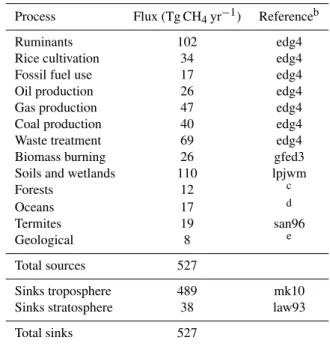
Table 1.A priori CH₄fluxes for the year 2005a.

Process Flux (Tg CH4yr−1) Referenceb

Ruminants 102 edg4

Rice cultivation 34 edg4

Fossil fuel use 17 edg4

Oil production 26 edg4

Gas production 47 edg4

Coal production 40 edg4

Waste treatment 69 edg4

Biomass burning 26 gfed3

Soils and wetlands 110 lpjwm

Forests 12 c

Oceans 17 d

Termites 19 san96

Geological 8 e

Total sources 527

Sinks troposphere 489 mk10

Sinks stratosphere 38 law93

Total sinks 527

a_{The numbers in this table correspond to what has been used as a priori}

information, but do not necessarily reflect the potential importance of each source. This is true in particular for geological sources (see text).

b_{edg4: European Commission, Joint Research Centre (JRC)/Netherlands}

Environmental Assessment Agency (PBL) (2010), gfed3: van der Werf et al. (2010), lpjwm: Spahni et al. (2011), san96: Sanderson (1996), mk10: Huijnen et al. (2010), law93: Law and Pyle (1993).

c_{Accounts for reported emissions from organic material (Vigano et al.,}

2008), tank bromeliads (Martinson et al., 2010) and other sources in upland tropical forests (Braga do Carmo et al., 2006).

d_{Includes emissions from open oceans (3 Tg CH}

4yr−1, Bates et al., 1996)

and continental shelves (14 Tg CH4yr−1, Kvenvolden and Rogers, 2005;

Etiope and Klusman, 2002).eEmissions from mud volcanoes, oil and gas seeps (GLOGOS database:

http://www.searchanddiscovery.com/documents/2009/090806etiope/).

stratospheric CH4toXCH4in TM5, we correct model

sam-pled vertical profiles above 50 hPa using a CH4climatology

based on HALOE/CLAES observations (Randel et al., 1998). This procedure includes a linear correction for the CH4

in-crease since the period of observation. Table 1 summarizes the prescribed a priori fluxes, including their corresponding global emissions for the year 2005.

2.3 Measurements

(5)

4

Extra Tropical NH

Tropics

Extra Tropical SH

Trop. S. America Trop. Africa S.E. Asia BRW ALT SHM ZEP BAL BSC CGO ICE PAL MLO SEY MID CHR RPB KEY BMW IZO ASK WLG BKT TAP GMI SPO ASC HUN SEY MHD AZR STM CRZ TDF UUM HBA SYO PSA WIS KUM

AMT KZM _KZD

UTA SGP LEF NWR PTA 1 2 4 3 5 6 7 8

Fig. 1.Location of NOAA and TCCON sites used in this study,

and of the regions used for integrating inversion-estimated fluxes. NOAA sites are indicated as yellow circles with corresponding site acronyms. The TCCON sites are indicated as blue circled numbers indicating 1: Park Falls, 2: Lamont, 3: Bialystok, 4: Garmisch, 5: Tsukuba, 6: Darwin, 7: Wollongong, 8: Lauder.

The data covariance matrix accounts for measurement un-certainties and model representation errors. We use the local concentration variability as a proxy for model representation error (also referred to as model data mismatch error). The as-signed value is the maximum of: (i) the standard deviation of the samples that are averaged, and (ii) the standard devi-ation of the simulated CH4mixing ratios in the surrounding

grid boxes. The measurement uncertainty is set to 2.4 ppb for surface measurements, which represents the average pair difference of the NOAA flask measurements. All errors are assumed independent.

We use SCIAMACHY retrievals from the IMAPv5.5 proxy retrieval reported by Frankenberg et al. (2011). The retrieved CH4/ CO2 ratios have been converted intoXCH4

using CarbonTracker-derived XCO2 (Peters et al., 2007).

Optimized CarbonTracker fields were unavailable for the last 3 years of our simulation. The CarbonTracker estimates for 2007 were extrapolated for those years using the global growth rate of CO2, estimated by averaging the surface

mea-surements from South Pole, Mauna Loa, and Alert. The use of SCIAMACHY retrievals is limited to 50◦_{N to 50}◦_S.

Representation errors for SCIAMACHY are calculated from the modelled local variability inXCH4, using the

sim-ulated columns in the surrounding grid boxes. For the mea-surement uncertainty we take the maximum of the retrieval uncertainty and the standard deviation of the averaged re-trievals. The spatio-temporal interval for averaging is the same as for the surface measurements. The uncertainties of the averaged SCIAMACHY retrievals are assumed to be un-correlated. To account for correlated retrieval error of nearby retrievals, we treat the errors of the retrievals within the 6◦_×₄◦_{grid boxes and 3-hourly intervals as fully correlated.}

This approach yields 1σ uncertainties in the range of 15 to 45 ppb. In addition, we account for measurement bias as de-scribed in the next section.

The SCIAMACHY bias correction, described in detail in the next section, makes use of TCCON data from the

GGG2012 release. Figure 1 shows the sites that were used. The estimated 1σ single measurement uncertainty for CH4,

after correction for systematic errors using aircraft profile measurements, amounts to 3.5 ppb (Wunch et al., 2010, 2011a).

2.4 Bias correction

A common approach to account for systematic measurement errors in inversions is to define a set of functions describ-ing the spatio-temporal dependence of these errors, with un-certain parameters that are optimized in the inversion along with the other elements of the state vector. Following this approach, the comparison between modelled and observed mixing ratios can be written as

yobs=Hxtrue+ǫ+

n X

i=0

fb(αi), (3)

whereǫandfb(αi)represent, respectively, the random and

systematic component of the data uncertainty. The system-atic error componentsfb(αi)are functions of the added state

vector elementsαi. As for the random errorǫ, the systematic

error has contributions from both the measurements and the model. In practice, well-quantified biases are usually directly corrected in the model or the measurements. Therefore, the bias correction we are dealing with here targets ill-defined residual biases. In our experience, the optimization of bias terms in the inversion can lead to solutions that are out of their a priori assigned uncertainty ranges. This is a sign that a bias function ends up accounting for other uncertain ele-ments in the inversion, such as unaccounted model errors or even the sources and sinks, which are meant to be estimated by the inversion. In that case, it may be preferable to pre-scribe the initial bias correction, without further optimiza-tion. In this study, we perform inversions with and without optimization of bias corrections to investigate the impact.

Different strategies can be followed for defining fb(αi),

using

1. empirical functions of space and time,

2. information about known retrieval uncertainties, 3. differences between retrievals and independent

mea-surements.

(6)

A good example is the study by Wunch et al. (2011b) on the use of TCCON data for evaluating systematic errors in ACOS-GOSATXCO2retrievals.

For SCIAMACHY XCH4, we constructed a model

of known retrieval uncertainties on the basis of Butz et al. (2010), accounting for spectroscopic errors varying with the sampled air mass and residual aerosol errors varying with the difference in surface albedo between the weak short-wave infra-red (SWIR) CO2 and CH4

absorption bands. Optimization of the bias coefficients in the inversion, however, turned out to be rather inefficient in correcting apparent inconsistencies in the optimized fits to surface and total column measurements (not shown). Analy-sis of the difference between co-located SCIAMACHY and TCCON measurements pointed to a seasonal pattern that correlates well with climatic variables such as temperature and humidity. These parameters lag variations in solar zenith angle (SZA), due to the inertia in the earth’s climate system, which may explain why the use of air mass for seasonal bias correction did not work well.

Figure 2 demonstrates the relation between the SCIA-MACHY seasonal bias with respect to TCCON and ERA-interim derived specific humidity. Vertical profiles of specific humidity are used that have also been used in the IMAP v5.5 retrieval. The values represent averages over the lowest 3 km of the vertical profile (up to∼_{700 hPa over sea). Influences}

of water vapour on the SCIAMACHY CH4 retrieval were

discussed by Frankenberg et al. (2008a), who corrected the water vapour spectroscopy in the 1.6 micron CH4

absorp-tion band. It is not clear whether water vapour is the cause of the seasonal bias discussed here, or that it only happens to covary with a different underlying cause. In either case, the correlation of the SCIAMACHY-TCCON residuals with water vapour offers a useful proxy for SCIAMACHY bias correction.

This finding motivated us to define a bias correction us-ing a limited set of functions accountus-ing for the main dif-ferences between SCIAMACHY and TCCON (i.e. a combi-nation of strategies 1 and 3). Besides seasonality, our bias correction method accounts for a global offset and a latitu-dinal correction. Note that the humidity proxy already intro-duces a latitudinal correction (as well as corrections on other timescales, including that of inter-annual variability). How-ever, differences with TCCON remain, which are corrected separately. Unfortunately, the TCCON network is not dense enough to derive a latitudinal correction function. To extend coverage, we make use of GOSAT proxy XCH4 retrievals

reported by Schepers et al. (2012), which are significantly more accurate than SCIAMACHY retrievals (see Schepers et al., 2012; Monteil et al., 2013). This is confirmed by Fig. 3, which shows that residuals between TCCON and seasonal-ity corrected SCIAMACHY show a similar latitudinal varia-tion as residuals between SCIAMACHY and GOSAT. To iso-late the large-scale component of this relationship, the

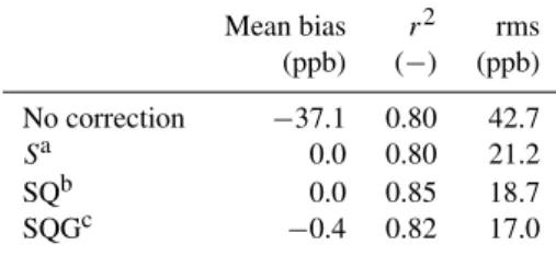
SCIA-Table 2. Statistics ofXCH₄residuals between TCCON and

bias-corrected SCIAMACHY retrievals.

Mean bias r2 rms

(ppb) (−) (ppb)

No correction −37.1 0.80 42.7

Sa 0.0 0.80 21.2

SQb 0.0 0.85 18.7

SQGc −0.4 0.82 17.0

a_{Uniform bias correction.} b_{Uniform + seasonal bias correction.}

c_{Uniform + seasonal + latitudinal bias correction.}

MACHY minus GOSAT residuals have been smoothed using a boxcar filter (width=20◦latitude).

In summary, the bias correction functions that we will in-vestigate are the following:

– S: a global uniform scaling factor only.

– SQ: as “S”, extended with the seasonal correction us-ing humidity.

– SQG: as “SQ”, extended with a latitudinal correction

using GOSAT.

The corresponding bias coefficientsαare determined by lin-ear regression to the SCIAMACHY–TCCON residuals, using TCCON measurements from the sites shown in Fig. 1 for the years 2009 and 2010. To obtain a single set of coefficients for use inS, SQ and SQG, the regressions were carried out in this order. Each extension was regressed to the TCCON– SCIAMACHY residuals up to that extension. To avoid in-terference withS, functionsQ andGwere normalized by

taking out their means.

Table 2 summarizes general statistics of the difference be-tween TCCON and co-located SCIAMACHY retrievals for the different stages of bias correction. As can be seen in Ta-ble 2, the uniform scaling factor decreases the rms differ-ence between TCCON and SCIAMACHY by about a factor of two. Smaller additional improvements are obtained after introducing the seasonal and latitudinal corrections. A large fraction of the remaining rms is explained by scatter in the retrievals on relatively small scales.

2.5 Experimental setup and scenarios

(7)

4

2009.5 2010.0 2010.5

time -40

-20 0 20 40

CH

4

(ppb)

-10 -5 0 5 10

q (g/kg)

Wollongong, Australia (151E, 34S) 2009.2 2009.4 2009.6 2009.8 2010.0 2010.2

time -40

-20 0 20 40

CH

4

(ppb)

-10 -5 0 5 10

q (g/kg)

Tsukuba, Japan (140E, 36N)

2009.5 2010.0 2010.5

time -40

-20 0 20 40

CH

4

(ppb)

-10 -5 0 5 10

q (g/kg)

Park Falls, U.S.A. (90W, 46N)

2009.5 2010.0 2010.5

time -40

-20 0 20 40

CH

4

(ppb)

-10 -5 0 5 10

q (g/kg)

Darwin, Australia (131E, 12S)

•

SCIAMACHY - TCCON XCH₄

•

ERA-Interim Speciic humidity

6

Fig. 2.Seasonal variation of residuals between co-located SCIAMACHY and TCCON measurements (black, leftyaxis) and its relation with

ERA-Interim derived specific humidity averaged between the surface and 3 km altitude (red, rightyaxis).

-40 -20 0 20 40

latitude (degree) -20

-10 0 10 20

6

XCH

4

(ppb)

Fig. 3. Latitudinal variation of residuals between TCCON and

co-located SCIAMACHY retrievals (green) and residuals between SCIAMACHY and GOSAT (black) using data from June 2009 to June 2010. The red curve is a box car smoothed version of the black curve, which is used to correct SCIAMACHY, resulting in the resid-uals with TCCON shown in blue.

discontinuities at the inversion boundaries. For the SCIA-MACHY inversions larger differences were found initially due to trade-offs between the optimization of bias param-eters and the initial condition. This problem has been cir-cumvented by using the NOAA-only optimized initial

con-ditions as prior for the SCIAMACHY inversions, with the corresponding prior uncertainties reduced by a factor of 10.

Table 3 summarizes the inverse modelling calculations that were performed. The SCIAMACHY inversions consist of two sets: one with and the other without optimization of bias parameters (referred to as “flex” and “fix” respec-tively). In the “flex” inversions, the bias coefficients of the corresponding “fix” inversions are taken as first guess. The a priori uncertainty of the bias coefficients has somewhat ar-bitrarily been set to 100 %. This is a conservative estimate given the statistics of the TCCON corrections. However, an unquantified additional uncertainty comes from the assump-tion that the TCCON comparisons are representative for the full global domain. The bias coefficients for the seasonal and latitudinal bias functions represent fractional adjustments of the TCCON-derived a priori corrections (referred to as “nor-malized corrections” in Table 3). For the humidity correc-tion, the TCCON-derived regression coefficient amounts to 3.42 ppb (g kg−1₎−1 _{(which corresponds to}_α

2=1 in the

ta-ble). As can be seen in Table 3, the bias optimization leads to significant corrections of the global scaling factor (α1) and

the latitudinal correction (α3), whereas the seasonal

correc-tion (α2) remains close to the TCCON-derived estimate.

(8)

Table 3. Inverse modelling scenarios and bias parametrization.

NOAA SCIAMACHY Parameter

Scenario data data optimization α₁a α₂b αc₃

NOAA-only + - - - -

-S_fix + + - 0.02 -

-Sflex + + + 0.016±0.0029d -

-SQ_fix + + - 0.02 1

-SQ_flex + + + 0.013±0.0029 0.94±0.014

-SQGfix + + - 0.02 1 1

SQG_flex + + + 0.013±0.0035 0.95±0.016 1.56±0.38

a_{Bias parameter: uniform correction.}

b_{Bias parameter: normalized seasonal correction.} c_{Bias parameter: normalized latitudinal correction.}

d_{Average of the three inversion blocks,}_±_{the maximum deviation from the mean.}

consistency between the blocks. This is not done in this study, because the differences between the blocks may pro-vide valuable information, for example about instrumental drift (see Sect. 3.3 for further discussion).

3 Results

3.1 Posterior concentrations and bias optimization

Before we analyse the statistics of inversion fit residuals and comparisons with independent data, we first verify that the inversion results support the bias correction functions derived in the previous section.

3.1.1 Seasonal cycle

To test the seasonal cycle correction, the inversion-derived posterior CH4mixing ratios are sampled at the TCCON sites,

using averaging kernels that were made available for the FTS at Lamont and site-specific seasonally varying a priori pro-files. Figure 4 shows average seasonal cycles for northern and southern hemispheric TCCON sites. Averages were taken by combining samples for the period 2009–2010, and smooth-ing the data by boxcar filtersmooth-ing. For the Southern Hemisphere only two sites are available (Lauder and Wollongong), which do not provide sufficient data. This problem was solved by extending the averaging period to 2007–2010 and combining the Bruker 120 and 125 data from Lauder. For the North-ern Hemisphere six sites were selected with good coverage during 2009–2010, representing North America (Park Falls, Lamont), Europe (Bialystok, Garmisch, Orleans), and Japan (Tsukuba). Uneven data coverage between years and sites, in combination with a positive trend in this period, may influ-ence the shape of the derived seasonal cycles. However, since all simulations are sampled in the same way as the data, the comparison is still valid.

The results in Fig. 4 for the northern hemispheric TC-CON sites clearly show a phase-shifted seasonal cycle in

the uncorrected SCIAMACHY inversion (Sfix). In contrast,

the seasonality of the NOAA-only inversion agrees closely with TCCON. This is explained in part by the constraints of the surface measurements on the seasonal cycle in the tropo-sphere. However, the seasonal dynamics of tropopause height contributes significantly to the seasonality of total column CH4also (see e.g. Warneke et al., 2006; Washenfelder et al.,

2003). The close agreement between the NOAA-only sim-ulated and TCCON observed seasonal cycle therefore sup-ports the TM5 simulated seasonality of the stratospheric par-tial column.

The results for the seasonally corrected SCIAMACHY in-version (SQfix) confirm that the humidity proxy largely

ac-counts for the seasonal misfit of the uncorrected IMAPv5.5 retrievals. In the Southern Hemisphere the seasonal misfit be-tween the uncorrected SCIAMACHY data and TCCON is much smaller, in agreement with a smaller seasonal variation of specific humidity. This means that the humidity proxy ac-counts for a north–south asymmetry in the seasonal bias of the SCIAMACHY retrieval.

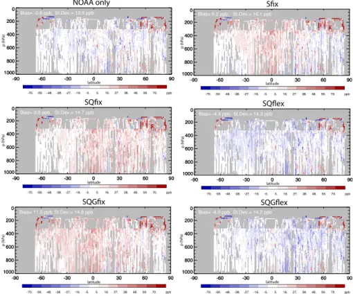
3.1.2 SCIAMACHY vs. NOAA-only

Next we investigate whether the SCIAMACHY bias cor-rections improve the consistency of the NOAA-only opti-mized model. Figure 5 shows maps of the residual ences between the two, averaged seasonally. These differ-ences can be interpreted as the signal that is brought in by SCIAMACHY, in addition to what is provided by the sur-face network. At temperate latitudes the residuals are on av-erage −30 ppb, roughly consistent with the 2 %

(9)

4

Fig. 4.Comparisons between detrended TCCON and inversion-derived seasonal cycles ofXCH4averaged over TCCON sites in the Northern

Hemisphere (left) and Southern Hemisphere (right). Black: TCCON, red: NOAA only, green:S_fix corrected SCIAMACHY, blue: SQ_fix

corrected SCIAMACHY.

SQGfixbias correction leads to a systematic overestimation

ofXCH4compared to the NOAA-only inversion (13 ppb on

average), which is largely reduced if the scaling factors are further optimized in the SQGflexinversion (−5 ppb on

aver-age). This result can be explained by the general tendency of the NOAA-only inversion to slightly underestimate TCCON. Note that the differences that remain after bias correction in Fig. 5 include real signals of methane sources that are not represented by the NOAA-only inversion.

3.1.3 Extended comparison to TCCON

The SCIAMACHY calibration using TCCON mainly repre-sents the period after the launch of GOSAT (2009–2010), when most sites became operational. It raises the question of whether the inferred bias corrections are valid also for other years. With only a limited number of available TCCON sta-tions for years prior to 2009, this is difficult to assess. Nev-ertheless, an attempt is made as shown in Fig. 6. Reasonable agreements are found, except that the “flex” inversions show systematic underestimation of the TCCON measurements, which is seen most prominently at Darwin. The NOAA-only inversion underestimates TCCON also, with system-atic differences increasing towards southern latitudes (3 ppb for Park Falls, 10 ppb for Lauder). This finding is in line with Monteil et al. (2013), who point to inaccuracies in the TM5 simulated atmospheric transport or the chemical oxi-dation of methane, which are not optimized in the current inversion setup. It should be realized that the aircraft mea-surements for calibrating the TCCON network cover only a small fraction of the presented time series, and therefore the calibration of the TCCON-observed inter-annual variability has its limitations also. The comparison at Park Falls shows clear examples of the phase-shifted seasonality of theSfix

corrected SCIAMACHY data, in particular during the first months of 2005 and 2006. Overall, the SQfixinversion shows

the best agreement with the three long-term TCCON time series (rms=9.0 ppb), followed by SQG_fix(rms=9.6 ppb).

3.1.4 Statistics of fit residuals

Next, we analyse the distributions of residuals between the optimized models and the NOAA measurements that were used in the inversions (see Fig. 7). Deviations from a Gaus-sian distribution centred around the origin may point to re-maining inconsistencies between the bias-corrected SCIA-MACHY data and the surface measurements. As can be seen, the a priori model systematically overestimates the measurements. The NOAA-only inversion shows on aver-age the smallest residuals. This result is expected, since this inversion fits the surface measurements, without constraints to also fit satellite retrievals. SCIAMACHY inversions with fixed biases lead to systematic overestimation of the NOAA flask measurements, which is effectively corrected in the “flex” inversions by reducing the uniform bias component (see Table 3). Of the alternative SCIAMACHY bias correc-tions that were tested, SQGflexand SQflexshow the smallest

residuals, with little difference in performance between these two.

3.2 Performance evaluation using independent data

Aircraft measurements are particularly useful for evaluating inversion optimized concentration fields, since they address the modelled vertical profile of CH4, which connects the

(10)

Fig. 5.The difference inXCH₄between SCIAMACHY and NOAA-optimized TM5 (SCIAMACHY – TM5) with and without SCIAMACHY

bias correction. Results represent seasonal averages for DJF (left) and JJA (right). Top: uncorrected SCIAMACHY, middle: SQGfixcorrected

SCIAMACHY, bottom: SQGflexcorrected SCIAMACHY. For the corresponding bias coefficients see Table 2.

between the planetary boundary layer and the tropopause. The HIPPO measurements were taken from campaigns 1– 3, which took place between January 2009 and April 2010. The comparisons between model and measurements for these campaigns are combined in one figure. The HIPPO measure-ments have been linked to the NOAA scale using coincident measurements from discrete samples collected during the flights and analysed at NOAA. The remote Southern Hemi-sphere offers a good opportunity to verify this approach, since the concentration gradients in the marine boundary layer are small. Therefore a good agreement is expected be-tween the NOAA optimized model and the HIPPO measure-ments. Indeed, at latitudes southward of about 30◦_S

differ-ences are within 3 ppb.

The differences between Sfix and HIPPO show the

ex-pected pattern of over- and underestimation of respectively tropical and extra-tropical CH4 in absence of a latitudinal

varying SCIAMACHY bias correction. When such correc-tions are applied the latitudinal differences reduce, although minor differences remain (within∼10 ppb). The inversions

with the fixed, TCCON-derived, bias corrections tend to overestimate the HIPPO measurements by 6–12 ppb. Fur-ther optimization of the bias coefficients in the inversion

im-proves the agreement with HIPPO, with a low bias of close to 5 ppb. When comparing the results in Figs. 6 and 8 it be-comes clear that surface and aircraft data support lower CH4

mixing ratios than TCCON. This happens despite the fact that TCCON has been validated using aircraft measurements also (see e.g. Deutscher et al., 2010; Wunch et al., 2010; Geibel et al., 2012). The remaining differences could be ex-plained by the stratospheric contribution to the total column, which is the subject of ongoing investigations (see Mon-teil et al., 2013). The residuals between HIPPO and TM5 point to overestimated mixing ratios in the lower stratosphere at higher latitudes (> 50◦_{). The SCIAMACHY retrievals at}

(11)

4

Fig. 6. Comparison between inversion-derived and

TCCON-observedXCH4, at sites with multiple years of data. Black:

TC-CON; red: NOAA inversion; green:S_fix inversion; blue: SQG_flex

inversion. Error bars represent the standard deviation of the plotted diurnal averages.

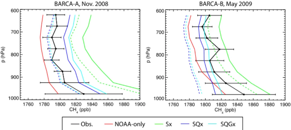
adequate to resolve regional gradients within the Amazon basin. Overall, the results confirm the conclusions from Beck et al. (2012) that using of only surface data in the inversion leads to underestimated posterior mixing ratios. Including SCIAMACHY increases the mixing ratios over South Amer-ica, to an extent which varies considerably between the dif-ferent bias correction approaches. Using only a uniform scal-ing factor leads to overestimated mixscal-ing ratios. The SQ and SQG inversions are in closer agreement with the measure-ments. The relative performance of the “flex” and “fix” inver-sions differs between the two campaigns. Whereas the “flex”

inversions are in close agreement with measurements from the BARCA-A campaign, they tend to underestimate the ob-served mixing ratios during BARCA-B. None of the inver-sions are capable of capturing the seasonal dynamics of the BARCA measurements. The seasonal bias correction hardly influences the difference between BARCA 1 and 2, because the ECMWF-derived regional humidities for the end of the dry and wet season are rather similar.

3.3 Inversion-estimated fluxes

In this section we analyse the inversion-derived surface fluxes of CH4, and their sensitivity to the SCIAMACHY bias

correction. We concentrate on fluxes that are integrated annu-ally and over large enough regions to avoid interpretation of results that are compromised by the generally limited spatio-temporal resolution of the global inversions. Figure 10 shows flux time series for the period of July 2003 to July 2010 for six large regions. Monthly time series of annual fluxes are derived using a boxcar filter with a width of a year. The un-certainties represent 2σ intervals of the annual uncertainty for each region, computed by integrating the posterior covari-ance matrix in space and time, in 6-month intervals. The first and final half years of the inversion time window have been removed to avoid influences of inversion up and spin-down, and end effects of the box car filter. Note that each line is a composite of three 4-year inversions since the full period is split up in three overlapping blocks (as described in Sect. 2). The 2-year overlap allows us to reduce end ef-fects of each of these blocks. Full time series are constructed by connecting the blocks in the middle of the overlapping periods. The NOAA-only and “fix” inversions show insignif-icant jumps between the blocks. For the “flex” inversions, differences are larger because the optimized bias correction parameters in subsequent blocks may differ. Nevertheless, these differences remain small compared with the inversion-derived inter-annual variability.

Compared with the a priori fluxes, the a posteriori fluxes show increased inter-annual variability (IAV), by 40 % for NOAA-only and 70 % for the SCIAMACHY inversions for the regions and data shown in Fig. 10. This increase may in part be real, since the a priori fluxes do not account for some sources of inter-annual variation, such as the year-to-year variation in wetland area. In addition, we do not ac-count for inter-annual variability in the OH sink. As the sink is not optimized in our inversion, the influence of its IAV on the observed mixing ratios is projected on the sur-face fluxes. Studies of OH using methyl chloroform point to inter-annual variations within±_{5 % (see e.g. Holmes et al.,}

2013), which corresponds to variations in methane oxidation of about 25 TgCH4yr−1. This is significant, but also difficult

to account for in global inversions since the available a pri-ori estimates vary substantially and the CH4 measurements

(12)

-60 -40 -20 0 20 40 60 model-obs. (ppb) 0 50 100 150 200

number of measurements (bin

-1)

-60 -40 -20 0 20 40 60

model-obs. (ppb) 0 50 100 150 200 250

number of measurements (bin

-1)

A priori NOAA-only SQGflex Sx SQx SQGx

Fig. 7.Frequency distribution of fit residuals between surface measurements and optimized TM5. (Left panel) Red: a priori; green: NOAA

inversion; blue: SQG_flex. (Right panel) Red:S; green: SQ; blue: SQG. Bold lines: flex scenarios; thin lines, fix scenarios.

-90 -60 -30 0 30 60 90 1000 800 600 400 200 0