Capacidade de regeneração da floresta tropical amazônica sob deficiência nutricional: resultados de um estudo numérico da interação biosfera-atmosfera

(1)

CAPACIDADE DE REGENERAÇÃO DA FLORESTA TROPICAL AMAZÔNICA SOB DEFICIÊNCIA NUTRICIONAL: RESULTADOS DE UM ESTUDO NUMÉRICO DA INTERAÇÃO BIOSFERA-ATMOSFERA

Tese apresentada à Universidade Federal de Viçosa, como parte das exigências do Programa de Pós-Graduação em Meteorologia Agrícola, para obtenção do título de Doctor Scientiae.

VIÇOSA

(2)

Ficha catalográfica preparada pela Seção de Catalogação e Classificação da Biblioteca Central da UFV

T

Senna, Mônica Carneiro Alves, 1981-

S478c Capacidade de regeneração da floresta tropical amazônica 2008 sob deficiência nutricional: resultados de um estudo numéri-co da interação biosfera-atmosfera / Mônica Carneiro Alves Senna. – Viçosa, MG, 2008.

xi, 126f.: il. (algumas col.) ; 29cm.

Orientador: Marcos Heil Costa.

Tese (doutorado) - Universidade Federal de Viçosa. Referências bibliográficas: f. 109-126.

(3)

CAPACIDADE DE REGENERAc;AO DA FLORESTA TROPICAL AMAZONICA SOB DEFICIENCIA NUTRICIONAL: RESULTADOS DE UM E TUDO NUMERICO DA INTERAc;AO BIOSFERA-ATMOSFERA

Tcse apresentada

a

Universidade Federal de Viyosa, como parte das cxigencias do Programa de P6s-Graduay3.o em Meteorologia Agricola, para obtenyao do titulo de Doctor Scientiae.

APROVADA: 22 de abril de 2008.

Prof. Alistides Ribeiro

arcos Daisuk Oyama

/ ~ ~ ~

(4)

O prêmio de uma boa ação é tê-la praticado. Se aproveitares bem o dia de hoje, dependerás menos do de amanhã. (Sêneca)

(5)

AGRADECIMENTOS

A Deus, pelo dom da vida, pela saúde, força, proteção, amor e sabedoria dadas no decorrer de toda a minha vida.

Ao meu marido, Thomaz Schröder Senna, pelo amor e carinho sempre presente em momentos de alegria ou dificuldade. Sem você tudo fica sem sentido. Te aminho muitão!

Aos meus pais, pelo apoio constante e pelos sacrifícios. Obrigada pela confiança depositada em mim.

Ao meu orientador, Professor Marcos Heil Costa, e aos co-orientadores, por todos os ensinamentos, atenção, incentivos e pelas valiosas sugestões dadas no decorrer deste trabalho.

À amiga Gabrielle, por toda ajuda nos scripts de NCL, pela amizade e por toda dedicação e capricho. É bom saber que posso contar com você!

Aos amigos de trabalho Varejão, pela disposição e boa vontade nos ensinamentos de NCL; Clever, pela ajuda constante no Illustrator; Luciana e Lucía, pelos mapas de precipitação e radiação solar; Francisca, pelas sugestões e companheirismo; Hewlley,

(6)

pelos gráficos de calibração do IBIS; Edson e Thomé, pelas conversas, lanchinhos e pelos risos; e a todos os outros do grupo de pesquisa pela boa convivência e descontração.

A todos os demais professores, colegas e funcionários do Departamento de Engenharia Agrícola e Ambiental da UFV, pelo apoio e amizade.

(7)

BIOGRAFIA

MÔNICA CARNEIRO ALVES SENNA, filha de Esperidião Alves Xavier Filho e Jacel Carneiro de Figueiredo Alves, nasceu em 08 de abril de 1981, na cidade de Cruzeiro do Sul – AC.

Em dezembro de 1997 concluiu o curso técnico em Meteorologia pelo Centro Federal de Educação Tecnológica Celso Suckow da Fonseca (CEFET-RJ).

De janeiro de 2000 a novembro de 2001 trabalhou como Técnica em Meteorologia na Fundação Instituto Geotécnica do Município do Rio de Janeiro (GEO-RIO).

Em março de 2002 concluiu o curso de graduação em Meteorologia pela Universidade Federal do Rio de Janeiro (UFRJ).

Em fevereiro de 2004 concluiu o curso de pós-graduação, em nível de Mestrado, em Meteorologia Agrícola na Universidade Federal de Viçosa (UFV).

Em fevereiro de 2004 iniciou o curso de pós-graduação, em nível de Doutorado, em Meteorologia Agrícola na Universidade Federal de Viçosa (UFV), dedicando-se ao estudo das interações atmosfera-biosfera.

(8)

RESUMO

SENNA, Mônica Carneiro Alves, D.Sc., Universidade Federal de Viçosa, abril de 2008.

Capacidade de regeneração da floresta tropical amazônica sob deficiência nutricional: resultados de um estudo numérico da interação biosfera-atmosfera. Orientador: Marcos Heil Costa. Co-Orientadores: Carlos

Afonso Nobre e Luiz Cláudio Costa.

Essa tese investiga como as retroalimentações do clima e da disponibilidade de nutrientes no solo interagem na regulação dos padrões de recrescimento da floresta tropical amazônica após um desmatamento de grande escala. Nesse estudo foi utilizado o modelo acoplado biosfera-atmosfera CCM3-IBIS. Inicialmente, o modelo foi validado através de observações de variáveis climáticas e de dinâmica e estrutura da vegetação amazônica. O clima da Amazônia (média anual e sazonalidade) é muito bem simulado tanto para a precipitação quanto para a radiação solar incidente. Os padrões de cobertura vegetal representam bem os padrões observados. A produção primária líquida e as taxas de respiração simuladas diferem em 5% e 16% das observações, respectivamente. O desempenho das variáveis simuladas que dependem da alocação de carbono, como a partição da produção primária líquida, o índice de área foliar e a biomassa, é alto em uma média regional, mas é baixa quando são considerados os padrões espaciais. Uma

(9)

melhor representação desses padrões espaciais depende da compreensão da variação espacial da alocação de carbono e sua dependência com fatores ambientais. Para avaliar a capacidade de recrescimento da floresta foram realizados dois experimentos. O primeiro experimento considera diferentes tipos de limitação nutricional e um hipotético desmatamento total. O segundo experimento considera o tipo de limitação nutricional mais realístico e diferentes cenários de desmatamento, com o intuito de encontrar um limite máximo de desmatamento que não causaria interferências prejudiciais na regeneração da floresta. Os resultados mostram que a redução da precipitação é proporcional à quantidade de desmatamento e é mais drástica quando mais do que 40% da extensão original da floresta é desmatada. Além disso, apenas a redução da precipitação simulada não é suficiente para impedir a regeneração da floresta secundária. Entretanto, quando a redução da precipitação é associada com uma deficiência nutricional do solo, um processo de savanização pode ocorrer sobre o norte do Mato Grosso, independente da extensão da área desmatada. Esses resultados são preocupantes, pois essa região tem as mais altas taxas de desmatamento da Amazônia. A baixa resiliência da floresta com deficiência nutricional indica que o norte do Mato Grosso deveria ser o alvo principal de iniciativas para a conservação.

(10)

ABSTRACT

SENNA, Mônica Carneiro Alves, D.Sc., Federal University of Viçosa, April 2008.

Amazon rainforest regrowth under nutrient stress: results from a biosphere-atmosphere interaction numerical study. Adviser: Marcos Heil Costa.

Co-Advisers: Carlos Afonso Nobre and Luiz Cláudio Costa.

This thesis investigates how the climate feedback and the nutrient feedback interact to regulate the patterns in the regrowth of the Amazon tropical forest after a large-scale deforestation. The study is performed using the fully coupled biosphere-atmosphere model CCM3-IBIS. Initially, the model was validated against observed climate and vegetation dynamics and structure variables. The Amazon climate (annual mean and seasonality) is extremely well simulated for both precipitation and incident solar radiation. Vegetation cover patterns reproduce well the observed patterns. The simulated net primary production and respiration rates are within 5% and 16% of observed data, respectively. The performance of simulated variables that depend on carbon allocation, like net primary production partitioning, leaf area index and biomass, although good on a regional mean, is low when spatial patterns are considered. A better representation of these spatial patterns depends on the understanding of the spatial variation in carbon allocation and its relationship to environmental factors. To evaluate

(11)

the rainforest regrowth two experiments were done. The first experiment considers different types of nutrient stress and a hypothetical full deforestation. The second experiment considers the most realistic type of nutrient stress and different deforestation scenarios, looking for a threshold of deforestation that could cause dangerous interference on the Amazon recovery. Results show that the reduction in rainfall is proportional to the amount of deforestation and is more drastic when the deforested area is higher than 40% of the original forest extent. In addition, this simulated precipitation reduction alone is not sufficient to prevent the rainforest regrowth. However, when the precipitation reduction is associated with a soil nutrient stress, a savannization process may start over northern Mato Grosso, no matter how much is deforested. This is concerning because this region has the highest clearing rates in Amazonia. The low resilience of the forest under nutrient stress indicates that northern Mato Grosso should be a major target for conservation initiatives.

(12)

GENERAL INTRODUCTION

The Amazon tropical forest is the world’s largest rainforest, an ecosystem that

supports perhaps 30 percent of terrestrial species [Godoy et al., 1999; Prance et al.,

2000; Dirzo and Raven, 2003], and plays a crucial role in the climate system,

particularly as a driver of atmospheric circulation [Zeng and Neelin, 1999; Costa and

Foley, 2000]. Recent studies have suggested that the Amazon may reduce in extension

and lose biomass during the 21st century through a savannization process [Magrin et al.,

2007]. In addition, changes in the carbon balance of this region could have significant

effects on the global carbon cycle and on the greenhouse effect [Denman et al., 2007;

Bala et al., 2007].

Over the last few decades, high rates of deforestation have been occurring in the

region [Skole and Tucker, 1993; Nepstad et al., 1999; INPE, 2007]. The reasons for

land-clearing in the Amazon are compelling: cheap land, low labor costs, booming

demand for commodities driven by a surging China, and growing interest in biofuels. In

less than a generation, these factors have helped Brazil become a large exporter of beef,

(15)

land values double every 4-5 years in areas that just a decade ago were rainforests. The

market is driving deforestation [Soares-Filho et al., 2006; Nepstad et al., 2006].

This conversion of forests to agricultural land is more than just the loss of trees.

The deforestation also affects species composition, productivity, and biomass along

edges and in remaining fragments, and can influence the likelihood of fires [Laurance et

al., 1997; Mesquita et al., 1999; Cochrane et al., 1999; Nepstad et al., 2001].

Early studies focused on climate change induced by deforestation [Nobre et al.,

1991; Hahmann and Dickinson, 1997; Lean and Rowntree, 1997; Costa and Foley,

2000], whereas coupled changes of climate and vegetation [Levis et al., 2000; Cox et

al., 2004] are the current interest. The majority of biosphere-atmosphere studies in

Amazonia investigate the sensitivity of climate to the full Amazon deforestation, which

is not a realistic scenario. Two recent studies, however, evaluate the response of the

Amazonian climate to the partial deforestation [Costa et al., 2007; Sampaio et al.,

2007], concluding that the precipitation reduction in this region is more evident when

deforestation exceeds 40-50% of the original forest cover.

As deforestation of tropical forests continues, one of the future hopes for these

damaged ecosystems is the regeneration of secondary forests. Some areas that were

once slash-and-burned for cattle ranching or subsistence agriculture have been

abandoned, allowing scientists to study the possibility of recovery in the rainforest.

Amazonian regrowth forests are an important reservoir of genetic diversity of forest

species [Vieira et al., 2003] and have a substantial role in sequestering carbon [Zarin et

al., 2001]. This secondary forest regrowth, however, may be limited by climate and

nutrient availability.

(16)

weathered, nutrient impoverished and acidic soils of the Amazon are a challenge to

plant growth. Further soil degradation and nutrient loss through intense land-use and

frequent fires may result in reduced growth rates in successional species [Davidson et

al., 2004; Zarin et al., 2005]. However, after decades of regrowth in a conservative

nutrient cycling legacy, the secondary forest rebuilds nutrient stocks in advanced

successional and mature stages [Davidson et al., 2007] because most of the rainforest

essential nutrients are locked up in the living vegetation, dead wood, and decaying

leaves. As organic material decays, it is quickly recycled.

Although research shows the effects of changing precipitation and changing

nutrient status on the forest regrowth, we still do not know how these factors interact to

regulate the forest regrowth and if these interactions vary in different parts of

Amazonia. Considering these issues, the objective of this thesis is to investigate these

feedbacks in the Amazon region using the fully coupled climate-biosphere model

CCM3-IBIS. This study is organized as follows: Chapter 1 investigates how well this

fully coupled model can reproduce vegetation structure and dynamics in Amazonia, to

the extent permitted by available data. Chapter 2 studies how the climate and nutrient

feedbacks may affect the forest regrowth after a hypothetical full deforestation,

considering two types of nutrient stress (fixed vs. dynamic). Chapter 3 investigates how

the climate and nutrient feedbacks may alter the rainforest regrowth after different

deforestation scenarios from Soares-Filho et al. [2006] and Sampaio et al. [2007],

which assume that recent deforestation trends will continue in the next

(17)

CHAPTER 1 CHALLENGES OF A COUPLED CLIMATE-BIOSPHERE MODEL

TO REPRODUCE VEGETATION STRUCTURE AND DYNAMICS

(18)

1.1. INTRODUCTION

Terrestrial biosphere and climate interact through several complex feedbacks.

The global pattern of natural vegetation cover is governed by climate through

precipitation, solar radiation, temperature and CO2 concentration [Prentice, 2001;

Nemani et al., 2003; Liu et al., 2006]. Changes in climate may alter competitive relationships among species, and thus may alter the structure and biogeography of

ecosystems. On the other hand, changes in community composition and ecosystem

structure may alter the fluxes of energy, water, momentum, CO2, and other atmospheric

gases, consequently affecting climate [Pielke et al., 1998; Bonan, 2002; Foley et al.,

2003].

The interactive coupling of terrestrial ecosystems and climate has been

examined by fully integrated dynamic global vegetation models within global climate

models [Betts et al., 1997; Foley et al., 1998, 2000; Bonan et al., 2003; Krinner et al.,

2005]. In these coupled models, vegetation growth and biogeography are influenced by

temperature, precipitation, and other climate variables. In turn, vegetation height, leaf

area, rooting depth, and other vegetation parameters influence albedo, radiative

(19)

also incorporate processes such as mortality and competition among plant functional

types [Bonan, 2002; Moorcroft, 2003].

Several coupled climate-biosphere models have been applied to problems of the

global carbon cycle [Cox et al., 2000; Friedlingstein et al., 2001, 2006] and climate

change [Betts et al., 1997; Brovkin et al., 1999; Foley et al., 2000; Liu et al., 2006;

Notaro et al., 2007]. The initial climate projections with a coupled ocean-vegetation-atmosphere general circulation model that consider carbon exchanges

among the oceans, land, and atmosphere showed that the overall effect of

carbon-climate interaction is a positive feedback, mostly due to the negative impacts of

climate change on land carbon storage [Cox et al., 2000; Friedlingstein et al., 2001], but

the magnitude of this feedback varied a lot between these studies. Results from the

Coupled Climate-Carbon Cycle Model Intercomparison Project (C4MIP) show a

unanimous agreement among all the 11 models that the climate-carbon cycle feedback

is positive [Friedlingstein et al., 2006]. However, large disagreement remains on the

magnitude of this feedback strength, as well as on the regional aspects of this feedback.

A major uncertainty in the carbon budget relates to changes in the carbon stocks

of tropical forests. Old growth tropical forests contain large stores of live biomass, soil

organic matter, and are very dynamic, accounting for a major fraction of global net

primary production and global live biomass. Changes in the carbon balance of these

regions could have significant effects on global CO2 [Denman et al., 2007; Bala et al.,

2007].

Of the tropical forest regions, the Amazon is of primary importance, not only

because it contains more than half of the world’s tropical rainforests, but also because

(20)

report, have suggested that it may reduce in extension and lose biomass during the 21st

century [Magrin et al., 2007] through a savannization process.

Despite such predictions, the models involved have not been fully validated

against the available field and remote sensing measurements that characterize the

vegetation dynamics of the region. In this study, we investigate how well a fully

coupled atmosphere-biosphere model can reproduce vegetation structure and dynamics

in Amazonia. Evaluating and improving the representation of the vegetation structure,

dynamics and carbon cycle of Amazonia in coupled atmosphere-biosphere models will

increase our ability to understand the impacts of land-use changes on the global carbon

cycle and to perform reliable projections of future climate changes.

The accurate representation of the coupled climate-biosphere dynamics requires

the accurate representation of climate, net primary production, and its partition among

the several carbon pool components. We focus the climate analysis on precipitation (P)

and incident solar radiation (Sin), because they are the most important climate variables

for Amazon vegetation dynamics, and we validate the resulting land cover and other

(21)

1.2. MATERIALS AND METHODS

1.2.1.Model Description

In this study we use the coupled climate-biosphere model CCM3-IBIS, which is

virtually the same core model of the LLNL (Lawrence Livermore National Laboratory)

model used in the C4MIP project, except for our own tuning for the rainforest (described

below). The atmospheric component of the coupled model is the NCAR Community

Climate Model (CCM3) version 3.6.16 [Kiehl et al., 1998]. CCM3 is an atmospheric

general circulation model with spectral representation of the horizontal fields. It

simulates the large-scale physics (radiative transfer, hydrologic cycle, cloud

development, thermodynamics) and dynamics of the atmosphere. In this study, we

operate the model at a spectral resolution of T42 (~2.81º X 2.81º latitude/longitude

grid), 18 vertical levels, and a 15-min time step. The oceans are represented by monthly

averaged fixed sea-surface temperatures of the 1990s that serve as boundary conditions

for the atmosphere.

CCM3 is coupled to the Integrated Biosphere Simulator (IBIS) version 2.6.4

(22)

processes occurring in vegetation and soils. IBIS simulates land surface processes, plant

phenology and vegetation dynamics, and represents vegetation as two layers (trees and

grasses). In IBIS a grid cell can contain one or more plant functional types (PFTs) that

together comprise a vegetation type. Land surface physics and canopy physiology are

calculated at the same time step used by CCM3. The plant phenology algorithm has a

daily time step and the vegetation dynamics is solved with an annual time step. IBIS is a

0-dimensional model that operates on each CCM3 land surface grid point. When

dynamic vegetation component is enabled, vegetation structure and biogeography

change in response to climate. A detailed description of the model follows, as relevant

to the validation.

IBIS represents vegetation dynamics using very simple competition rules. The

relative abundance of 12 PFTs in each grid cell changes in time according to their

ability to photosynthesize and use water. Thus the model can mechanistically simulate

the competition between different plant forms. The competition between plant types of

the same basic form is driven by differences in the annual carbon balance resulting from

differences in phenology, leaf form, and photosynthetic pathway.

IBIS calculates roots maintenance respiration (Rroot) as a function of the carbon

contained in root biomass and the soil temperature in the rooting zone. The efflux of

carbon from the soil, including the litter decomposition (Rsoil+litter), is the sum of Rroot

and carbon that is respired by the microbial biomass (Rheterotrophic) during its oxidation of

the soil organic matter. Rheterotrophic depends on soil moisture and temperature, and on the

amount of available substrate.

Total net primary production (NPPtotal) is calculated integrating primary

production through the year discounting maintenance respiration and the carbon lost due

(23)

and roots (Cr). Changes in the carbon pool i (Ci) are described by the differential equation i i i total i i C C NPP a t C .

. −

τ

−δ

= ∂ ∂

(1)

where ai represents the carbon allocation coefficient of leaves (al), wood (aw), and roots

(ar); τi describes the residence time of carbon in leaves (τl), wood (τw), and roots (τr). In

IBIS, ai and τi are assumed to be fixed in space and time within a given PFT. is a

generic parameter for disturbances, such as fires, herbivory, etc., which is set to zero in

this simulation.

NPPtotal is divided into belowground and aboveground net primary production

(NPPbg and NPPag, respectively). Aboveground wood net primary production (NPPagw)

is the rate at which carbon is fixed into aboveground woody biomass structures, like

trunks, stems and branches. NPPagw is calculated by multiplying NPPtotal by aw

(Equation (1)).

In IBIS, the changes in leaf display and physiological activity are triggered by

climatic events, when there are one or more unfavorable seasons. Drought deciduous

plants (e.g. tropical deciduous trees) are assumed to respond to changes in net canopy

carbon budget. The leaf area index (LAI) of each PFT is obtained by dividing leaves

carbon (Cl) by specific leaf area. In this study, the specific leaf area for both tropical

evergreen and tropical deciduous trees are set to 17 m2 kg-C-1 [Figueira et al., 2002].

IBIS represents transient changes in biomass directly proportional to the carbon

allocation coefficient – al, aw, and ar – and inversely proportional to the residence time

(from loss of biomass through mortality and tissue turnover) – τl, τw, and τr – of each

biomass compartment (Equation (1)). Total biomass is divided into belowground

(24)

1.2.2.Model Calibration

The data used for model calibration were collected at four micrometeorological

sites in areas of primary forest of the Large Scale Biosphere-Atmosphere Experiment in

Amazonia (LBA) (Figure 1.1): Jaru (10.8º S; 61.9º W), Manaus (2.6º S; 60.2º W),

Tapajós km 67 (2.9º S; 55.0º W), and Tapajós km 83 (3.1º S; 54.9º W) [Imbuzeiro,

2005; Yanagi, 2006]. We calibrated an offline version of the model, and the optimized

parameters were then transferred to the coupled model. The model is initially optimized

for net radiation exchange (Rn), then for mass and energy fluxes – latent heat flux (LE),

sensible heat flux (H), net ecosystem exchange (NEE). The calibration process involves

a reasonably large number of simulations selecting, in each one of them, values for

specific model parameters. The optimized model parameters and their optimized value

are leaf reflectance in visible and near infrared bands (ρvis, ρnir), orientation of the upper

canopy leaves (χu), coefficient that relates canopy conductance with net photosynthesis

(m), maximum capacity of the Rubisco enzyme at 15°C (Vmax), heat capacity of the

stems (Cs), and a parameter related to the vertical distribution of the root system (β2). In

each simulation, the results of the model output are compared against observed data,

seeking to minimize the root mean square error (RMSE) while keeping an unbiased

(25)

1.2.3.Simulation Setup and Validation Data

Delire et al. [2002, 2003] investigated the basic global climate and carbon cycle simulated by this coupled model and showed that CCM3-IBIS can be used to explore

geographic and temporal variations in the global carbon cycle. In this study, we focus

on the Amazon climate and carbon cycle.

To investigate how well CCM3-IBIS can reproduce vegetation dynamics in

Amazonia, we conduct a simulation for a period of 50 years: the last 20 years are

averaged to analyze the results, while the first 30 years are left for the model to

approach an equilibrium state, specifically with respect to soil moisture and carbon

pools. The land cover is initialized with modern natural vegetation [Ramankutty and

Foley, 1999] and the dynamic vegetation component is enabled. During the simulation,

CO2 concentration was kept constant at 380 ppmv. The initialization values for the

rainforest C pools are 0.38, 10.83, and 0.19 kg-C m-2 for Cl, Cw, and Cr, respectively.

Carbon allocation coefficients for the rainforest are 0.4, 0.4, and 0.2 for al, aw, and ar,

and carbon residence times are 1.01, 25, and 1 year for τl, τw, and τr, respectively.

To minimize initialization period, we have initialized the rainforest carbon pools

with values very close to the equilibrium state, obtained from previous runs. We have

also verified that live C pools were in equilibrium after 30 years in different points of

Amazonia.

We should note here that, since the climate dynamics and the vegetation

structure and dynamics are fully interdependent, a correct representation of both is

required. Otherwise, an error in the simulated climate may introduce and error in the

(26)

The climate produced by CCM3 is validated against precipitation (P) and

incident solar radiation (Sin) data. P and Sin are the two variables most relevant to

vegetation dynamics in the Amazon. We also validate the following vegetation

dynamics variables: heterotrophic respiration (Rheterotrophic), root respiration (Rroot), soil

and litter respiration (Rsoil+litter), net primary production (NPPtotal), aboveground net

primary production (NPPag), and aboveground wood net primary production (NPPagw).

The validated vegetation structure variables are leaf area index (LAI), and aboveground

live biomass (AGLB). The next paragraphs describe each validation dataset.

Simulated precipitation is compared against eight different precipitation

databases, including three climatological surface rain gauge datasets – CRU (Climatic

Research Unit - New et al. [1999]), Legates and Willmott [1990], and Leemans and

Cramer [1990]; three that blend remote sensing data with surface rain gauges – CMAP

(CPC Merged Analysis of Precipitation - Xie and Arkin [1997]), GPCP (Global

Precipitation Climatology Project - Huffman et al. [1997]), and TRMM (Tropical

Rainfall Measuring Mission - Kummerow et al. [1998]); and two reanalysis datasets –

NCEP/NCAR [Kalnay et al., 1996] and ERA-40 [Uppala et al., 2005]. All available

data in the time series are used to describe the precipitation climatology. The use of a

large number of precipitation datasets is important because regional precipitation

estimates in Amazonia are considerably different among themselves [Costa and Foley,

1998].

Simulated incident solar radiation at surface is compared against GOES data as

processed by the algorithm GL1.2 [Ceballos et al., 2004]. This algorithm uses

reflectance in visible channel from GOES 8 for assessing solar flux in two different

broadband intervals (visible and near-infrared), where physical characteristics of

(27)

negligible) term. The GL1.2 algorithm includes cloud cover assessments, water vapor,

carbon dioxide, and ozone absorption. However, it does not include the presence of

aerosols. The series used are from 1997 to 2006.

Land cover is compared against the SAGE (Center for Sustainability and the

Global Environment) potential vegetation dataset, described in Ramankutty and Foley

[1999]. The potential vegetation map is intended to represent the vegetation that would

exist in a location without human intervention.

Rheterotrophic, Rroot, Rsoil+litter, NPPtotal and NPPag are compared against data from

Malhi et al. [submitted], who carefully synthesized results on the carbon stocks, nutrient stocks and particularly the internal carbon allocation in forests in three sites: Manaus

(2.6º S; 60.2º W), Tapajós (2.9º S; 55.0º W), and Caxiuanã (1.8º S; 51.5º W) (Figure

1.1).

NPPagw is compared against a large dataset from Malhi et al. [2004]. These data

were collected at old-growth humid forests with no evidence of major human-induced

disturbance for at least a century. The plots are spread through Brazil, Bolivia, Peru,

Ecuador, Colombia, Venezuela, Guyana, Suriname, and French Guiana, with a good

coverage of Amazonia.

LAI is compared against in situ measurements of ABRACOS (Anglo-Brazilian

Amazonian Climate Observation Study) and LBA forest sites, and remote sensing

estimates from the MODIS MOD-15 product. The data from ABRACOS are annual

mean values of Ji-Paraná (10.1º S; 61.9º W), Manaus (3.0º S; 60.0º W), and Marabá

(5.8º S; 49.2º W) sites (Figure 1.1). Various methods were used to measure and estimate

LAI and there was overall consistency in the estimates for each site [Roberts et al.,

1996]. The data from LBA are monthly mean values of Tapajós site (2.9º S; 55.0º W)

(28)

monthly values of Tapajós site from December 2003 to November 2004. We use the

collection 4 LAI dataset at 1 km spatial resolution.

AGLB is compared against two different datasets. The first one is a spatially

extensive dataset from Malhi et al. [2006], presenting the AGLB of undisturbed

old-growth Amazonian forests plots. The plots are spread through Brazil, Bolivia, Peru,

Ecuador, Colombia, Venezuela, Guyana, Suriname, and French Guiana. The second

one, from Saatchi et al. [2007], combines a large number of AGLB plots and remote

(29)

1.3. RESULTS

1.3.1.Model Calibration

The model parameters that minimized Rn, H, LE and NEE are ρvis = 0.062, ρnir =

0.280, χu = 0.86, m = 8, Vmax = 120 μmol m-2 s-1, Cs = 5.27 x 104 J m-2 K-1, and β2 =

0.997 [Imbuzeiro, 2005, Yanagi, 2006]. Table 1.1 shows the mean relative error (e) and

the root mean square error (RMSE) of simulated H, LE, and NEE before and after

calibration, for the Tapajós km 83 and km 67, Manaus and Jaru sites. The values of e

and RMSE in general decreased when the parameters were calibrated. Figure 1.2 shows

selected charts of the dispersion, cumulative and temporal patterns of H, LE and NEE

for the four sites after calibration. The new set of IBIS parameters produces good results

for hourly variability (Figure 1.2g) and for cumulative pattern along the year (Figure

1.2a, 1.2c and 1.2e) for H, LE and NEE, although the dispersion may vary from site to

(30)

1.3.2.Precipitation

Table 1.2 shows the annual mean P for the Amazon tropical forest region

simulated and calculated from eight different P databases. Annual mean P estimates

vary considerably from 4.98 to 6.70 mm/day. The CCM3-IBIS estimate (6.20 mm/day)

is in the middle of the P dataset range and is within 5% of the ERA-40, Leemans and

Cramer, Legates and Willmott and TRMM datasets. The greater difference is 24.5% for

the CRU dataset.

Figure 1.3 presents the monthly variation of Amazon tropical forest P simulated

by CCM3-IBIS and according to the eight datasets. Simulated P amplitude is within the

amplitude of the datasets, and the seasonality is well simulated too, although it is

advanced in time by one month.

Figure 1.4 illustrates the spatial pattern of annual mean P for South America

simulated and for three selected datasets (Legates and Willmott, Leemans and Cramer,

and TRMM), and the difference between them. CCM3-IBIS (Figure 1.4a) simulates the

main features of South America climate: high P near the equator, with a maximum near

the Brazil-Colombia border, a dry region in Northeast Brazil, the South Atlantic

Convergence Zone (SACZ), the Atacama desert dry climate, a dry region in Pampas,

and a P maximum in southern Chile.

Figures 1.4c, 1.4e, and 1.4g illustrate areas where CCM3-IBIS overestimates

(positive values) or underestimates (negative values) P according to Legates and

Willmott (Figure 1.4b), Leemans and Cramer (Figure 1.4d), and TRMM (Figure 1.4f)

datasets, respectively. In central Amazonia CCM3-IBIS overestimates P according to

Legates and Willmott, and Leemans and Cramer, but not according to TRMM. Due to

(31)

possible that the products Legates and Willmott, and Leemans and Cramer do not

capture spatial patterns of P properly, while the TRMM product should overcome this

limitation. CCM3-IBIS underestimates P over the Guyanas, Amapá and the Marajó

Island in Brazil, and over the Peru-Ecuador border, according to these datasets.

1.3.3.Incident Solar Radiation

The annual mean Sin for the Amazon tropical forest region simulated by

CCM3-IBIS is 227 W/m2, and calculated from GOES GL1.2 is 214 W/m2, with a

difference of 6.1%. Figure 1.5 presents the monthly variation of Amazon tropical forest

Sin simulated and according to the GOES GL1.2 dataset. The simulated amplitude and

seasonality are similar to GOES GL1.2 estimate. The greater differences are in February

and March, but simulated Sin is inside the GOES GL1.2 confidence interval (shaded

area) for all months.

Figure 1.6 illustrates the spatial pattern of annual mean Sin for South America

simulated (Figure 1.6a), for GOES GL1.2 dataset (Figure 1.6b), and the difference

between them (Figure 1.6c). In the major part of the continent, the values are between

200-250 W/m2. CCM3-IBIS represents very well Sin over most of the continent,

although overestimating Sin in western Amazonia, with a maximum over the Andes and

southern Bolivia (Figure 1.6c). There are a few points where the model underestimates

Sin over the Atlantic Ocean, Brazil, Suriname, and Colombia. Over most of Amazon

tropical forest region, though, there is a good agreement between CCM3-IBIS and the

(32)

1.3.4.Land Cover

Figure 1.7 shows the land cover distribution simulated (Figure 1.7a) and from

the SAGE potential vegetation dataset (Figure 1.7b). Despite the low spatial resolution,

CCM3-IBIS successfully reproduces tropical evergreen forest in the Amazon region.

Nonetheless, simulated land cover differs from potential vegetation in some areas. Over

Roraima in Brazil, CCM3-IBIS simulates grassland where the vegetation should be

savanna; over northern Venezuela, eastern Colombia, and southeast Amazonia, the

simulated land cover is tropical deciduous forest while the potential vegetation map

shows the existence of savanna. This is an artifact of the simulation setup because

disturbances are turned off in this simulation. Savanna ecosystems are characterized by

the co-occurrence of trees and grasses, and are strongly influenced by disturbances like

fire. According to Lund-Rizzini hypothesis, a savanna is created by the frequent burning

of a tropical deciduous forest [Lund, 1843; Rizzini, 1979]. This occurs because frequent

fires reduce the woody vegetation cover and favor the grassland expansion. Several

fire-protected savanna experiments in South America [Coutinho, 1982, 1990; San-José

and Fariñas, 1991; Hoffmann, 1996; Henriques and Hay, 2002], Africa [Brookman-Amissah et al., 1980; Trollope, 1982] and Australia [Gill et al., 1981, Lacey et al., 1982] resulted in an increase in tree density and species richness, particularly of fire-sensitive species, evolving towards a tropical deciduous forest community. Theory

suggests that such shifts may be attributed to alternate stable states of savanna/tropical

deciduous forest [Miranda et al., 2002; Scheffer et al., 2005; Lapola, 2007]. A modeling

sensitivity study by Botta and Foley [2002] confirmed these results. They conducted

(33)

rates, finding that frequent disturbances favor grasses over trees, causing large increases

in the geographic extent of savanna in southern and eastern Amazonia.

Despite the general agreement of the major biome distribution, there are a few

regions (a total of three T42 cells) where the simulated land cover is in error. Over

eastern Venezuela and Amapá, the simulated land cover are open shrubland and tropical

deciduous forest, respectively. But the potential vegetation in these areas is tropical

evergreen forest. This misrepresentation is due to precipitation underestimation in these

areas (Figure 1.4). The simulated land cover in the Andes is not realistic because the

sharp elevation gradient of this region introduces heterogeneity in climate and in

vegetation distribution [Botta and Foley, 2002], which is difficult to reproduce in a T42

grid.

1.3.5.Respiration

Table 1.3 presents the Rheterotrophic, Rroot, and Rsoil+litter simulated by CCM3-IBIS

and observed by Malhi et al. [submitted] for the Manaus, Tapajós, and Caxiuanã sites,

and an average over the three sites. The simulated Rheterotrophic is 1.10, 1.02, and 0.81

kg-C m-2 y-1 for Manaus, Tapajós, and Caxiuanã, respectively. CCM3-IBIS

underestimates Rheterotrophic by 14% for Caxiuanã and 32% for Tapajós and overestimates

it by 15% for Manaus. The simulated Rroot for Manaus (0.56 kg-C m-2 y-1) is equal to the

observed value, but the simulated Rroot for Tapajós (0.49 kg-C m-2 y-1) is overestimated

by 32%, and for Caxiuanã (0.38 kg-C m-2 y-1) is underestimated by 49%. The simulated

Rsoil+litter is overestimated by 9% for Manaus and is underestimated by 18% and 29% for

(34)

Although there are large errors in respiration rates at individual sites, an average

over the sites shows an attenuation of these errors. The average simulated respiration

rates are within 15% of the average observed data. A majority of these errors are due to

simplistic representations of Rheterotrophic and Rroot and their dependence on soil

temperature and moisture. Factors such as soil profiles of O2 and CO2, soil pH, the type

of microbial fauna, and the presence of heavy metals, all not parameterized in IBIS,

may affect CO2 production. Moreover, the oversimplification of fine root dynamics can

also contribute to errors in annual estimates of soil CO2 flux [Kucharik et al., 2000].

1.3.6.Net Primary Production and Partition

Table 1.4 shows the NPPtotal, NPPag, and the fraction NPPag/NPPtotal simulated by

CCM3-IBIS and observed by Malhi et al. [submitted] for Manaus, Tapajós, Caxiuanã,

and an average over the three sites. The simulated NPPtotal is overestimated by 22% for

Manaus (1.23 kg-C m-2 y-1) and is underestimated by 19% for Tapajós (1.16 kg-C m-2

y-1) and by 9% for Caxiuanã (0.91 kg-C m-2 y-1). The simulated NPPag is 0.98, 0.92, and

0.73 kg-C m-2 y-1 for Manaus, Tapajós, and Caxiuanã, respectively. The simulated

NPPag is in very good agreement with Caxiuanã observation, but CCM3-IBIS

overestimates NPPag by 34% in Manaus and underestimates it by 19% in Tapajós.

The simulated pattern of NPPtotal and NPPag is similar to the simulated pattern of

respiration rates (Table 1.3), with higher values in Manaus and lower values in

Caxiuanã. The partition of simulated NPPtotal to NPPag is fixed at 80% (aw+al). However,

observed values show a partition of 72% in Manaus and Caxiuanã, and 79% in Tapajós.

CCM3-IBIS underestimates NPPtotal and NPPag in Tapajós, but one should note that the

(35)

conjecture that the Tapajós site has experienced recent major disturbance, and the

reminiscent individuals may be disproportionately allocating carbon to wood production

[Malhi et al., submitted]. This kind of event is not taken into account in this simulation. An average over the three sites shows an excellent agreement between the

simulated and observed NPPtotal and NPPag. Average simulated NPPtotal and NPPag are

within 5% and 2% of the observed data, respectively.

1.3.7.Spatial Patterns of NPP Partition to Wood

Although simulated climate and average NPP patterns are positively evaluated, a

quick analysis of the remaining variables analyzed (NPPagw, LAI and AGLB) shows

important discrepancies. These variables depend on the carbon allocation and residence

time (hereafter CART) coefficients. Realizing the limitation of the a and τ coefficients

used in the initial simulation, we run a sensitivity analysis with additional five

simulations, in which the only changes are in the coefficients a and τ, according to

Table 1.5. In these simulations, climate and NPP are nearly the same, the only changes

are the size of the carbon pools.

In the analyses below (NPPagw, LAI and AGLB), because of the large number of

points involved, we present two kinds of analyses for all six simulations of the

sensitivity study. First, we present basic statistics like the mean error ( ) (Equation (2)),

mean relative error (e) (Equation (3)), and the mean absolute error (MAE) (Equation

(4)). Second, we attempt to investigate whether the spatial distribution of the error is

caused by errors in the simulated climate variables. To do so, we evaluate the

correlation coefficient between the error in NPPagw, LAI or AGLB and the error in Sin or

(36)

∑

− = 1 (Si Oi)

n

ε (2)

∑

− = i i i O O S n

e 1 ( ) (3)

∑

−

= Si Oi

n

MAE 1 (4)

where Si and Oi represent the simulated and observed values, respectively.

Table 1.6 presents the simulated NPPagw averaged over the 21 T42 cells that

have observed data by Malhi et al. [2004] for the six simulations of the sensitivity

study. The simulation a4t25 has the best estimate (0.35 kg-C m-2 y-1) compared to the

mean observed value of 0.30 kg-C m-2 y-1, with the lowest values of , e, and MAE

(0.05 kg-C m-2 y-1, 15.5%, and 0.10 kg-C m-2 y-1, respectively). When wood allocation

coefficient and residence time increase, the mean simulated NPPagw increases and so

does , e, and MAE. For the best simulation (a4t25), the correlation coefficients

between NPPagw error and Sin error (-0.04), and between NPPagw error and P error

according to Leemans and Cramer (0.10), Legates and Willmott (0.20) and TRMM

(-0.09) P datasets, show that the spatial distribution of the NPPagw error is not correlated

to errors in the simulated Sin and P. From these analyses, our interpretation is that the

errors in the spatial variability of NPPagw are not caused by errors in the spatial

simulations of climate, suggesting that the carbon allocation itself may vary spatially.

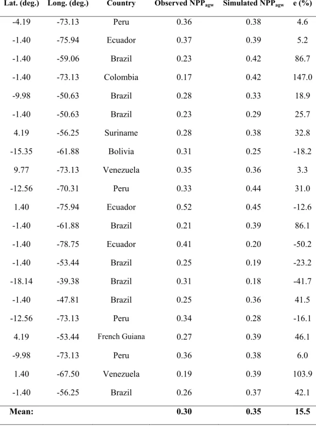
This becomes more clear if we analyze the 21 T42 grid cells individually. Table

1.7 shows NPPagw simulated by CCM3-IBIS for the best simulation (a4t25) and

observed for each cell. The mean simulated NPPagw over these cells is overestimated by

16%, although NPPagw errors calculated at individual sites may be as high as 147% in

Colombia. Malhi et al. [2004] suggest a positive relationship between NPPagw and soil

(37)

shifting balance in carbon allocation between respiration, wood carbon, and fine root

production from site to site. Results from Litton et al. [2007] also indicate that the use

of carbon allocation schemes that vary spatially may provide a more realistic picture of

forest carbon cycling.

CCM3-IBIS assumes that carbon allocation to wood is spatially constant. If the

Malhi et al. [2004] and Litton et al. [2007] conclusions are correct, then the spatial variation in allocation and its relation to environmental variables need to be explicitly

modeled. Representing this process in a model is a challenge, as we still lack the

knowledge of the mechanisms that drive it.

1.3.8.Leaf Area Index

Table 1.8 shows the simulated and observed annual mean LAI for Ji-Paraná,

Manaus, Marabá, and Tapajós. The LAI MODIS estimate is for Tapajós site only. The

a4t25 simulation has the best LAI estimate for all sites, with 7.58, 9.01, 6.91, and 8.93

m2 m-2 for Ji-Paraná, Manaus, Marabá, and Tapajós respectively. This simulation also

has the lowest (2.81 m2 m-2), e (53.1 %), and MAE (2.81 m2 m-2). However, the

overestimation of LAI is very large in all cases, indicating excessive allocation of

carbon to leaves in the model. A cross-analysis of Table 1.4 and 1.8 for the sites of

Manaus and Tapajós indicates that the carbon allocation to leaves indeed vary spatially.

While Tapajós observed NPPtotal is about 43% higher than in Manaus (1.44 vs. 1.01

kg-C m-2 y-1), Tapajós LAI is actually 17% lower than Manaus LAI (5.07 vs. 6.10 m2

m-2). Although this is another evidence that allocation to leaves vary spatially, we

should also consider interannual variations, as these measurements were taken in

(38)

Figure 1.8 illustrates the monthly mean LAI simulated by six CCM3-IBIS

sensitivity simulations, estimated by MODIS, and observed by M. H. Costa

[unpublished data] for Tapajós site. This is apparently the only available ground-based

monthly measurements of LAI in Amazonia. All simulations overestimate the observed

LAI in all months. The a4t25 simulation has the closest estimate. The MODIS estimate

is inside the confidence interval of the observed data only in the dry season (May to

August), a period with the high use of the main algorithm. At other months, MODIS

overestimates LAI because the estimates are contaminated by cloudiness and obtained

via the less reliable secondary algorithm.

1.3.9.Aboveground Live Biomass

Table 1.9 presents the simulated AGLB averaged over the 37 T42 cells of

observed data by Malhi et al. [2006], for the six CCM3-IBIS sensitivity simulations.

The AGLB closest estimate is from a5t40 simulation (16.19 kg-C m-2), with the lowest

(0.99 kg-C m-2) and e (6.5%). The a4t50 simulation has the lowest MAE (2.84 kg-C

m-2), with a close estimate too (14.02 kg-C m-2). When aw and τw increase, the simulated

mean AGLB increases reaching 17.86 kg-C m-2 in a5t50 simulation. For the best

simulation (a5t40), the correlation between AGLB error and Sin error is zero. The

correlation coefficients between AGLB error and P error according to Leemans and

Cramer (0.34), Legates and Willmott (0.29) and TRMM (0.32) P datasets, show a weak

connection between these errors. So, errors in AGLB are not caused by errors in climate

variables.

Table 1.10 shows the simulated AGLB averaged over the 64 T42 cells of

(39)

were excluded from the analysis. Initially, we should note that Saatchi’s et al. average

estimate of biomass (11.2 kg-C m-2) is significantly lower than Malhi’s et al. estimate

(15.2 kg-C m-2). This may be due to errors introduced by the Saatchi et al. algorithm, or

to the sampling by Malhi et al. The simulation a4t25 has the best estimate (9.87 kg-C

m-2) with the lowest , e, and MAE (-1.35 kg-C m-2, -11.7%, and 3.03 kg-C m-2,

respectively). Simulations with higher aw and τw overestimate AGLB. For the best

simulation, the small correlation coefficients between AGLB error and Sin error (-0.04),

and between AGLB error and P error according to Leemans and Cramer (0.17), Legates

and Willmott (0.21) and TRMM (0.26) P datasets, indicate again that the spatial

distribution of the AGLB error is not climate driven, leaving us with the hypothesis that

carbon allocation varies spatially.

Figure 1.9 illustrates the spatial pattern of AGLB for the Amazon region

simulated by six CCM3-IBIS sensitivity simulations, AGLB aggregated from Saatchi et

al. [2007], and the difference between them. Simulated AGLB (Figures 1.9b, 1.9c, 1.9d,

1.9h, 1.9i, and 1.9j) is higher in central Amazonia, Colombia, and in some parts of

Bolivia and Peru. Lower AGLB is simulated over southeast Amazonia. CCM3-IBIS

underestimates AGLB over eastern Venezuela and Amapá in Brazil, because in these

regions the precipitation is underestimated too (Figure 1.4). In eastern Venezuela, the

land cover simulated is not even forest (Figure 1.7), which explains the very low

simulated AGLB.

Figure 1.9e illustrates areas where the best simulation (a4t25) overestimates

(positive values) or underestimates (negative values) AGLB according to Saatchi et al.

[2007] (Figure 1.9a). In southeast Amazonia CCM3-IBIS overestimates AGLB because

this area is deforested and these simulations do not take anthropogenic land use into

(40)

overestimated too. In western Amazonia – parts of Acre, Amazonas, Peru, and

Colombia – CCM3-IBIS underestimates AGLB.

In a5t40 and a5t50 simulations, the simulated AGLB is greater than 17 kg-C m-2

over most of Amazon region (Figures 1.9i and 1.9j). Although the use of these

parameters represent well the high biomass values found by Saatchi et al. at the

Brazil-Peru border, the differences between these simulations and the aggregated map

from Saatchi et al. [2007] (Figures 1.9l and 1.9m) show that in almost all Amazonia

AGLB is overestimated.

Observed AGLB has a significant spatial variability, which may be related to

climate conditions and soil fertility, leading to maximum biomass in wet regions with

low wood productivities and infertile soils (central Amazonia and the Guyana coast),

and lower biomass in dynamic western Amazonia, and the dry southern and northern

Amazon region [Malhi et al., 2006; Saatchi et al., 2007]. For example, wood residence

time is 67 years in central Amazonia, compared to 44 years in western Amazonia

[Malhi et al., 2004]. Since spatial variations in climate are well represented in these simulations, this leaves spatial variations in CART, possibly driven by soil fertility, as

the major reason why spatial patterns of AGLB were not well represented. In order to

have better estimates of the magnitude and the spatial variability of AGLB in the future,

the CART and their relation to environmental variables need to be better understood and

(41)

1.4. DISCUSSION AND CONCLUSIONS

The accurate representation of the coupled climate-biosphere dynamics requires

the accurate representation of climate (in particular P and Sin, the most relevant climate

variables to vegetation dynamics in the Amazon), NPP, and its partition among the

several carbon pools components.

Most variables that do not depend on carbon allocation are simulated within

10% of the estimates: average P is within 5% of four P estimates, average Sin is within

7% of observations, average NPPtotal is within 5% and average NPPag is within 2% of

observations. Respiration rates and NPPagw are within 15% and 16% of the observations,

respectively. Considering only the default run (a4t25), simulated AGLB is within 12%

of Saatchi et al. [2007] estimates, but underestimates Malhi et al. [2006] AGLB by 37%. In both cases, simulated AGLB is underestimated, and LAI is overestimated,

which motivated us to run a sensitivity study, in which higher values of AGLB are

obtained using elevated wood CART parameters.

Although some of these biases could be easily fixed by adjusting a few model

parameters, a larger issue remains, which is the spatial variability of some parameters,

(42)

remove the average LAI bias, but would produce a higher LAI at Tapajós than at

Manaus, while the inverse is observed.

We conclude that the correct simulation of seasonal and spatial patterns of

climate, land cover and NPP does not warrant an accurate representation of the spatial

patterns of vegetation structure and dynamics in Amazonia. Spatial patterns of CART

parameters are needed. To obtain them, there are two possibilities.

The first one is to input the available spatial parameter data [Malhi et al., 2004;

Phillips et al., 2004] into the model. Although this will certainly improve the spatial performance of the model in Amazonia, we still have no clue about the spatial

variability of these parameters in other tropical forest regions of the world. In addition,

the turnover rates (inverse of the residence time) have been increasing in the last 30

years in Amazonia [Phillips et al., 2004], suggesting that this simple parameterization

may not be representative, for example, in a higher CO2 climate.

The second one is to parameterize the known CART coefficients to

environmental variables – the best candidate is soil fertility, according to the data

provided by Phillips et al. [2004] – which creates an additional problem: there are no

global maps of soil fertility, again restricting the application to Amazonia.

On the other hand, the temporal and spatial change of the CART parameters may

be an important adaptative mechanism of the tropical rainforest under climate change.

For example, if the climate becomes drier and there is a trend towards savannization,

plants may respond by allocating more carbon to roots, or forest composition may

change favoring deep root trees instead of tall trees. Moreover, this may happen only in

southern and eastern Amazonia, regions that are in principle more prone to vegetation

(43)

Concluding, this specific coupled climate-biosphere model represents well most

average climate, vegetation structure and dynamics variables in Amazonia – all within

20% of error (with the exception of LAI). Despite this, there are important spatial

differences in the vegetation variables, regardless of good spatial representations of

climate.

Although the current performance is probably sufficient for global experiments

that rely on the region-wide carbon balance, such as C4MIP, the vegetation structure and

dynamics regional performance still needs improvement. This is a challenging research

topic, as there are few studies that measured all components to allow estimation of

partitioning coefficients [Litton et al., 2007]. We also must understand better the

mechanisms that drive them.

Understanding spatial variation in carbon allocation and its relation to climate

and CO2 is a central part of improving the representation of the Amazon spatial patterns.

With a coupled climate-biosphere model that represents well the Amazon structure and

dynamics, we may perform reliable projections of future climate change for this region,

(44)

Table 1.1. The mean percentual relative error (e (%)) and the root mean square error

(RMSE) of simulated sensible heat (H), latent heat (LE), and net ecosystem exchange

(NEE) before and after calibration, for the four sites. The units refer to RMSE only.

From Imbuzeiro [2005].

Calibration Error

H

(W m-2)

LE

(W m-2)

NEE

(kg-C ha-1 hr-1)

e (%) 53 -22 33

Before

RMSE 61.93 118.96 4.41

e (%) 7 6 42

Tapajós km 83

After

RMSE 45.84 98.58 4.02

e (%) 14 7 -99

Before

RMSE 30.60 52.43 5.70

e (%) 11 11 -1

Tapajós km 67

After

RMSE 33.07 52.43 1.13

e (%) 0 4 -216

Before

RMSE 58.70 87.87 6.60

e (%) -4 8 37

Manaus

After

RMSE 45.40 79.34 4.20

e (%) -6 -42 -39

Before

RMSE 81.51 117.20 4.24

e (%) -4 -6 -6

Jaru

After

(45)

Table 1.2. Annual mean precipitation for the Amazon tropical forest region, from

different sources. The mean percentual relative difference (e (%)) is calculated using

each dataset as reference. Dataset values from Pinto [2007].

Precipitation dataset Precipitation (mm/day) e (%)

CRU 4.98 24.5

GPCP 5.36 15.7

CMAP 5.45 13.8

ERA-40 5.91 4.9

Leemans and Cramer [1990] 5.95 4.2

CCM3-IBIS 6.20 -

Legates and Willmott [1990] 6.20 0.0

TRMM 6.39 -3.0

(46)

Table 1.3. Respiration rates (kg-C m-2 y-1) simulated by CCM3-IBIS and observed by Malhi et al. [submitted] for Manaus, Tapajós, Caxiuanã, and an average of the three sites. e (%) is the mean percentual relative error.

Manaus Tapajós Caxiuanã Sites Average

Sim. Obs. e (%) Sim. Obs. e (%) Sim. Obs. e (%) Sim. Obs. e (%)

Rheterotrophic 1.10 0.96 14.6 1.02 1.49 -31.5 0.81 0.94 -13.8 0.98 1.13 -13.6

Rroot 0.56 0.56 0.0 0.49 0.37 32.4 0.38 0.74 -48.6 0.48 0.56 -14.4

Rsoil+litter 1.66 1.52 9.2 1.52 1.86 -18.3 1.19 1.68 -29.2 1.46 1.69 -13.6

(47)

34

Table 1.4. Total and aboveground net primary production (NPPtotal and NPPag, respectively) in kg-C m-2 y-1 and the fraction NPPag/NPPtotal

simulated by CCM3-IBIS and observed by Malhi et al. [submitted] for Manaus, Tapajós, Caxiuanã, and an average of the three sites. e (%) is

the mean percentual relative error.

Manaus Tapajós Caxiuanã Sites Average

Sim. Obs. e (%) Sim. Obs. e (%) Sim. Obs. e (%) Sim. Obs. e (%)

NPPtotal 1.23 1.01 21.8 1.16 1.44 -19.4 0.91 1.00 -9.0 1.10 1.15 -4.3

NPPag 0.98 0.73 34.2 0.92 1.14 -19.3 0.73 0.72 1.4 0.88 0.86 1.5

(48)

Table 1.5. Summary of the CCM3-IBIS simulations used in this study. The simulation

a4t25 was the first, and it is described in materials and methods section. The differences

among the six simulations are the coefficients aw, al, ar, and τw (Equation (1)).

Simulations aw al ar τw (years)

a4t25 0.4 0.4 0.2 25

a4t40 0.4 0.4 0.2 40

a4t50 0.4 0.4 0.2 50

a5t25 0.5 0.4 0.1 25

a5t40 0.5 0.4 0.1 40

(49)

Table 1.6. Simulated and observed mean NPPagw (kg-C m-2 y-1) over the cells from Malhi et al. [2004]. The mean error ( ), mean percentual

relative error (e (%)), mean absolute error (MAE), and the correlation coefficient between NPPagw error and GOES GL 1.2 Sin error (ρ( NPPagw,

Sin)); NPPagw error and Leemans and Cramer P error (ρ( NPPagw, PLC)); NPPagw error and Legates and Willmott P error (ρ( NPPagw, PLW)); and

NPPagw error and TRMM P error (ρ( NPPagw, PTRMM)), are shown for each simulation.

Simulations NPPagw ε e (%) MAE ρ(εNPPagw, εSin) ρ(εNPPagw, εPLC) ρ(εNPPagw, εPLW) ρ(εNPPagw, εPTRMM)

a4t25 0.35 0.05 15.5 0.10 -0.04 0.10 0.20 -0.09

a4t40 0.36 0.06 19.4 0.10 -0.07 0.11 0.23 -0.07

a4t50 0.36 0.06 20.0 0.10 -0.05 0.10 0.23 -0.07

a5t25 0.44 0.14 46.7 0.16 -0.14 0.07 0.20 -0.05

a5t40 0.44 0.14 47.0 0.16 -0.11 0.07 0.20 -0.08

a5t50 0.44 0.14 47.6 0.16 -0.10 0.05 0.19 -0.08

Observation 0.30

(50)

Table 1.7. Observed and simulated NPPagw, and the mean percentual relative error (e

(%)). The simulation used was a4t25, which has the best NPPagw estimate.

Lat. (deg.) Long. (deg.) Country Observed NPPagw Simulated NPPagw e (%)

-4.19 -73.13 Peru 0.36 0.38 4.6

-1.40 -75.94 Ecuador 0.37 0.39 5.2

-1.40 -59.06 Brazil 0.23 0.42 86.7

-1.40 -73.13 Colombia 0.17 0.42 147.0

-9.98 -50.63 Brazil 0.28 0.33 18.9

-1.40 -50.63 Brazil 0.23 0.29 25.7

4.19 -56.25 Suriname 0.28 0.38 32.8

-15.35 -61.88 Bolivia 0.31 0.25 -18.2

9.77 -73.13 Venezuela 0.35 0.36 3.3

-12.56 -70.31 Peru 0.33 0.44 31.0

1.40 -75.94 Ecuador 0.52 0.45 -12.6

-1.40 -61.88 Brazil 0.21 0.39 86.1

-1.40 -78.75 Ecuador 0.41 0.20 -50.2

-1.40 -53.44 Brazil 0.25 0.19 -23.2

-18.14 -39.38 Brazil 0.31 0.18 -41.7

-1.40 -47.81 Brazil 0.25 0.36 41.5

-12.56 -73.13 Peru 0.34 0.28 -16.1

4.19 -53.44 French Guiana 0.27 0.39 46.1

-9.98 -73.13 Peru 0.36 0.38 6.0

1.40 -67.50 Venezuela 0.19 0.39 103.9

-1.40 -56.25 Brazil 0.26 0.37 42.1

(51)

Table 1.8. Annual mean leaf area index (m2 m-2) simulated and observed for Ji-Paraná,

Manaus, Marabá, and Tapajós. The LAI MODIS estimate is for Tapajós only. The mean

error ( ), mean percentual relative error (e (%)), and mean absolute error (MAE) for

each simulation.

Simulations Ji-Paraná Manaus Marabá Tapajós ε e (%) MAE

a4t25 7.58 9.01 6.91 8.93 2.81 53.1 2.81

a4t40 7.72 9.08 7.06 9.08 2.94 55.5 2.94

a4t50 7.88 9.11 7.19 9.13 3.03 57.3 3.03

a5t25 8.51 9.80 7.73 9.75 3.65 69.0 3.65

a5t40 8.43 9.95 7.87 9.94 3.75 70.9 3.75

a5t50 8.56 9.91 7.71 10.06 3.77 71.1 3.77

Observation 4.63 6.10 5.38 5.07

(52)

Table 1.9. Simulated and observed mean AGLB (kg-C m-2) over the cells from Malhi et al. [2006]. The mean error ( ), mean percentual

relative error (e (%)), mean absolute error (MAE), and the correlation coefficient between AGLB error and GOES GL 1.2 Sin error (ρ( AGLB,

Sin)); AGLB error and Leemans and Cramer P error (ρ( AGLB, PLC)); AGLB error and Legates and Willmott P error (ρ( AGLB, PLW)); and

AGLB error and TRMM P error (ρ( AGLB, PTRMM)), are shown for each simulation.

Simulations AGLB ε e (%) MAE ρ(εAGLB, εSin) ρ(εAGLB, εPLC) ρ(εAGLB, εPLW) ρ(εAGLB, εPTRMM)

a4t25 9.55 -5.65 -37.2 5.67 0.20 0.51 0.51 0.44

a4t40 12.54 -2.66 -17.5 3.26 0.07 0.42 0.40 0.40

a4t50 14.02 -1.19 -7.8 2.84 0.03 0.39 0.34 0.37

a5t25 12.38 -2.82 -18.5 3.35 0.11 0.44 0.42 0.40

a5t40 16.19 0.99 6.5 3.56 0.00 0.34 0.29 0.32

a5t50 17.86 2.66 17.5 4.92 -0.03 0.31 0.27 0.31

Observation 15.20

(53)

40

Table 1.10. Simulated and observed mean AGLB (kg-C m-2) over the rainforest cells aggregated from Saatchi et al. [2007]. The mean error

( ), mean percentual relative error (e (%)), mean absolute error (MAE), and the correlation coefficient between AGLB error and GOES GL

1.2 Sin error (ρ( AGLB, Sin)); AGLB error and Leemans and Cramer P error (ρ( AGLB, PLC)); AGLB error and Legates and Willmott P error

(ρ( AGLB, PLW)); and AGLB error and TRMM P error (ρ( AGLB, PTRMM)), are shown for each simulation.

Simulations AGLB ε e (%) MAE ρ(εAGLB, εSin) ρ(εAGLB, εPLC) ρ(εAGLB, εPLW) ρ(εAGLB, εPTRMM)

a4t25 9.87 -1.35 -11.7 3.03 -0.04 0.17 0.21 0.26

a4t40 13.20 2.08 18.1 3.50 -0.10 0.20 0.24 0.32

a4t50 14.82 3.75 32.6 4.33 -0.10 0.20 0.24 0.32

a5t25 12.97 1.85 16.1 3.31 -0.08 0.20 0.25 0.31

a5t40 17.17 6.18 53.6 6.33 -0.13 0.21 0.26 0.34

a5t50 19.06 8.13 70.5 8.19 -0.15 0.22 0.27 0.35

(54)

N

Amazonas

Acre

BOLIVIA PERU

ECUADOR

COLOMBIA

VENEZUELA

GUYANA

SURINAME

FRENCH GUIANA

80°W 70°W 60°W 50°W

10°S 0° 10°N

500 km

Manaus

Ji-Paraná Jaru

Tapajós

Caxiuanã

Marabá Amapá

Roraima

Marajó Island

(55)

Figure 1.2. Dispersion, cumulative and temporal patterns of sensible heat (H), latent

heat (LE), and net ecosystem exchange (NEE) for (a) and (b) Tapajós km 83, (c) and (d)

Tapajós km 67, (e) and (f) Manaus and (g) and (h) Jaru sites, after calibration

(56)

0 1 2 3 4 5 6 7 8 9 10

Jan Feb Mar Apr May Jun Jul Aug Sep Oct Nov Dec

Months

P

rec

ip

it

at

ion

(m

m

/d

a

y)

CCM3-IBIS NCEP/NCAR

ERA-40 CMAP

GPCP TRMM

CRU Leemans and Cramer

Legates and Willmott

Figure 1.3. Monthly variation of precipitation for the Amazon tropical forest region

(57)

Legates and Willmott Difference

Leemans and Cramer Difference

TRMM Difference

CCM3-IBIS

(a)

(b) (c)

(d) (e)

(f) (g)

Figure 1.4. Annual mean precipitation climatology for South America (mm/day) (a)

simulated by CCM3-IBIS, and for (b) Legates and Willmott, (d) Leemans and Cramer,

and (f) TRMM datasets. (c), (e) and (g) The difference is calculated by CCM3-IBIS

minus Legates and Willmott, Leemans and Cramer and TRMM datasets, respectively.

Capacidade de regeneração da floresta tropical amazônica sob deficiência nutricional: resultados de um estudo numérico da interação biosfera-atmosfera

a

/ ~ ~ ~

AGRADECIMENTOS

BIOGRAFIA

RESUMO

ABSTRACT

CONTENTS

GENERAL INTRODUCTION

CHAPTER 1

CHALLENGES OF A COUPLED CLIMATE-BIOSPHERE MODEL

TO REPRODUCE VEGETATION STRUCTURE AND DYNAMICS

1.1. INTRODUCTION

1.2. MATERIALS AND METHODS

τ

1.3. RESULTS

∑

∑

∑

1.4. DISCUSSION AND CONCLUSIONS