NUMERICAL MODEL TO PREDICT
DISTRIBUTION AND EVOLUTION OF
SUSPENDED SEDIMENT TRANSPORT
IN A DAM RESERVOIR
Nacima Hadjrabia Melboucy (1) & Malek Bouhadef (2)
LEGHYD Laboratory – Bab-Ezzouar University – Algiers – Algeria (1) hadjrabia_n@yahoo.fr (2) mbouhadef@usthb.dz
Abstract:
Sediment transport in waterways towards dam reservoirs affects their life span by reducing their storage capacity and burying their bottom control gates and equipments. In this paper, a sediment distribution computed model is presented. It is developed by solving the bi-dimensional horizontal free surface flow ‘Saint Venant equations’ and the depth-averaged mass conservation equation of suspended sediment transport. For that, two explicit finite difference schemes are applied; Mac Cormack for solving hydrodynamic system and upwind for the transport equation. Discretization of 2D equations is done with a rectangular fully dense grid.
The developed model is applied to predict water surface elevation, horizontal components of depth-averaged velocity and sediment transport distribution in Gargar dam reservoir. Computed values are compared with those resulting from Mike21 program and show good agreement with it.
Keywords: Dam silting; finite differences; free surface flow; Sediment transport; Suspended particles.
1. Introduction
In North Africa, specific erosion varies between 2000 and 4000 t/km² [7]. In Algeria, waterways carry sediment concentration about 50 to 150g/l within floods and can get maximum values of 500 to 600g/l. Reservoirs receive annually about 32 million m3 of sediments which leads to annually storage capacity loss about 0.6% [26],[14]. According to literature review, two main ways were used to predict sediment deposits in dam reservoirs. Eroded sediment rate [37] and Trap efficiency [1], [25] and [12]. These methods treat only sediment settlement in reservoirs. A dam design with its constitutive equipments such as bottom outlets has to be optimized considering sediment settlement distribution, in order to minimize their effect on its lifespan.
The purpose of the proposed model is: i) to predict water level evolution, flow velocities and suspended sediment transport in the reservoir, during floods. The calculation of the sedimentation presented here may be a tool for dam design. ii) Comparison and verification of proposed model with Mike 21 code, which is a modeling system of 2D free surface flow and sediment transport, developed by Danish Hydraulic Institute.
Sediment distribution in rivers and lakes and time evolution were considered in predicting models developed since the 1950s, especially for cohesive sediment transport [32].
Cohesive transport simulation models for estuaries and coasts, based on finite differences method such as a one-dimensional model based on transport (Krone, 1962) and erosion (Partheniades, 1965) models [22], a two‐dimensional mixed sediments model [4], a three-dimensional model [31]. Cohesive transport simulation models for water pollution and turbidity were also investigated [27], [20].
Settlement and erosion sediment and bed evolution models in alluvial channels, such as a one dimensional equation system for water and sediment movement in a fully coupled finite differences scheme [23], a 1-D total load mathematical model for long term sediment deposition and erosion in fluvial rivers [18] and bi and tri-dimensional sediment transport and morphological changes in channels simulation model [21].
Bidimensional bed evolution with complex geometry and reservoir sedimentation prediction models based on finite volume method such as: [32], [28], [24].
2. Materials and methods 2.1. Mathematical model
2.1.1. Description of proposed model
A bi-dimensional computation hydrodynamic and transport coupled model was developed for determination of flow hydrodynamic characteristics in the reservoir such as water depth, horizontal components of vertical averaged velocity and suspended sediment concentrations. This mathematical model is based on hydrodynamic Saint Venant and sediment mass conservation equations. Two explicit finite difference schemes, Mac Cormack time-splitting and upwind, are applied for hydrodynamic equations and for transport equation respectively. A fully dense grid is used where all parameters are defined at the same point.
2.1.2. Hydrodynamic model
A depth averaged model based on Saint Venant bi-dimensional equations in conservative form which is the most used in river engineering analysis [11], [36], [28] and [3] is used.The fluid flow equations in reservoirs are the same as those in rivers [32].
Mass conservation equation: 0 (1)
Motion equations:
(2)
(3)
In this hyperbolic equations system, x and y are the horizontal Cartesian coordinates, t time, H flow depth, u
and v depth-averaged flow velocities in x- and y-directions, g gravitational acceleration, S0x and S0ybed slope
components, Sfxand Sfyfriction slope components obtained from Manning’s equation [28]. Bed and friction slope
components are illustrated as follows:
; (4)
(5) Where, n is the Manning coefficient and Zfbed elevation.
Eddy viscosity components εx, εy are defined [6], [15]inzero-equation model:
ε = ⁄ 6 ∗ H (6) Where, = 0.4 is Von Karman’s coefficient, u* is shear velocity defined as ∗ ⁄ , in which, is fluid density and bed shear stress.
2.1.3. Sedimenttransport model
The transported suspended-load withfloodin the reservoir is governed by the two-dimensional depth-averaged mass conservation equation (Convection-diffusion) [13], [32] and [28].
(7)
Where, c is depth-averaged suspended-load concentration, Dx and Dy depth averaged dispersion and diffusion
coefficients in x and y directions respectively, given empirically by (Elder, 1959) and stated in [19], [13] and [8]
Dx = 0.2Hv*+6Hu*, Dy = 0.2Hu*+6Hv* (8)
Where, u* = √(x/) and v* = √(y/) are friction velocity components and by the same way x = gHSfx and y =
gHSfy bed shear stress components.
S is a deposit and/or erosion parameter related to flow shear stress on the bed. In the present work, this parameter is substituted by Sd given by (Krone, 1962) equation in [36].
(9)
Where, Sd is deposit parameter, c sediment concentration, ws is settling velocity,
is deposit stress,
cd criticaldeposit stress, and p deposit probabilities calculated as:
= 0 if > , = 1 if ≤ (10)
Equation (9) was used by many authors [22] and [34].
For low slopes, quadratic terms and of ‘‘Eq. (7)’’ are neglected to become:
(11)
(H u) (H u u) ( ) [ x ( )] [ y ( )] ( o x fx)
t x
H
H uv H u H u g H gH S S
x x y y x
y
(H v) (H u v) ( ) [ x ( )] [ y ( )] (Soy Sfy)
t x
H
H vv H v H v gH g H
y x x y y y
ox Zf x
S SoyZf y
2 2 2 10 3
fx
S
n U U
V
H
2 2 2 10 3fy
S n V U V H
( ) ( ) ( ) [ x ] [ y ]
c c
Hc uHc vHc H D HD S
t x y x x y y
1 . 1
s
d cd cd
S cw
p
1
cd
p
cdp
1
cd
cd² ²
²
²
d
x y
c
c
c
c
c
S
u
v
D
D
t
x
y
x
y
H
This model describes suspended sediment transport in horizontal free surface flow. Sediments are assumed homogenously mixed along the depth; secondary currents, particles cohesion and bed evolution are not considered.
2.2. Numerical model
2.2.1. Hydrodynamic model:
A numerical model based on Mac Cormack finite difference explicit scheme was developed, to solve the Saint Venant hyperbolic and no linear system.
Mac Cormack method is a finite difference time–splitting scheme, with fractional–steps, where the bi-dimensional finite difference operator is simplified to two one-bi-dimensional operators called predictor and corrector. Forward differences are used in the predictor step and backward differences in the corrector step [10]. This scheme is well adapted to free surface flows and well known for its ability to deal simultaneously with computations related to gradually and rapidly varied flows. Many tests showed its performance and accuracy, even in irregular geometry channels and varied bathymetry [11], [10].
2.2.1.1. Application to the bi-dimensional hydrodynamic model
To integrate numerically the partial derivative equations, the continuous physical domain is discretized into a fully dense grid, where dependent variables are defined at the center node, representing mean properties of the grid. In Mac Cormack scheme, the solution in the point (i,j) at t=(n+1)∆t is:
Hn+1ij= Lx(∆tx) Ly(∆ty) Ly(∆ty) Lx(∆tx) Hnij (12) ∆tx = ∆ty= ∆t/2
Where, Lx and Ly are one-dimensional finite difference operators. Each one is applied in two sequences, predictor and corrector, to the hydrodynamic model represented by ‘‘Eq. (1),(2),(3)’’.
2.2.1.2. Mac Cormack scheme Stability
The explicit Mac Cormack scheme is more accurate, when computation time increment Δt is selected respecting the strict equality in the `CFL` (Courant–Friedrichs–Lewy) stability condition, with maximum time step,
∆ 2∆ ⁄ , 2∆ ⁄ (13) In which, ∆x and ∆y are distance increments in horizontal plan, in x and y directions respectively.
2.2.2. Transport model
The finite difference schemes are represented by three approaches: backward, central and forward.
The central derivatives are more precise, not steady and introduce a “wiggle” phenomenon, which may cause divergence in computation [36]. The stability computations have shown that non centralized derivatives on the Upwind side destroy the wiggles, thus:
if ui, j > 0 if ui,j< 0 (14)
2.2.2.1. Upwind application to the transport model
Upwind explicit finite difference scheme is used to solve the suspended mass conservation ‘‘Eq. (11)’’. The discretized equation [19] is then:
(15)
Where, , the mean suspended concentration, Hi,j, ui,j, vi,j are the hydrodynamic field, obtained from the last
sequence of the Mac Cormack scheme, ia, ib, jc, jd are indices, depending on velocity components u and v at considered node:
<0 ia = i+1, ib = i ; >0 ia = i, ib = i-1 (16) <0 jc = j+1, jd = j ; >0 jc = j, jd = j-1
With, and
Upwind scheme stability is verified by CFL condition ‘’Eq (13)’’. The computation domain is defined by the same rectangular mesh (∆x, ∆y) and the same time step (∆t) used for the hydrodynamic model.
2.3. Boundary conditions
There are three kinds of boundary conditions. The first one represents solid boundaries (wall, bank and embankment limiting flow field) where velocity is nil. Fictive symmetrical grids beyond boundaries are introduced, where velocity components (u,v) verify u(i,j-1)=-u(i,j+1) and v(i,j-1)=-v(i,j+1) respectively. For sediment transport, there is no horizontal flux normal to solid boundaries. The second condition represents ‘inlet
, , 1,
i j ci j ci j
c x x
, 1, ,
i j ci j ci j
c x x 1 , , , , , , , , , , - - -- -
-n n n n n n n
i j i j ia j ib j i jc i jd n n i j
i j x y
i j x y
i j
c c c c c c S
u v D c D c
t x y H
u u
v v
1,
- 2
, -1,²
n n n
i j i j i j
n x
c
c
c
c
x
, 1 ,2 , -1- 2
n n n
i j i j i j
n y
c c c
c
y
boundaries’ which are inflow velocity components (u,v) and sediment concentration held from inflow hydrograph and turbidigraph. The third condition represents outlet boundaries, which are spilled height over the spillway, held from outflow hydrograph and sediment concentration supposed equal to zero.
2.4. Computation program
To solve the equations system (1, 2, 3 and 11), the two finite differences schemes mentioned previously were used. The resolution is completed with the initial and boundary conditions. A Fortran Program was developed to simulate the flow and sediment transport in the reservoir.
2.5
.
Model application2.5.1. Description of the study area
Fig.1: Gargar dam situation
Gargar reservoir is situated on Oued Rhiou, located in western of Algeria (Fig.1) which is considered as a semi arid area. It was built in 1988 and its annual inflow is about 185 hm3. Its watershed surface is about 2362 km²; characterized by its form index of 1.8, mean slope of 15.5 m/km and drainage density of 3.9 km/km². Watershed lands are almost bared and only 30% are covered with forests. Gargar reservoir has a great economic importance in the region; it assures water supply for domestic and irrigation needs. Gargar reservoir is also well known for its high sedimentation [2], [16] and [35].
Fig.2: 2-D topography of Gargar Reservoir
Gargar is a 90 m height earth dam, with a crest of 400m length. Its reservoir has a large free water surface of 2100 Ha with an initial capacity of 450 hm3 at normal level of 118 MSL.
A general view of the reservoir form and topography are illustrated in Figure 2. The reservoir overflows through a 60m wide Creager type free surface spillway with a 0.47 flow coefficient.
2.5.2. Modeling procedure
To apply the proposed model, the reservoir area is discretized into a two dimensions finite difference grid system (Fig. 2) with Δx=Δy=50m to 8278 meshes. The time step (Δt) given by the CFL criterion, is lightly variable for different calculation steps and is about 05 seconds. Initial conditions at t=0, are zero for water and
0 20 40 60 80 100 120 140 160 180 200 220 i 0
20 40 60 80 100 120 140 160 180
j
Upstream
Earth Dam Spillway
0 1000
82 86 90 94 98 102 106 110 114 116 118
m
sediment rates on the whole water surface at normal level of the reservoir. Sediment particles are assumed to be an homogeneous fine sand, spherical in shape with 0.04mm diameter and the water/sediment mixture is one phase flow, with a mean density ρ=1.300 kg/m3.
For comparison purposes, Mike21 model is applied to the same case. Eddy viscosity and diffusivity coefficients are considered as the same and calculated by equations (6) and (8) respectively, and settling velocity is supposed zero (ws=0), and bed Manning coefficient n = 0.025.
2.5.3. . Experimental data
A flood occurred in 1994 which hydrographs are illustrated on Figure 3 is considered. Maximum inflow is 1408 m3/s at t=10h; Maximum outflow and spilled height are respectively 153.27 m3/s and Hd=1.47m at t=19h. Flood turbidigraph is plotted on Figure 4; Maximum sediment concentration is 29.08 g/l at t=12h.
Fig 3: Flood hydrographs Fig.4: Flood turbidigraph
3. Results and discussions 3.1.Hydrodynamic model
At t=0h flow rate Q=0 m3/s, velocity components u and v are nil and water level of 118m. Inflow and outflow hydrographs are imposed at reservoir upstream and downstream respectively as inflow and outflow boundaries.
3.1.1. Calculated water depths (m)
Model Mike 21
Fig.5.1: Water depth at 5h Fig. 6.1: Water depth at 5h
0 200 400 600 800 1000 1200 1400
0 10 20 30 40 50 60 70 80 90 100
Discharges m
3
/s
Time (hours) Inflow
Outflow
0 5 10 15 20 25 30
0 5 10 15 20 25 30 35
Time (hours)
concentration
(g/l)
2 0 4 0 6 0 8 0 10 0 12 0 14 16 0 18 0 20 0 22 0
2 4 6 8 10 12 14 16 18
Fig. 5.2: Water depth at 10h Fig. 6.2: Water depth at 10h
Water depth variations for the elaborated model and Mike21 are illustrated in figure 5.1 to 5.3 and 6.1 to 6.3 respectively. At t=5h the water level rises to 118.65m (Fig. 5.1 and 6.1), at t=10h the flow is maximum and water level reached 121.24m (Fig. 5.2 and 6.2); water level decreased to get 120m at t=19h (Fig. 5.3 and 6.3); water level stabilized to normal level of 118m after 4 days.
Fig.5.3: Water depth at 19 h Fig.6.3: Water depth at 19 h
3.1.2. Calculated mean (vectors) velocity (m/s)
Model Mike 21
2 0 4 0 60 80 10 120 140 16 180 20 0 220
2 4 6 8 100 120 140 160 180
2 6 1 0 1 4 1 8 2 2 2 5 3 0 3 4 3 8
20 40 60 80 100 120 140 160 180 200 220
20 40 60 80 100 120 140 160 180
Fig. 7.1 Velocity evolution at 5h Fig. 8.1 Velocity evolution at 5h
Fig. 7.2 Velocity evolution at 10h Fig. 8.2 Velocity evolution at 10h
Fig. 7.3 Velocity evolution at 19h Fig. 8.3 Velocity evolution at 19h
Both elaborated model and Mike21 gave same mean velocities evolution. At t=5h velocities are about 2m/s at the upstream, decrease gradually to neglectable values in the reservoir and increase on the spillway with spilled height of 0.09m to 0.62m/s.
At t=10h, at the reservoir inlet, inflow is maximum and velocities increased to more than 4m/s; Velocities are still neglectable in the reservoir and increase on the spillway with spilled height of 0.72m to 1.77m/s.
At t=19h entrance flow velocities are about 1m/s, are still neglectable in the reservoir and reach on the spillway with spilled height of 1.47m the maximum value of 2.52m/s.
We also observe recirculation areas, particularly at inlet, in the upstream part of the reservoir, where flow velocities values are relatively low, while discharges values are important (Fig 7.2 and 8.2).
3.2.Sediment transport model
At t=0h, level is 118m, flow velocity and sediment concentration are nil. After 12h, concentration at the entrance of the reservoir is maximal and is 29.08g/l. This concentration decreased gradually and became nil at t=30h.
2 4 6 8 100 12 140 160 180 20 220
2 4 6 8 100 120 140 160 180
Reference Vectors 0.000100 1.000000
2 0 4 0 6 0 8 0 100 120 140 160 180 200 220
2 4 6 8 100 120 140 160 180
2 0 4 0 6 0 8 0 100 120 140 16 0 180 200 220
2 4 6 8 100 120 140 160 180
Reference Vectors 0.000000 4.932265
2 4 6 8 100 120 140 160 180 200 220
2 4 6 8 100 120 140 160 180
2 0 4 0 6 0 8 0 100 120 140 160 180 200 220
2 4 6 8 100 120 140 160 180
With the known flow field calculated at each time step, sediment transport equation coupled with flow simulation is solved. Sediment particles are supposed fine sand with zero fall velocity and bed changes with flow are neglected.
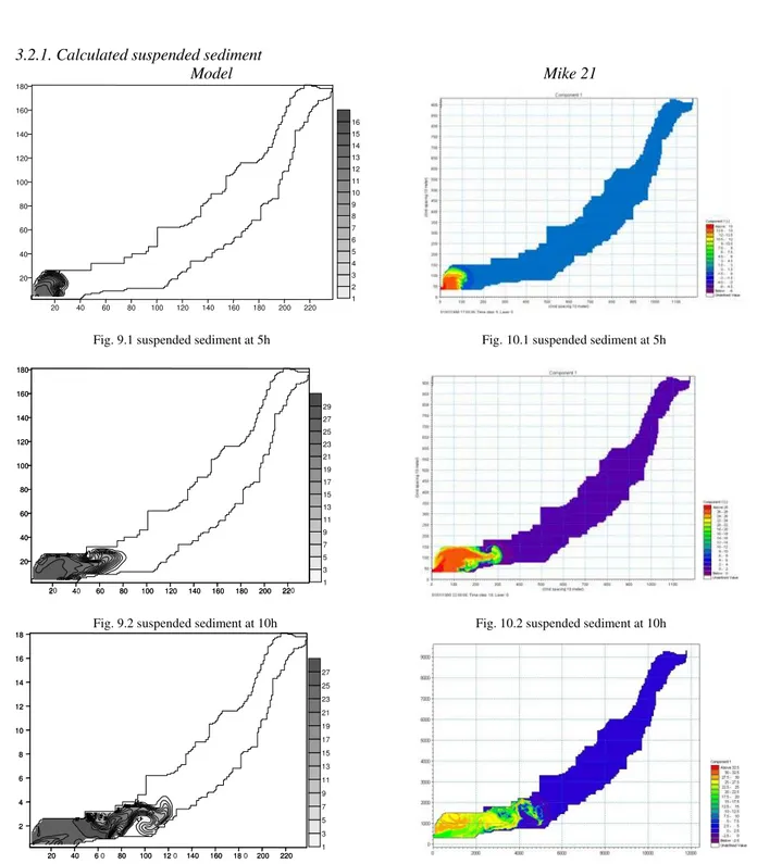
3.2.1. Calculated suspended sediment
Model Mike 21
Fig. 9.1 suspended sediment at 5h Fig. 10.1 suspended sediment at 5h
Fig. 9.2 suspended sediment at 10h Fig. 10.2 suspended sediment at 10h
Fig. 9.3 suspended sediment at 19h Fig. 10.3 suspended sediment at 19h
20 40 6 80 100 12 140 160 18 200 220
2 4 6 8 10 12 14 16 18
20 40 6 0 80 100 12 0 140 160 18 0 200 220
2 4 6 8 10 12 14 16 18
1 3 5 7 9 11 13 15 17 19 21 23 25 27
2 4 60 80 100 120 140 160 180 200 22
20 40 60 80 100 120 140 160 180
20 40 60 80 100 120 140 160 180 200 220
20 40 60 80 100 120 140 160 180
1 3 5 7 9 11 13 15 17 19 21 23 25 27 29
20 40 60 80 100 120 140 160 180 200 220
20 40 60 80 100 120 140 160 180
At 5h, concentration entering to the reservoir is 15g/l, flow velocity here is low, sediment suspension move slowly and decrease rapidly, 1400 m after reservoir inlet where concentrations are lower than 1g/l and velocities lower than 0.1m/s (Fig. 9.1 and Fig. 10.1).
In the upstream of the reservoir at maximum inflow at t=10h, sediments are convected due to important velocity inflow and concentrations increase until reaching maximum values of 29.08g/l at t=12hours as shown in fig.5b. Sediments move slowly towards the dam and concentrations decrease until less than 1g/l 4000 m after reservoir inlet, where velocities are about 0.3 m/s (Fig 9.2 and 10.2).
At t=19h, velocities decrease and convection too, sediment concentrations decrease progressively (Fig 9.3 and 10.3) and stop moving 6000 m after reservoir inlet where velocities are very low (0.01m/s).
Both models show nearly same concentration distribution in the reservoir. From figures 9 and 10, three main areas can be defined as follows:
At reservoir inlet, a delta can be formed where coarse materials can be deposited as velocity and transport capacity decrease. It depends of the geometry of the reservoir entrance. These results are similar to those given by [15] who investigated the influence of geometry of shallow reservoirs on flow patterns and sedimentation by suspended non cohesive sediment.
At upstream, high velocities with recirculation and therefore, high sediment transport are observed as for Stovin and Saul, 1994 [33] experiments results.
In Gargar reservoir, during this flood, suspended sediments move and progress in the reservoir with flow velocities, on a nearly distance of 8000m, without reaching the dam, but rather settle at the upstream of the reservoir. Sediment transport process is governed by the flow pattern [30] and [9].
4. Conclusion
Dam sedimentation induces storage capacity loss and therefore dam’s effective life.The main object of this study is to calculate the flow field in a dam reservoir with complex geometries, and to obtain qualitative knowledge of the suspended sediment transport, in order to predict deposit and transport areas during floods. The results of this study may be used to find out how to locate dam’s constitutive facilities and especially bottom control gates and equipments during the design, in order to assure a correct function and lifespan. Two dimensional horizontal model, elaborated from the resolution of the Saint Venant hydrodynamic system equations, using the Mac Cormack explicit finite difference scheme have been proposed, and coupled to the resolution of the “convection-diffusion” equation for a suspended non-cohesive particles, using the up-wind explicit scheme. A rectangular fully dense grid has been used to discretize the area.
Finally the developed model has been applied to a dam reservoir, in order to simulate flow field and sediments transport during flood.
The obtained results presented here, indicate that, according to the reservoir geometry and bathymetry, flow velocities increase when water depths diminish and sediment transport is due to water flow velocity, and low flow velocity is the reason of sediment particles deposit. Comparison between the obtained numerical model results and Mike 21, give generally a good satisfaction, and quite encouraging results. The proposed model may be able to simulate and predict flow field, such as water depth and horizontal components of depth-averaged velocity, and suspended sediment in a dam reservoir.
It has to be pointed out that the proposed model is still of preliminary and qualitative nature, more verifications, tests and some experimental work are still needed to demonstrate its performance and applicability.
Acknowledgement
All our thanks to the L.E.M (National laboratory of maritime studies) who permit us to use the Mike 21 license and (LEGHYD) Hydraulic Laboratory of Houari-Boumediene University.
References
[1] Brune, G. M., (1953): Trap efficiency of reservoir. American Geophysical Union. vol 34, num 3.
[2] Capolini, J.; Pieyns, S.; Ramana, R., (1969). Bassin versant du Cheliff. Etudes des caractères physiographiques et prévision des apports annuels, des crues et des transports solides dans les bassins du Rhiou, Sly, Fodda, Deurdeur, Zeddine, Ebda. Alger, Direc de l'Hydr.
[3] Chaudhry, M. H., (2008): Open-Channel Flow, 2e Ed, Springer Science.
[4] Cole, P.; Miles, G. V., (1983): A Two Dimensional Model of Mud Transport. ASCE J. Hyd. Jour of waterway, Port, Coastal and Ocean Engineering, ASCE, 111(6), pp 1041-1059.
[5] Dalmo, A. Vieira.; Weiming, Wu., (2002): One-Dimensional Channel Network Model CCHE1D Version 3.0, User's Manual. [6] Duan, J.G., (2004): Simulation of flow and mass dispersion in meandering channels. J. of Hydr Eng,
[7] Demmak, A., (1982): Contribution à l’étude de l’érosion et des transports solides en Algérie septentrionale. Thèse de doctorat, Paris [8] De Villiers, J.W., (2006): 2D Modeling of turbulent transport of cohesive sediments in shallow reservoirs. Thesis, Stellenbosch Univ [9] Dufresne, M.; Dewals, B. J.; Erpicum, S.; Archambeau, P.; Pirotton, M., (2010): Experimental investigation of flow pattern and
[10] Fiedler, F.R.; Ramirez, J.A., (2000): A numerical method for simulating discontinuous shallow flow over an infiltrating surface. J of Numerical Methods. Fluids. pp 219 – 240.
[11] Garcia, P.; Kahawita, R., (1986): Numerical solution of the Saint Venant equation with the Mac Cormack finite difference scheme. Internat J. for numerical methods in fluids, pp 259-274.
[12] Garg,V.; Jothiprakash,V., (2008): Estimation of useful life of a reservoir using sediment trap efficiency. J of Spatial Hydro, Vl8 No.2 [13] Graf, W. H.; Altinakar, M. S., (2000): Hydraulique fluviale, Ecoulement et phénomènes de transport dans les canaux à géométrie
simple, Ecole Polytechnique Fédérale de Lausanne.
[14] Ghenim, A.; Terfous, A. ; Seddini, A., (2007): Etude du transport solide en suspension dans les régions semi-arides méditerranéennes. Sécheresse V18, No 1
[15] Kantoush, S. A., (2008): Experimental study on the influence of the geometry of shallow reservoirs on flow patterns and sedimentation by suspended sediments. LCH, Lausanne.
[16] Kassoul, M.; Abdelkader, A.; Belorgey, M., (1997): Caractérisation de la sédimentation des barrages en Algérie, revue des sciences de l’eau, Paris – Québec.
[17] Lesser, G. R.; Roelvink, J. A.; Van Kester, J.A.T.M.; Stelling, G. S., ( 2004): Development and validation of a three-dimensional morphological model. J. Coastal Eng.
[18] Lu Yong-jun Zhang Hua-qing., (1993): Numerical simulation of degradation downstream of a reservoir. Model framework. J. of Hydrodynamics.
[19] Mattard, A., (1983): Modelisation numerique bidimentionnelles du transport de sediment fins. Maitrise de l’école polytech Montréal. [20] Nguyen, K. D.; Guillou, S.; Chauchat, J.; Barbry, N., (2009): A two-phase numerical model for suspended-sediment transport in
estuaries. Advances in Water Resources Elsevier.
[21] Nguyen, D. K.; Shi Yu-E.; Wang, S.Y.; Nguyen, Hung., (2006): 2D Shallow-Water Model Using Unstructured Finite-Volumes Methods. J. of Hydr Eng.
[22] Odd, N.V.M.; Owen, M.W., (1972): A two layer model of mud transport in Thames Estuary. Proc, Institution of Civil Eng, London. [23] Rahuel, J. L.; Holly, F. M.; Chollet, J. P.; Belleudy, P. J.; Yang, G., (1989): Modeling of River bed evolution for Bedload Sediment
Mixtures. J. Hydr Eng.
[24] Raju Ranga, K. G., (2009): Sedimentation of rivers, reservoirs and canals. Fresh surface water – Edited by James C.I.Dooge Vol III. [25] Randle, T.J.; Yang, C.T.; Daraio, J., (2006): Erosion and reservoir sedimentation. In Erosion and sedimentation manual. U.S.
Department of the Interior. Sedimentation and River Hydraulics Group. Denver, Colorado
[26] Remini, B., (1997) : Envasement des retenues de barrages en Algérie: Importance, mécanismes et moyens de lutte par la technique de soutirage. Thèse de doctorat d’état. Eco Polytech, Alger.
[27] Rijn, L. C., (1993): Principles of sediment transport in rivers, estuaries and coastal seas, Copyright, Aqua Publi. Delft Hydraulics. [28] Sabbagh-Yazdi, S. R.; Mastorakis, N. E.; Saeedifar; A.B., (2008): A cell center finite volume depth average flow solver for simulation
of erosion, transport and deposition of fine non-cohesive sediments. Int. J. of Computers. pp 47-57 [29] Saiedi, S., (1997): Coupled Modeling of Alluvial Flows. J. Hydraulic. Eng. Volume 123
[30] Saul, A. J.; Ellis, D. R., (1992): Sediment Deposition in Storage Tanks. Water Science & Technol Vo25 No 8 pp 189–198 © IWA Pub [31] Sheng, Y. P., (1983): Mathematical modeling of three dimensional coastal currents and sediment dispersion. Model development and
application, Technical Report CERC-83-2, Aeronautical Res Associates of Princeton, Inc., N.J.
[32] Simões, F. J.; Yang, C. T., (2006): Sedimentation modeling for rivers and reservoirs, in Yang, C.T., ed., Erosion and Sedimentation Manual. U.S. Bureau of Reclamation, Technical Service Center.
[33] Stovin Virginia, R.; Adrian, J. Saul., (1994): Sedimentation in Storage Tank Structures. Water Science & Technology. Vol 29 No 1-2 pp 363–372 © IWA Publishing
[34] Thiebot, J., (2008): Modelisation numerique des processsus gouvernant la formation et la degradation des massifs vaseux. Thèse de Doct de l’Ecole Génie Rural des Eaux et des Forêts. Paris
[35] Touaibia, B., (2010): Problématique de l’érosion et du transport solide en Algérie septentrionale. Sécheresse Vol 21.
[36] Wang, S. Y.; Wu, W., (2004): River sedimentation and morphology modelling-the state of the art and future development. Proceedings of the ninth international symposium on river sedimentation, Yichang, China.