A conceptual model for sheet-flow drawn from rapid granular flow

(1)

Rui M. L. Ferreira

1

_{, Vanessa A. Nicolau}

2

_{, S´ılvia R. Amaral}

3

_,

Jo˜ao G. A. B. Leal

4

_{& Ant´onio B. Almeida}

5

1

_{CEHIDRO-Instituto Superior T´ecnico, TULisbon, Av. Rovisco Pais, 1049-001}

Lisboa, Portugal, [email protected]

2

_{CEHIDRO-Instituto Superior T´ecnico, TULisbon, Av. Rovisco Pais, 1049-001}

Lisboa, Portugal, [email protected]

3

_{Laborat´orio Nacional de Engenharia Civil, Av. do Brasil, 101, 1700-066 Lisboa,}

Portugal, [email protected]

4

_{Dept. of Civil Engineering, Faculty of Sciences and Technology, UNL, Quinta}

da Torre, 2829-516 Caparica, Portugal; e-mail: [email protected]

5

_{CEHIDRO-Instituto Superior T´ecnico, TULisbon, Av. Rovisco Pais, 1049-001}

Lisboa, Portugal, [email protected]

ABSTRACT

This paper is aimed at presenting i) a simple, yet sound, conceptual model

ap-plicable to the simulation of erosion, deposition and transport of cohesionless

sediment in stratified flows under high shear stresses and ii) numerical solutions

in idealized unsteady flow non-equilibrium transport situations. The conceptual

model for the granular phase comprises 2DV mass and momentum and energy

equations and constitutive equations, all derived within the dense limit of the

Chapman-Enskog kinetic theory. 1D shallow-flow conservation and closure

equa-tions are derived for the fluid-granular mixture. Formulas for the average velocity

in the transport layers, the vertical net flux of sediment mass and the thickness of

the transport layer are thus obtained. Numerical solutions for dam-break flows

over cohesionless mobile beds in prismatic and non-prismatic channels are

ob-tained and discussed.

Keywords

: Granular flows, sheet-flow, dam-break

1 INTRODUCTION

This paper is consecrated to the development of a one-dimensional conceptual

model applicable to flows with high geomorphic potential, herein geomorphic

flows. A large number of flows can be included in this category, including rock

or snow avalanches, debris flows or river flows in the upper regime exhibiting

sheet flow. They have in common the ultimate driving mechanism, gravity, the

fact that they are slender flows and the fact that they occur at or generate high

shear stresses. Another common feature is the importance of the micromechanical

characteristics of the sediment in the definition of the constitutive equations.

Given the common features, the conceptual model will be developed for

sheet-flows, i.e. clearly stratified flows with a transport layer under high shear stresses,

but is expected to be applicable also to debris-type flows, i.e. flows of a dense

mixture of granular material and water whose transport layer occupies the full

flow depth.

(2)

smooth, round and only slightly inelastic the kinetic theory requires only small

modifications in order to provide 2DV conservation laws for the mass,

momen-tum and fluctuating energy of the granular material and constitutive equations

for the stress tensor, conductivity and viscosity coefficients and dissipation rate.

The inclusion of frictional effects and viscous fluid-grain interactions is done by

patching in

ad hoc

_{theories (Ferreira 2005, p. 249). The 2DV conceptual model}

is presented in Section 2. In the same section, the 2DV equations are

depth-averaged, in accordance with the shallow-flow hypothesis and with appropriate

kinematic boundary conditions. The continuum hypothesis is employed to merge

the necessary conservation equations expressing 1D mass and momentum

conser-vation.

In Section 3, the closure equations are obtained by process of numerical

exper-imentation. The 2DV conservation and constitutive equations of the transport

layer are solved in steady uniform conditions. Formulae for the average velocity

in the transport layers, the vertical net flux of sediment mass and the thickness

of the transport layer are obtained.

As they generate both sheet-flows and debris-like flows, dam-break flows are

adequate to test the solutions of the conceptual model. Numerical solutions

obtained for dam-break flows over cohesionless mobile beds, in prismatic and

non-prismatic channels, are presented in Section 4.

2 CONSERVATION EQUATIONS

Sheet-flow is a two-dimensional stratified flow involving a mixture of water and

granular material, picked up from the bottom. The granular phase is composed

of cohesionless sediment grains, nearly elastic, slightly rough and approximately

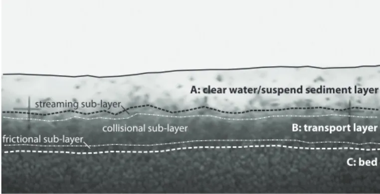
spherical. The fluid is viscous and incompressible. The flow structure is depicted

in Figure 1. Three main layers are promptly identified:

A

_{, characterized by small}

mean sediment concentrations or by clear water and where turbulent stresses are

dominant;

B

_{a transport layer, featuring decreasing concentrations upwards and}

stresses mainly originated in the granular phase and

C

_{the bed, composed of}

grains with no appreciable horizontal mean motion.

A: clear water/suspend sediment layer

B: transport layer

C: bed

frictional sub-layer

collisional sub-layer

streaming sub-layer

Figure 1. Detail of a sheet-flow with highlighted layered structure.

In layer

B

_{, it is expected that granular collisional stresses are dominant except}

in a thin bottom boundary layer where frictional stresses are dominant. The

collisional dominance assumption simplifies the expressions of the bulk granular

viscosity and of the granular conductivity (details in Ferreira 2005, pp. 231-250).

The 2DV conservation equations of layer

A

_{are the Reynolds-averaged}

Navier-Stokes equations. For layer

B

_{, the mass and momentum conservation equations,}

derived within the framework of the Chapman-Enskog theory, are, respectively

ρ

(g)

_D

t

(ν) +

ρ

(g)

νu

(i,ig)

= 0

(1)

ρ

(g)

νD

t

(3)

3 2ρ

(g)_ν_D

t(Θ) =−Φi,i+Tij(g)u (g)

j,i −γ(gw) (3)

whereρ(g) _{is the density of the sediment grains,}_nu _{is the solid fraction} (concen-tration at a specific point in the flow), u(_ig) is the velocity field of the granular phase,P(g) _{is the granular pressure,}_T(g)

ij is the granular stress tensor,f (gw)

j is the

force per unit volume expressing the interaction (essentially of viscous nature) of fluid and granular phases, Θ is the granular temperature, Φi is the flux of

fluctuating energy andγ(gw) _{is the rate of dissipation, due to inelastic collisions} and viscous damping (details in Ferreira 2005, pp. 247-249), of the fluctuat-ing energy. In equations (1) to (3) the operator Dt(·) stands for the material

derivative for which the convective operator is relative to the mean low, Ein-stein’s notation is used for space derivatives and the bracket operator · stands for point-wise time or ensemble average (ergodicity is assumed). Equation (3) reveals that, unlike thermodynamic systems a granular system can maintain a steady state of agitation, characterized by a given granular temperature, if and only if the rate of production equals the diffusive flux and the dissipation, i.e. if

T_ij(g)u_j,i(g) = Φi,i+γ(gw).

Conservation equations are also needed for the water phase. These can be obtained from a control volume analysis within the continuum hypotheses:

−ρ(w)Dt(ν) + (1−ν)ρ(w)u(i,iw)= 0 (4)

(1−ν)ρ(w)_D t

u(_jw)=−P_,j(w)+T_ji,i(w)+ (1−ν)ρ(w)_g

j−fj(gw) (5)

where ρ(w) _{is the density of the fluid,} _u(w)

i,i is the fluid velocity field, P(w) is the

isotropic fluid pressure, T_ij(w) is the fluid stress tensor.

In order to derive the 1D conservation equations, i) the 2DV equations of conservation of each constituent are summed (equations 1 and 4 and 2 and 5), ii) cinematic boundary conditions are applied the free-surface, bed and margins and iii) the equations are depth-integrated, within the continuum hypothesis. The 1D conservation of total mass is

∂tA+∂x(uh) =−∂tA0=−

_Q

b−Q∗ b

(1−pb)Λ−Al

(6)

whereA=Aw+Ab,Ab= hb

0 σ(η)dηis the area of the cross-section occupied by layer B_, _h_b _{is the thickness of layer} B_, _A_w _{is the area corresponding to layer} A_,

A0 is the area below the channel (the channel bed), Qb = CbubAb is the actual

volumetric sediment discharge, Cb is the actual sediment concentration, Q∗b =

C∗

bubAb is the equilibrium sediment discharge, Cb∗ is the equilibrium sediment

concentration, ub is the velocity of B, pb is bed porosity, Λ is an adaptation

length (the length scale of non-equilibrium sediment transport) and Al is the

lateral contribution of mass from the channel banks. In the proposed model, the calculation ofAl is simplified, as shown in Figure 2.

∆Zb

A

Erosion. No failure

l

∆Zb

Erosion. Bank failure

A_l

∆Zb

Deposition

(4)

The equation of conservation of total momentum is

∂tM +∂x

ρbu2bAb+ρ(w)uw2Aw+ρbgIb+ρ(w)gIw

+g

ρbAb+ρ(w)Aw

∂xZb=−τbP+gρbKb+gρ(w)Kw (7)

where Zb is the bed elevation, M = ρbAuis the mass discharge, u is the

layer-averaged velocity,uw is the velocity of layerA,τbis the bed shear stress,P is the

wetted perimeter,ρb=ρ(w)(1 + (s−1)Cb), s=ρ(g)/ρ(w) andIb, Iw,Kb and Kw

are impulsion terms.

The equation of conservation of mass in the transport layer is

∂tHb+∂x(Hbub) =−

_Q

b−Q∗ b

Λ −T(1−pb)

(8) where the conservative variable isHb=AbCb.

The equation of conservation of the bed is (1−pb)∂tA0= Qb−Q

∗ b

Λ −Al(1−pb) (9)

The system of equations (6), (7), (8) and (9) admits four unknowns, the conservative variablesA,M,HbandA0. At each time step, the primitive variables

u,Cbmust be computed from the conservative ones.

Closure equations for hb, ub, τb, Cb∗ and Λ are needed. They will be derived

in the next section within the same granular dynamics paradigm.

3 CLOSURE EQUATIONS

Numerical experiments are performed to derive the closure equations. A detailed characterization of the two-dimensional (vertical) flow in the transport layer is obtained by solving numerically the following set of ODEs

dY

dz =M(Y, z) (10)

whereY=

T(g) _P(g) _u(g)

x Θ Φ ν T(w) P(w) u(xw) T

and

M(Y, z) =

                  

−ρ(g)_νg_sin(_β₎₋_f D

−ρ(w)₍_s₋₁₎_νg 5π1/2

8

T(g) νρ(g)_ϑ₁_ϑ₃_d_s_Θ11/2

−π1/2 4

1 νρ(g)_ϑ

1ϑ4 Φ dsΘ1/2

5π1/2 8

(T(g)₎2

νρ(g)_ϑ₁_ϑ₃_d_Θ11/2 −_π241/2

1−e(gw)

ρ(g)_νϑ 1Θ

3/2 d π1/2

4

1+ϑ1

ρ(g)_ϑ 1ϑ4

1+8ϑ1+4ν2dg0 dν

Φ

dΘ3/2− s−_s1

gν

1+8ϑ1+4ν2dg0 dν

Θ

−ρ(w)₍₁₋_ν₎_g_sin(_β_{) +}_f D

−ρ(w)_g

T(w) ρ(w)

1/2 1 κz(1−ν)1/2f(ν)

                   (11)

(5)

0 2 4 6 8 10 12 14 16

-5 -4 -3 -2 -1 0 1 2 3 4 5

dissipation, diffusion and production

z

/

d

3 21

1 2 3 3 2 1

0 2 4 6 8 10 12 14 16

0 5 10 15

velocity z / d 1 2 3 0 2 4 6 8 10 12 14 16

0 0.2 0.4 0.6

solid fraction

z

/

d ₁2

3 0 2 4 6 8 10 12 14 16

0 0.5 1 1.5 2

granular temperature z / d 1 2 3 0 2 4 6 8 10 12 14 16

-8 -3 2

flux

z

/

d

3 2 1

0 2 4 6 8 10 12 14 16

0 1 2 3 4

granular shear stress

z / d 3 2 1

(a) (b) (c)

(d) (e) (f)

u( )g_/_Ög s₍_-₁₎d

s

¾¾¾¾ _n _Q_{/ (}₍_{g s}_-₁₎_d₎

s

T( )g_/_(r g s₍_-₁₎d₎

s ( )w

F/(r (( )w _{g s}₍-₁₎_d) )

s3/2

non/dimentional dissipation, diffusion and production

z d / z d / z d / z d / z d / z d /

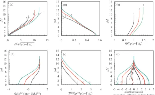
Figure 3.

Computed profiles of non-dimensional quantities in the

transport layer. Simulations 1, 2 and 3 correspond to, respectively,

θ

= 1.74

,

θ

= 2.49

and

θ

= 3.07

.

(details in Ferreira 2005, pp. 252-256). The results for plastic pellets with

d

=

0.003 m,

s

= 1.27 and coefficient of restitution

e

= 0.825 are shown in Figure 3.

Equations for

h

b

,

u

b

,

τ

b

and

φ

nets3,2

= (Q

b

−

Q

∗b

)/Λ follow from the solution

shown in Figure 3. The existence of a frictional layer across which the shear

stress may vary allows for determining the mass flux between the bed and the

transport layer. The integration of the equation of conservation of momentum in

the vertical direction over the frictional layer renders (Ferreira (2005) p. 279)

∂

t

(A

0

b

−

Q

∗b

)

(12)

where

Z

f

is the elevation of boundary between the frictional and collisional layers.

In equation (12) it is implicit that the equilibrium concentration is

C

∗

(13)

and the adaptation length is

Λ =

u

b

(ρ

b

u

x

)

|

z=Zf

gρ

(w)

_(s

₋

_{1) (1}

₋

_p

b

) tan (ϕ

b

)

(14)

As seen in Figures 3c and 3d, the the modulus of the flux of the fluctuating

kinetic energy increases toward the bed and the granular temperature is never

zero. This means that fluctuating energy is constantly being extracted from the

mean flow and directed toward the bottom. As a consequence, the frictional

sub-layer cannot increase indefinitely. It is assumed that this sub-layer has a thickness of

2d. The value of the concentration in

ρ

b

and of (u

x

)

z=Zf

can be read in Figures

3b and 3a, respectively. An estimate for the velocity in the transport layer can

be obtained by fitting the profiles of Figure 3a:

u(z)/u

=

11₆

(z/h)

5/6

(15)

where

h

is the flow depth. The depth-averaged velocity becomes

(6)

Depth-averaging the equation of conservation of the fluctuating energy,

Fer-reira (2005), pp. 278-287, obtained and algebraic relation for the thickness of

the transport layer. Taking in account the values of the restitution coefficient

and the internal friction angle at the bed, the non-dimensional thickness of the

transport load layer appears to depend little on the type of sediment and may be

approximated by

h

b

/d

= 1.7 + 5.5θ

(17)

In rivers undergoing sheet-flow, flow resistance is only marginally influenced

by the particular shape of the stream bed, as alluvial bed forms are absent. The

micromechanical properties of the sediment and the interaction with the fluid, in

particular the energy dissipation in binary collisions and the interstitial viscous

dissipation, are the mechanisms to accommodate in the characterization of the

flow resistance. The results of Sumer et al. (1996) allow for the computation

of the friction factor. It was found that the bed shear stress can be adequately

described by

τ

b

≡

is the fall velocity is considered

to be 2.

4 COMPUTATIONAL RESULTS

The important formative potential of dam-break flows implies that they transport

an extremely high sediment load over long distances. They generally feature

debris-like characteristics at the wave front and a stratified sheet-like flow behind

it. The overall quality of the model is thus tested in dam-break flows performed

in idealized conditions, namely, instantaneous rupture and cohesionless mobile

bed. Mathematically, it is a Riemann problem, a particular Cauchy problem.

Written in vector notation, the first order, non-homogeneous, hyperbolic

sys-tem of conservation laws (equations 6, 7 and 8) that describe geomorphic

dam-break flows is

∂

t

(

V

(

U

)) +

∂

x

(

F

(

U

)) =

G

(

U

)

(19)

where

V

:

Ê

x

]0,

+

∞

_{is the vector of the source terms and}

_x

_and

_t

_{are the space and}

time co-ordinates, respectively.

A validation test was performed by comparing the results of the model with

laboratory results performed at UCL, Louvain-la-Neuve, Belgium (details in Benoit

2005 pp. 56-56 and Ferreira et al. 2006). The sediment particles were PVC

pel-lets with

s

= 1.56 kg m

−3

_{and equivalent diameter}

_d

_{= 3.9 mm. The dimensions}

of the particles exhibited little variability. The initial conditions, in terms of

h

L

, the upstream water depth,

Z

bL

, the upstream bed elevation,

h

R

, the

down-stream water depth,

Y

L

the upstream elevation above the upstream bed level,

α

≡

hR+

|

min

)

, are shown in Table 1.

Table 1. Summary of the initial data for experimental tests.

h_L Y_b

L hR YL α δ

Name

(m) (m) (m) (m) (−) (−) 35 00 00 0.₃₅ ₀.₀₀ ₀.₀₀ ₀.₃₅ ₀.₀₀₀ ₀.₀₀₀

35 10 00 0.₂₅ ₀.₁₀ ₀.₀₀ ₀.₃₅ ₀.₀₀₀ ₀.₂₈₆

35 10 10 0.₂₅ ₀.₁₀ ₀.₁₀ ₀.₃₅ ₀.₂₈₆ ₀.₂₈₆

(7)

found, especially for the flat bed case (test 35 00 00). Tests 35 10 00 and 35 10 10

show two different types of hydraulic jump that may occur in the

α

−

δ

plane

(Ferreira 2005, Ferreira et al. 2006). Due to the low downstream water depth in

test 35 10 00, the jump is induced by the non-equilibrium transport and friction

(Capart & Young 1998). The the jump observed in 35 10 10 is independent of the

source terms in equation (19). A general poor agreement in the bed elevation is

found in the vicinity of the gate, due to un-acountable geotechnical slope failure.

Figure 4. Computed and measured of the flow profiles corresponding

to the tests identified in Table 1

In order to test the effects of the variability of channel configuration and the

influence, on the final solution of the parameters that govern lateral bank failure,

a test was performed with trapezoidal erodible banks. Initial conditions comprise:

Z

bL

= 0.06 m,

h

L

= 0.21 m and

h

R

= 0.0 m. The initial bed width is

b

f

= 0.15

m and the inverse bank slopes are

m

= 0.84, which corresponds to an initial

bank slope angle of 50

o

_{. This channel configuration mimics the experimental}

tests presented by Le Grelle et al. (2003). The material of the bed and margins

is sand with

d

= 1.8 mm,

s

= 2.62, tan(ϕ

b

) = 0.4. For the sake of numerical

stability, the friction coefficient was

C

f

= 0.0067.

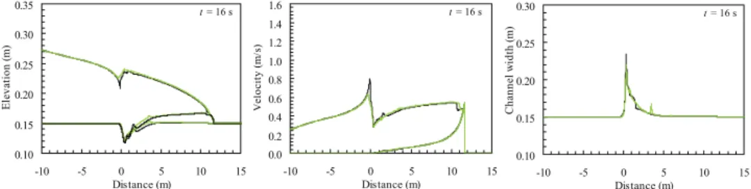
Numerical results are obtained with a conservative firs order flux difference

splitting discretization based on Euler’s method and Roe’s Riemann solvers

(de-tails in Ferreira 2005, pp. 465-479). The results are shown in Figure (5). Two

scenarios are shown, SimBe1 for which the critical bank slope is

m

cr

= 0.7 and

SimBe2 for which

m

cr

= 0.825. The equilibrium bank slope was, in both cases

m

eq

= 0.839.

0.10 0.15 0.20 0.25 0.30

-10 -5 0 5 10 15 Distance (m)

C

h

a

n

e

l

w

id

th

(

m

)

t = 16 s

0.0 0.2 0.4 0.6 0.8 1.0 1.2 1.4 1.6

-10 -5 0 5 10 15 Distance (m)

V

e

lo

c

it

y

(

m

/s

)

t = 16 s

0.10 0.15 0.20 0.25 0.30 0.35

-10 -5 0 5 10 15 Distance (m)

E

le

v

a

ti

o

n

(

m

)

t = 16 s

Figure 5. Longitudinal profiles of the flow depth, bed elevation and

thickness of the transport layer (left), layer-averaged velocity and

ve-locity in the transport layer (center) and channel width at the initial

bed elevation (right).

X

′

_{= (x/t)/}

√

_gY

The conceptual model presented in this paper is applicable to geomorphic

strati-fied flows featuring sediment transport at high shear stresses. The dense limit of

Chapman-Enskog’s kinetic theory is at the root of the 1D closure equations. This

means that the interaction between sediment and fluid phenomena is conceived

to occur, fundamentally, at the grain-scale.

The model was tested for internal consistency and compared with

experi-mental evidence. Dam-break flows were chosen as applications, for its ability to

generate stratified flows with high shear stresses. The computational results

sug-gest that the model assumptions, namely the emphasis on grain-scale phenomena

as the most relevant for developing closure models, may be valid for a wider range

of actual geomorphic flows.

ACKNOWLEDGMENTS

This research as partially supported by the project PIRE0730246 “Modeling

of Flood Hazards and Geomorphic Impacts of Levee Breach and Dam Failure”

funded by the US National Science Foundation.

REFERENCES

Armanini, A.; Capart, H.; Fraccarollo, L.; Larcher M. (2005) Rheological

stratification in experimental free-surface flows of granular-liquid mixtures.

J. Fluid Mech.532

_{:269-319 .}

Capart, H. & Young, D.L. (1998) Formation of a jump by the dam-break

wave over a granular bed.

J. Fluid Mech.372

_:165-187.

Chapman, S. & Cowling, T. G. (1970).

The Mathematical Theory of Non-Uniform Gases,

3rd Ed. Cambridge University Press.

Lun, K. K.; Savage, S. B.; Jeffery, D. J. & Chepurny, N. (1984) Kinetic

theories for granular flows: inelastic particles in Couette flow and slightly

inelastic particles in a general flow field.

J. Fluid Mech.140

_{: 223-256.}

Ferreira, R. M. L., (2005)

River Morphodynamics and Sediment Transport. Conceptual Model and Solutions.

PhD Thesis, Instituto Superior T´ecnico, TU

Lisbon.

Ferreira, R.M.L.; Amaral, S.; Leal, J.G.A.B. & Spinewine, B., (2006),

Dis-continuities in geomorphic dam-break flows.

River Flow 2006

, Vol. 1: 1521-1530,

Balkema. ISBN0415408156.

le Grelle, N., Soares Fraz˜ao, S., Spinewine B. & Zech Y. (2003).

Dam-break flow experiment: Geomorphic changes in a valley with uniform

sedi-ment. Proc. 3rd IMPACT Workshop, UCL Louvain-la-Neuve, 5-7 November.

Jenkins, J. T. & Richman, M. W. (1988) Plane simple shear of smooth

inelastic circular disks: the anisotropy of the second moment in the dilute and

dense limits.

J. Fluid Mech.192

_:313-328.

Spinewine, B. (2005)

Two-layer flow behavior and the effects of granular dilatancy in dambreak induced sheet-flow.